Systematic Study of Gravitational Waves from Galaxy Merger

Abstract

A systematic study of gravitational waves from galaxy mergers, through $N$-body simulations, was performed. In particular, we investigated the relative importance of galaxy components (disk, bulge and halo) and effects of initial relative velocity, relative angular momentum and mass ratio of the galaxies. We found that the features of light curve of gravitational waves, such as peak width and luminosity, are reliably simulated with particle numbers larger than $\sim 10^{4}$. Dominant contribution to gravitational wave emission came from the halo component, while peak luminosity amounted to $10^{31}~{}{\rm erg/sec}$ for the collision of two halos with mass $3.8\times 10^{12}h^{-1}M_{\odot}$. We also found that the initial relative velocity in the direction of the initial separation did not significantly affect gravitational wave emission, while the initial relative angular momentum broadened the peak width and suppressed the luminosity. Mass dependence of the peak luminosity was also investigated, and we obtained evidence that the luminosity is proportional to the cubic mass when the scaling relation is satisfied. This behavior was considered by a simple analysis.

I Introduction

Structure formation of the universe proceeds through gravitational interaction from tiny density fluctuations. In this process, gravitational waves with cosmological scales are expected to be produced. In Mollerach et al. (2004); Ananda et al. (2007); Baumann et al. (2007), generation of gravitational waves was studied as a second-order effect of cosmological perturbations. It was shown that the density of gravitational wave background, $\rho_{\rm GW}$, amounts to $\rho_{\rm GW}/\rho_{\rm c}\sim 10^{-20}-10^{-15}$ for a wide frequency range, where $\rho_{\rm c}$ is the critical density. At smaller scales, gravitational waves, radiated through the formation of dark matter halo, were studied in Carbone et al. (2006) and the density was estimated as $\rho_{\rm GW}/\rho_{\rm c}\sim 10^{-20}$ at frequencies $10^{-18}-10^{-17}~{}{\rm Hz}$. Thus, these processes of structure formation are imprinted on the gravitational wave background.

Although such gravitational wave background of cosmological scales is inaccessible to direct detection, it could be probed by measuring the B-mode polarization of the cosmic microwave background. In actuality, several missions suited for this aim have been planned; for example, LiteBIRD, QUIET, POLARBeaR (see, http://cmbpol.kek.jp/index-e.html), and Cosmic Inflation Probe (see, http://www.cfa.harvard.edu/cip/). Their primary purpose is to detect primordial gravitational waves generated during inflation. However, it was reported in Carbone et al. (2006) that gravitational waves from halo formation could be dominant if the energy scale of inflation is below $\sim 10^{15}~{}{\rm GeV}$.

In this paper, we investigate galaxy merger as another process which produces gravitational waves of cosmological scales. In the hierarchical model of structure formation, it is argued that low-mass dark matter halos repeatedly merge with each other to form more massive halos (see, e.g., Lacey and Cole (1993, 1994)). Because halo merger is a highly nonlinear process which involves huge masses, it is expected that substantial amounts of gravitational waves are emitted. In Quilis et al. (2007), gravitational waves from galaxy merger are calculated with $N$-body simulations. These researchers studied several typical configurations of galaxy merger and estimated the luminosity to be of order $10^{33}~{}{\rm erg~{}sec^{-1}}$.

By extending this previous study Quilis et al. (2007), we perform a systematic study of gravitational waves from galaxy mergers through $N$-body simulations with Gadget2 Springel et al. (2001); Springel (2005). While in Quilis et al. (2007) initial condition was generated by an open code “GalactICS” Kuijken and Dubinski (1995) and Jaffe model Jaffe (1983), here we use a halo adopted from a cosmological simulation as well as ones generated by “GalactICS”. The former has a realistic density structure which is well approximated by the Navarro-Frenk-White (NFW) profile Navarro et al. (1996). On the other hand, the latter describe disk galaxies with three components, disk, bulge and halo. With these initial conditions, we investigate the relative importance of galaxy components (disk, bulge and halo) and the effects of initial velocity, relative angular momentum and mass ratio of the halos. Also we check the dependence of the results on simulation resolution by varying the particle number. This study can be regarded as the first step toward evaluating the gravitational wave background from galaxy merger.

The paper is organized as follows. In section II, we explain our method of calculation, including the preparation of the initial conditions. In section III, the results are presented. Finally section IV is devoted to the summary of our study and discussion including our future plans.

II Method

We follow the merging process of two galaxies using the parallel $N$-body solver Gadget2 Springel et al. (2001); Springel (2005) in its Tree-PM mode. The gravitational softening parameter is set to around $1/60$ of the tidal radius of galaxies. We use two types of initial conditions (type A and B). Type A is prepared by generating galaxies with “GalactICS” while a realistic halo is adopted from a cosmological simulation for type B. Detailed description of the initial condition will be given in the next section.

Based on the $N$-body simulation, we compute the amplitude and luminosity of the gravitational waves. Here, we neglect the effect of cosmological expansion because the initial separation of galaxies is taken to be $\sim 1~{}h^{-1}{\rm Mpc}$ and the ratio of acceleration due to cosmic expansion and gravitational force between galaxies is of order $0.1$. Further, the velocity dispersion of stars in each galaxy and the relative velocity between two galaxies are nonrelativistic ($v/c\leq 10^{-3}$) so that the slow-motion approximation is valid. By denoting the deviation of the metric from Minkowski spacetime as $h_{\mu\nu}$, and taking the transverse-traceless (TT) gauge, the spatial components of $h_{\mu\nu}^{TT}$ are given by the quadrupole formula as

$$h_{ij}^{TT}=\frac{2G}{c^{4}r}\ddot{I}_{ij}(t-r/c),$$ (1)

where $G$ is the gravitational constant and $r$ is the distance from the observer to the merging galaxies. Here $I_{ij}$ is the components of the traceless internal tensor given by

$$I_{ij}=\sum_{k}m^{(k)}\left(x_{i}^{(k)}x_{j}^{(k)}-\frac{1}{3}\delta_{ij}{x^{(k)}}^{2}\right)$$ (2)

where $x_{i}^{(k)}$ represents the position of $k$-th particle. Later we will set the initial separation of two galaxies in the direction of $x$.

The luminosity of gravitational waves is given by

$$L_{\rm GW}=\left(\frac{dE}{dt}\right)_{\rm GW}=\frac{G}{5c^{5}}\sum_{ij}\dddot{I}_{ij}\dddot{I}_{ij}~{}~{}~{}{\rm[erg~{}s^{-1}]}.$$ (3)

It should be noted here that this formula needs third-order time derivatives which may cause a substantial numerical error. We will estimate the numerical error by three different calculational procedures in section III.1.

III Results

In this section, we present the results of our numerical simulations. In subsection III.1 we generate initial conditions using “GalactICS” and investigate the relative importance of the galaxy components (halo, disk and bulge). Also we check the convergency of the results by varying the particle number. In subsection III.2, we use initial conditions adopting a dark halo from a cosmological simulation. Finally we study the effects of the initial relative velocity, relative angular momentum and mass (ratio).

III.1 Simulations with Type A Initial Conditions

Table 1: Models used in this subsection. Column(1):model name. Column(2):total mass. Column(3):mass of halo. Column(4):mass of disk. Column(5):mass of bulge. Column(6):disk scale radius. Column(7):tidal radius.

model	$M_{\rm tot}~{}(10^{10}~{}M_{\odot})$	$M_{\rm h}$	$M_{\rm d}$	$M_{\rm b}$	$r_{\rm d}~{}({\rm kpc})$	$r_{\rm t}~{}({\rm kpc})$
model-0	31.1	26.5	3.9	0.7	4.5	56.5
model-A	31.9	25.0	4.4	2.2	4.5	98.9
model-D	195.6	188.9	4.5	2.2	4.5	330.7

First, let us describe the initial conditions. In this subsection III.1 we use initial conditions generated by “GalactICS” Kuijken and Dubinski (1995). This is based on a semi-analytic model for the phase-space distribution function of an axisymmetric disk galaxy, and outputs the distribution functions of a disc, bulge and halo from input parameters such as total mass and angular momentum. One of the advantages of using “GalactICS” is that it can create a disk galaxy with halo, disk and bulge of arbitrary mass self-consistently. We will see that the dominant contribution to gravitational wave emission comes from the halo component. Another advantage is that we can choose the number of particles arbitrarily so that we can study the effect of resolution on gravitational wave emission.

We prepared three initial conditions whose parameters are shown in TABLE 1. Here $r_{\rm d}$ and $r_{\rm t}$ are the scale radius of the disk and the tidal radius, which is the outermost radius of the halo Kuijken and Dubinski (1995), respectively. The model-0 is similar to the disk galaxy adopted in Quilis et al. (2007). As we can see in Fig. 1, the rotation curve is decreasing outward within $30~{}{\rm kpc}$, which means that the halo component is relatively concentrated. In this sense, this model is not so realistic. To study the effect of concentration on gravitational-wave emission, we consider model-A, which has almost the same mass as model-0 but a flatter rotation curve (Fig. 1). Further, model-D is considered to show the effect of mass and halo extension. Model-D has a similar mass and structure as our galaxy and the central density profile is similar to model-A. It should be noted that model-A and model-D are identical to model A and model D in Kuijken and Dubinski (1995). In this subsection, we will mainly use model-0 and, at the end, make a comparison between model-0 and model-A.

The particle number per galaxy is set to $5.4\times 10^{5}$ for all models in this section. Then we simulate the head-on merger of two identical galaxies with initial relative velocity in the $x$-direction which corresponds to the kinetic energy equal to potential energy.

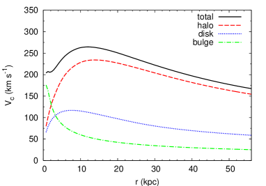
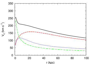
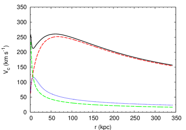
Figure 1: Rotation curve , $V_{c}(r)=\sqrt{GM(r)/r}$, for halo+disk+bulge (solid), halo (dashed), disk (dotted), and bulge (dash-dotted) for a range from galactic center to $r_{\rm t}$. Top: model-0. Middle: model-A. Bottom: model-D.

Figure 2: Time evolution of luminosity of gravitational waves for model-0.

Fig. 2 shows the time evolution of the luminosity of gravitational wave for model-0. We can see two major peaks which correspond to the collisions of two galaxies. These gradually relax into a single galaxy and gravitational-wave emission becomes much less effective after $t=1.2~{}{\rm Gyr}$. The peak width, $\sim 0.1~{}{\rm Gyr}$, reflects the dynamical timescale of the galaxies. The peak luminosity reaches $1.4\times 10^{30}~{}{\rm erg/sec}$ and the total emitted energy is about $\sim 10^{46}~{}{\rm erg}$. As we will see below, the steady emission after $t=1.2~{}{\rm Gyr}$ is substantially affected by the simulation resolution and would be considered as noise within the simulation. Therefore, there is a possibility that more peaks do exist below this noise level. Nevertheless, it is robust that the luminosities of the third and later peaks are less than $\sim 10^{26}~{}{\rm erg/sec}$ and make negligible contributions to the total luminosity.

As we saw in Eq. (3), we need the third-order derivatives of $I_{ij}$ to calculate gravitational wave luminosity. However, if we calculate these by differentiating $I_{ij}$ three times numerically, it may cause a substantial numerical error. Because Gadget2 outputs $\ddot{x}_{i}$ as well as $x_{i}$ and $\dot{x}_{i}$, it is possible to obtain $\dddot{I}_{ij}$ with just one numerical differentiation, allowing for the reduction of numerical error. To aide in estimating the error concerning the numerical differentiation, we show in Fig. 3 the comparison of gravitational wave luminosities calculated with three different approaches. F1 is calculated from $I_{ij}$ obtained by $x_{i}$, F2 is calculated from $\dot{I}_{ij}$ obtained by $x_{i}$ and $\dot{x}_{i}$, and, finally F3 is calculated from $\ddot{I}_{ij}$ obtained by $x_{i}$, $\dot{x}_{i}$ and $\ddot{x}_{i}$. We can see that the differences are smaller than factor 2 during almost the entire process. Thus, we can conclud that the error concerning the numerical differentiation is not a significant factor in our calculation. Hereafter, we adopt F3, which is expected to cause the least error among the three methods.

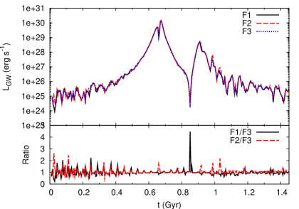
Figure 3: Top: comparison of gravitational wave luminosities calculated with three different approaches for model-0. See text for detail. Bottom: ratios of luminosity, F1/F3 and F2/F3.

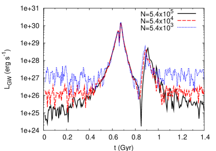
Figure 4: Dependence on particle number ($5.4\times 10^{5}$: solid, $5.4\times 10^{4}$: dashed, $5.4\times 10^{3}$: dotted). Other parameters are the same as the model-0.

Next, we compare the luminosity evolution by varying the particle number $N$ in Fig. 4. As can be seen, however, the two peaks are almost independent of the input particle number, while the steady emission after and before collision shows substantial increases for smaller $N$. Thus, we can expect that the feature of the peaks and total emitted energy can be studied reliably with particle numbers larger than $\sim 10^{4}$. This particle number should be compared with that of the simulations in the next subsection, $N=2.4\times 10^{5}$. On the other hand, the steady emission is affected by the resolution of simulation and would be highly suppressed in real galaxy merger.

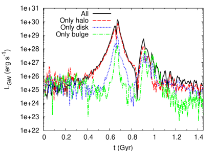
Figure 5: Time evolution of luminosity of gravitational waves for model-0 with contribution from halo (dashed), disk (dotted), bulge (dash-dotted) only. Total luminosity is also shown (solid).

Having established the above two elements of this model, we next study the relative importance of galaxy components. Although the mass of a galaxy is mostly due to the contribution from its halo, disk and bulge may also considerably contribute to gravitational wave emission because they are more concentrated than the halo itself. To account for this, we calculate the quadrupole $I_{ij}$, Eq. (2), for each component. However, the dynamics of particles in all components was solved taking the gravitational potential of all the particles into account. Fig. 5 shows the contribution of each component (halo, disk and bulge). We can see that, at the peaks, the luminosity is dominated by the contribution from the halo and other contributions are at most $12\%$. Remembering that the mass of the disk is about one seventh of that of the halo itself, and that the luminosity is apparently proportional to the squared mass. The contribution of the disk ($\sim 10\%$) is larger than a naive expectation. This would be due to the fact that the disk is more concentrated than the halo, so that the disk emits gravitational waves more effectively. We tested the effect of concentration of the disk component by changing the mass profile artificially. As a result, a disk with size $80\%$ and $120\%$ of the fiducial size contributes $14\%$ and $9\%$ of the total luminosity, respectively, while it is $12\%$ for the fiducial mass profile. Thus, it is expected that the gravitational wave luminosity is dominated by the halo component for a reasonable range of the disk concentration.

Furthermore, we note that the ratio of the luminous mass to the dark mass $M_{\rm dark}/M_{\rm lum}$ that we adopted is about 7, which is smaller than that of typical galaxies ($\sim 10$). Thus, our calculations are overestimating the disk and bulge contributions. This fact justifies our later calculations with galaxies obtained from a cosmological simulation which have only halo components.

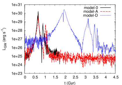
Figure 6: Time evolution of luminosity of gravitational waves for model-0 (solid), model-A (dashed), and model-D (datted).

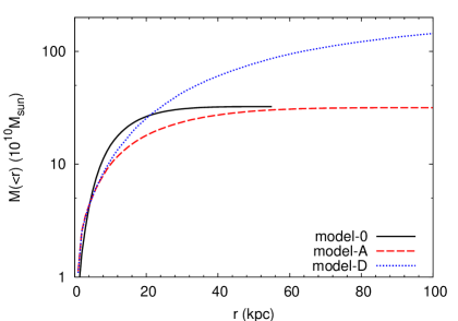
Figure 7: Top: the density profile of model-0 (solid), model-A (dashed), and model-D (dotted). Bottom: the mass of model-0 (solid), model-A (dashed), and model-D (dotted) within the radius.

Finally, we compare the gravitational-wave luminosities for mergers of model-0, model-A and model-D galaxies. The peak luminosity for model-A is $4.7\times 10^{29}~{}{\rm erg/sec}$, which is about one third of that of model-0, even though both models have almost the same mass. This is because model-0 has a more concentrated halo than model-A as can be seen from Fig. 7. On the other hand, the peak luminosity for model-D is $2.4\times 10^{30}~{}{\rm erg/sec}$, which is approximately 5 times larger than that of model-A. Since the bulge and disk components of model-A and D are almost identical, the difference of peak luminosities comes from the halo mass components of these models. The halo mass distributions of the two models are similar within 10 kpc, while model-D has more extended halo than model-A as is shown in the bottom panel of Fig. 10. Accordingly, the ratio of halo masses of model-D and A is about 7.6. Thus, gravitational-wave luminosity is very sensitive to both the mass and the density structure of halo, making quite clear the importance of using a realistic model. In the next subsection, we simulate mergers of galaxies with a NFW-like density profile and study the mass dependence.

III.2 Simulations with Type B Initial Conditions

Table 2: Models used in this subsection. Column(1):model name. Column(2):mass of one galaxy. Column(3):initial relative velocity (relative velocity in the $z$-direction is set to zero). Column(4):initial separation between the galaxies in the $x$-direction (initial separations in the $y$- and $z$-directions are set to zero).

model	$M(h^{-1}M_{\odot})$	$(\Delta V_{x},\Delta V_{y})$ (${\rm km~{}s^{-1}}$)	$\Delta x$ ($h^{-1}{\rm kpc}$)
A-1	$3.8\times 10^{12}$	(0,0)	1200
A-2	$3.8\times 10^{12}$	(220,0)	1200
A-3	$3.8\times 10^{12}$	(380,0)	1800
B-1	$3.8\times 10^{12}$	(0,0)	850
B-2	$3.8\times 10^{12}$	(0,70)	850
B-3	$3.8\times 10^{12}$	(0,140)	850
C-1	$3.8\times 10^{11}$	(0,0)	680
C-2	$3.8\times 10^{10}$	(0,0)	680

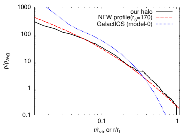
Figure 8: Top: Density profile of the fiducial halo with $1.3\times 10^{14}h^{-1}M_{\odot}$ (solid) which is well fitted by the NFW profile with $r_{\rm s}\sim 170~{}h^{-1}{\rm kpc}$ (dashed). For reference, the density profile of the galaxy (model-0) used in section III.1 is also shown (dotted). The density and the radius are normalized with the average density $\rho_{\rm avg}$, and the virial radius $r_{\rm vir}$ of each galaxy. However, the virial radius of the galaxy used in section III.1 is replaced by the tidal radius. Middle: the mass of the fiducial galaxy (solid) and one used in section III.1 (dotted) within the radius. As in the top figure the radius is normalized, and the axis of ordinate is normalized by the total mass of each model. Bottom: rotation curves of the fiducial galaxy (solid) and one used in section III.1 (dotted).

In this subsection, we adopt a dark halo from a cosmological simulation (for details, see Masaki et al. (2010)) to prepare initial conditions. The halo identification is done in a two-step manner. First, we select candidate objects using the friends-of-friends (FOF) algorithm Davis et al. (1985). We set the linking parameter $b=0.2$. Secondly, we apply the spherical over density algorithm to the located FOF groups. To each FOF group we assign a mass such that the enclosed mass within the virial radius is $\Delta\times\rho_{\rm crit}(z)$, where $\rho_{\rm crit}(z)$ is the critical density for which the spatial geometry is flat. Based on the spherical collapse model Peebles (1980), $\Delta$ is 200. The adopted halo has mass $1.3\times 10^{14}h^{-1}M_{\odot}$, particle number $\sim 2.4\times 10^{5}$, and a density profile well approximated by the NFW profile,

$$\rho_{(r)}=\frac{\rho_{\rm s}}{(r/r_{\rm s})(1+r/r_{\rm s})^{2}},$$ (4)

where $r_{\rm s}\sim 170~{}h^{-1}{\rm kpc}$ (Fig. 8). We placed two identical halos with various initial relative velocities. Also we vary mass of one or both of two galaxies to study the dependence of mass (ratio) by a scaling law based on an empirical relation obtained in Bullock et al. (2001), $M_{\rm vir}\propto V_{\rm max}^{\alpha}$, where $\alpha\sim 3.4$. Here $L$, $V_{\rm max}$ and $M_{\rm vir}$ are luminosity, maximum circular velocity and virial mass, respectively. This relation is realistic taking into account galaxy rotation. From this relation, the following relation is obtained González-García and Balcells (2005),

$$r^{\prime}=\left(\frac{M^{\prime}}{M_{0}}\right)^{1-2/\alpha}r_{0},$$ (5)

where $r_{0}$ and $M_{0}$ are the original radius and mass, and $r^{\prime}$ and $M^{\prime}$ are the scaled radius and mass, respectively.

Table 2 summarizes the models used for our calculations. Models A-1, A-2 and A-3 are used to study the dependence of initial relative velocity in the direction of initial separation ($x$-direction). Effects of initial relative velocity in the $y$-direction, that is, the relative angular momentum, are studied by models B-1, B-2 and B-3. Finally, models C-1 and C-2 have different mass ratio, $1/10$ and $1/100$, respectively.

Fig. 9 shows the comparison of luminosity evolution varying the initial relative velocity in the direction of initial separation (models A-1, A-2 and A-3). Here, the maximum relative velocity with which two galaxies are gravitationally bound is about $220~{}{\rm km~{}sec^{-1}}$. Therefore, model A-2 represents a case where two galaxies are marginally bound, while model A-3 represents a case where two galaxies are not bound and pass through each other after the first collision. This is why there is only one peak in the luminosity of model A-3. Other than this point, we cannot see any differences between the three models in this figure that is, the peak luminosity and width look almost independent of $\Delta V_{x}$.

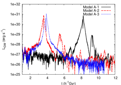
Figure 9: Comparison of luminosity evolution varying the initial relative velocity in the direction of initial separation (models A-1, A-2 and A-3).

To see the difference between these three models more closely, we plot the amplitude of the plus mode in the $z$-direction in Fig. 10. The amplitude is calculated at $10~{}h^{-1}{\rm Mpc}$ from the galaxies and the peak amplitude is of order $10^{-13}$. The difference in the amplitudes is about $20-50\%$ and increases as $\Delta V_{x}$ increases.

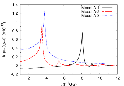
Figure 10: Amplitude of the plus mode in the $z$-direction at $10~{}h^{-1}{\rm Mpc}$ from the galaxies for models A-1, A-2 and A-3.

Fig. 11 shows the amplitude of the plus and cross modes in the $x$-, $y$- and $z$-directions for model A-2. We see that gravitational waves are mostly emitted as the plus mode in $y$- and $z$-directions, and the cross mode is smaller by one order. This comes from the fact that the galaxy motion is almost axisymmetric with respect to the $x$-axis. The small difference between radiation of the $y$- and $z$-directions is due to the small deviation of galaxy structure from the spherical symmetry.

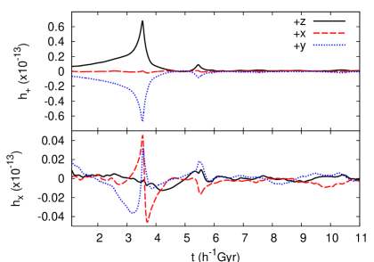
Figure 11: Amplitude of the plus (top) and cross (bottom) modes in the $x$-, $y$- and $z$-directions at $10~{}h^{-1}{\rm Mpc}$ from the galaxies for model A-2.

In Fig. 12, we show the comparison of luminosity evolution varying the initial relative velocity in the direction orthogonal to the direction of the initial separation (models B-1, B-2 and B-3). When the two galaxies have relative angular momentum, it takes more time to collide and relax into a single galaxy. Thus, the peak width broadens for large $\Delta V_{y}$ while the peak luminosity is suppressed.

Fig. 13 is the spectrum of the luminosity for models B-1, B-2 and B-3. Here the spectrum is calculated by the discrete Fourier transform,

$$\tilde{L}_{\rm GW}(f_{n})=\Delta t\sum_{k=0}^{N-1}L_{\rm GW}(t_{k})\exp\left(-\frac{2\pi ikn}{N}\right)$$ (6)

where $n=0,\cdots,N-1$ and $N$ is the number of time bins. Here $\Delta t=5/h~{}{\rm Myr}$ is the width of each time bin and $t_{k}=k\Delta t$ is the time of the $k$-th bin. Gravitational wave frequency is represented by $f_{n}=n/(N\Delta t)$. We can see that increasing $\Delta V_{y}$ decreases the characteristic frequency which corresponds to the peak width, as is expected from Fig. 12.

Relative angular momentum also affects the direction dependence of the emission. Fig. 14 shows the amplitude of the plus and cross modes in the $x$-, $y$- and $z$-directions for model B-2, which correspond to Fig. 11 for model A-2. We see that the plus and cross modes are emitted with the same order of magnitude in the $z$-direction, while there is no significant difference between model A-2 and B-2 in the $x$- and $y$-direction. This is because the galaxy motion is no longer axisymmetric, due to the relative angular momentum.

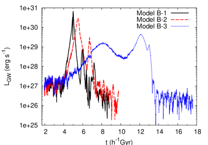
Figure 12: Luminosity evolution varying the initial relative velocity in the direction orthogonal to the direction of the initial separation (models B-1, B-2 and B-3).

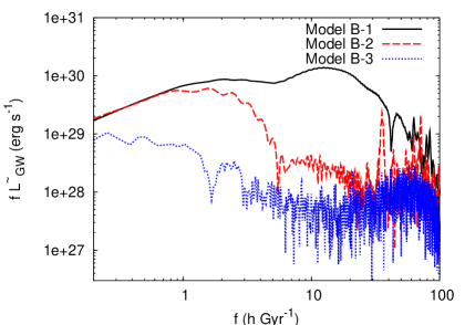
Figure 13: Fourier spectrum of the luminosity for Models B-1, B-2, B-3.

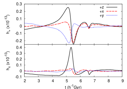
Figure 14: Amplitude of the plus (top) and cross (bottom) modes in the $x$-, $y$- and $z$-directions at $10~{}h^{-1}{\rm Mpc}$ from the galaxies for model B-2.

Fig. 15 shows the dependence of the peak luminosity as a function of the galaxy mass $M$ fixing the mass ratio to $1:1$. As can be seen, the luminosity is well fitted by $M^{10/3.4}$. One may expect that the luminosity is proportional to $M^{2}$ because the quadrupole is proportional to $M$. However, this is not the case because the length and time scales are also dependent on $M$. We can understand this behavior as follows.

Defining the typical length and time scales as $L$ and $T$, respectively, the quadrupole and luminosity are roughly given by,

$$I\sim ML^{2},~{}~{}~{}\dddot{I}\sim\frac{ML^{2}}{T^{3}},~{}~{}~{}L_{\rm GW}\sim\frac{M^{2}L^{4}}{T^{6}}.$$ (7)

On the other hand, assuming the gravitational potential energy between the two galaxies is equal to the kinetic energy of their relative motion at the collision, characteristic relative velocity $V\sim L/T$ is evaluated as,

$$V^{2}\sim 2\frac{GM}{r}\sim\frac{M}{L}.$$ (8)

Thus, we have,

$$T^{2}\sim\frac{L^{3}}{M},$$ (9)

and then,

$$L_{\rm GW}\sim\frac{M^{2}L^{4}}{T^{6}}\sim\frac{M^{5}}{L^{5}}.$$ (10)

From Eq. (5), we have $L\propto M^{1-2/\alpha}$ and finally obtain,

$$L_{\rm GW}\propto M^{\frac{10}{\alpha}},$$ (11)

with $\alpha\sim 3.4$.

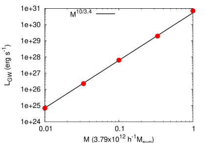
Figure 15: Peak luminosity as a function of mass fixing mass ratio to $1:1$.

Fig. 16 shows the comparison of luminosity evolution varying the mass ratio. The peak luminosity is roughly proportional to $(M_{1}/M_{2})^{1.5}$ where $M_{1}<M_{2}$. This dependence may be understood by replacing $M$ with $\sqrt{M_{1}M_{2}}$ in the discussion in the previous paragraph.

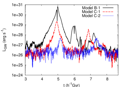
Figure 16: Luminosity evolution varying the mass ratio (models B-1, C-1 and C-2).

IV Summary and Discussion

In this paper, we performed a systematic study of gravitational waves from galaxy mergers through $N$-body simulations with Gadget2. Two types of initial condition were adopted. First we used galaxies generated by “GalactICS” which consist of disk, bulge and halo. We showed that the features of peaks such as the width and luminosity are reliably simulated with particle numbers larger than $\sim 10^{4}$. Following this, the relative importance of components was investigated and it was found that the dominant contribution to gravitational-wave luminosity comes from halo component, while contributions from other components were less than $10\%$.

Second, we used initial conditions with a dark halo adopted from a cosmological simulation. This halo had a realistic density structure and was more suitable for a precise estimation of gravitational-wave luminosity. The peak luminosity amounted to $10^{31}~{}{\rm erg~{}sec^{-1}}$ for the collision of two halos with mass $3.8\times 10^{12}~{}h^{-1}M_{\odot}$. We showed that the initial relative velocity in the direction of the initial separation does not significantly affect gravitational wave emission, with a difference of about $20-50\%$ in amplitude. On the other hand, we found that the initial relative angular momentum broadens the peak width and suppresses the luminosity by one order. Mass dependence of the peak luminosity was also investigated. In contrast to the naive expectation, $L_{\rm GW}\propto M^{2}$, we obtained $L_{\rm GW}\propto M^{3}$. We gave a simple analytic interpretation of this behavior based on the scaling relation of the mass and size of galaxies. Also this analysis was shown to be applicable to the dependence on the mass ratio.

To argue the observability of gravitational waves from galaxy merger through the B-mode polarization of CMB, it is necessary to evaluate gravitational wave background, which is contributed to by the entire history of galaxy merger. In future research we will present a detailed estimation by combining the elementary process studied here and the merger history based on hierarchical galaxy formation model Enoki et al. (2004). Here we give a very rough order-of-magnitude estimation based on several simplifying assumptions. Let us assume that all the current galaxies have mass of $10^{12}h^{-1}M_{\odot}$ and were created through successive mergers starting from the progenitor galaxies with mass $10^{10}h^{-1}M_{\odot}$. Further, we assume that all the mergers took place with mass ratio 1:1 and head-on orbit, and neglect the redshift of gravitational waves. Counting the number of mergers in the current horizon volume and multiplying the gravitational-wave energy emitted at each merger taking the scaling law in Fig. 15 into account, we obtain the density parameter of gravitational wave background as $\Omega_{\rm GW}=\rho_{\rm GW}/\rho_{\rm c}\sim 10^{-21}$ where $\rho_{\rm c}$ is the critical density. This corresponds to inflationary gravitational waves with the tensor-to-scalar ratio $\sim 10^{-6}$. Although it would be too small to be detected through B-mode polarization of CMB by the existing instruments, delensing of CMB polarization may allow us to probe such weak gravitational wave background in the future Seljak and Hirata (2004); Sigurdson and Cooray (2005).