Exact Distance Oracles for Planar Graphs

Abstract

We present new and improved data structures that answer exact node-to-node distance queries in planar graphs. Such data structures are also known as distance oracles. For any directed planar graph on $n$ nodes with non-negative lengths we obtain the following:

• Given a desired space allocation $S\in[n\lg\lg n,n^{2}]$, we show how to construct in $\tilde{O}(S)$ time a data structure of size $O(S)$ that answers distance queries in ${\tilde{O}}(n/\sqrt{S})$ time per query. The best distance oracles for planar graphs until the current work are due to Cabello (SODA 2006), Chen and Xu (STOC 2000), Djidjev (WG 1996), and Fakcharoenphol and Rao (FOCS 2001). For $\sigma\in(1,4/3)$ and space $S=n^{\sigma}$, we essentially improve the query time from $n^{2}/S$ to $\sqrt{n^{2}/S}$.

• As a consequence, we obtain an improvement over the fastest algorithm for $k$–many distances in planar graphs whenever $k\in[\sqrt{n},n)$.

• We provide a linear-space exact distance oracle for planar graphs with query time $O(n^{1/2+\epsilon})$ for any constant $\epsilon>0$. This is the first such data structure with provable sublinear query time.

• For edge lengths $\geq 1$, we provide an exact distance oracle of space ${\tilde{O}}(n)$ such that for any pair of nodes at distance $\ell$ the query time is ${\tilde{O}}(\min\{\ell,\sqrt{n}\})$. Comparable query performance had been observed experimentally but could not be explained theoretically.

Our data structures with superlinear space are based on the following new tool: given a non-self-crossing cycle $C$ with $c=O(\sqrt{n})$ nodes, we can preprocess $G$ in ${\tilde{O}}(n)$ time to produce a data structure of size $O(n\lg\lg c)$ that can answer the following queries in ${\tilde{O}}(c)$ time: for a query node $u$, output the distance from $u$ to all the nodes of $C$. This data structure builds on and provides an alternative for a related data structure of Klein (SODA 2005), which reports distances to the boundary of a face, rather than a cycle.

1 Introduction.

A fast shortest-path query data structure may be of use whenever an application needs to compute shortest-path distances between some but not necessarily all pairs of nodes. Indeed, shortest-path query processing is an integral part of many applications [Som10], in particular in Geographic Information Systems (GIS), intelligent transportation systems [JHR96]. These systems may help individuals in finding fast routes or they may also assist companies in improving fleet management, plant and facility layout, and supply chain management. A particular challenge for traffic information systems or public transportation systems is to process a vast number of queries on-line while keeping the space requirements as small as possible [Zar08]. Low space consumption is obviously very important when a query algorithm is run on a system with heavily restricted memory such as a handheld device [GW05] but it is also important for systems with memory hierarchies [HMZ03, AT05], where caching effects can have a significant impact on the query time.

While many road networks are actually not exactly planar [EG08, AFGW10], they still share many properties with planar graphs; in particular, many road networks appear to have small separators as well. For this reason, planar graphs are often used to model various transportation networks.

In the following, we provide shortest-path query data structures (also known as distance oracles) for planar graphs for essentially any specified space requirement. Throughout the paper we assume the edge lengths to be non-negative. Our results extend results of Cabello [Cab06], Chen and Xu [CX00], and Fakcharoenphol and Rao [FR06] and extend one result and improve upon another result of Djidjev [Dji96]. Consider Figure 1 for an illustration and comparison.

Theorem 1.1

Let $G$ be a directed planar graph on $n$ vertices. For any value $S$ in the range $S\in[n\lg\lg n,n^{2}]$, there is a data structure with preprocessing time $O(S\lg^{3}n/\lg\lg n)$ and space $O(S)$ that answers distance queries in $O(nS^{-1/2}\lg^{2}n\lg^{3/2}\lg n)$ time per query.

As a corollary, we obtain the following result on $k$–many distances [FMS91], improving upon an algorithm of Cabello [Cab06], which runs in time ${\tilde{O}}((kn)^{2/3}+n^{4/3})$. Our result is an improvement for $k=\tilde{o}(n)$. For the range roughly $k\in[\sqrt{n},n)$, our algorithm is faster by a factor of ${\tilde{O}}((n/k)^{2/3})$.

Theorem 1.2

Let $G$ be a directed planar graph on $n$ vertices. The distances between $k=\Omega(n^{1/2}\lg n/\lg\lg n)$ pairs of nodes $(s_{1},t_{1}),(s_{2},t_{2}),\dots(s_{k},t_{k})$ can be computed in time $O((kn)^{2/3}(\lg n)^{7/3}(\lg\lg n)^{2/3})$.

We also give a data structure that keeps the space requirements as small as possible, i.e. linear in the size of the input. This is the first linear-space data structure with provably sublinear query time for exact point-to-point shortest-path queries. Nussbaum [Nus11] has simultaneously obtained a similar result.

Theorem 1.3

For any directed planar graph $G$ with non-negative arc lengths and for any constant $\epsilon>0$, there is a data structure that supports exact distance queries in $G$ with the following properties: the data structure can be created in time $O(n\lg n)$, the space required is $O(n)$, and the query time is $O(n^{1/2+\epsilon})$.

More generally, our data structure works for the range $S\in[n,n\lg\lg n]$ (using a non-constant $\epsilon$, see details in Section 3), where we slightly improve upon the tradeoff obtained by the construction of Fakcharoenphol and Rao [FR06]. Combined with Theorem 1.1, we provide efficient distance oracles for any space bound $S\in[n,n^{2}]$.

The main techniques we use are Frederickson’s $r$–division [Fre87], Fakcharoenphol and Rao’s implementation of Dijkstra’s algorithm [FR06], and Klein’s Multiple-Source Shortest Paths (MSSP) data structure [Kle05], for which we propose a more space-efficient alternative (see Section 4 for a detailed comparison) as follows.

Theorem 1.4

Given a directed planar graph $G$ on $n$ nodes and a simple cycle $C$ with $c=O(\sqrt{n})$ nodes, there is an algorithm that preprocesses $G$ in $O(n\lg^{3}n)$ time to produce a data structure of size $O(n\lg\lg c)$ that can answer the following queries in $O(c\lg^{2}c\lg\lg c)$ time: for a query node $u$, output the distance from $u$ to all the nodes of $C$.

Since Klein’s MSSP data structure has found numerous applications, we believe that our data structure could be a rather useful tool in other algorithms as well.

The shortest-path query problem has been investigated heavily from an experimental perspective as well. Experimental results suggest that query times proportional to the shortest-path length are possible in practice using algorithms based on the so-called arc-flag technique [Lau04, KMS05, HKMS09]. Hilger, Köhler, Möhring, and Schilling make a statement about the (experimental) worst-case behavior of their method:

In all cases, the search space of our arc-flag method is never larger than ten times the actual number of nodes on the shortest paths [HKMS09, Section 6].

We can now actually prove a similar statement:

In (provably) all cases, the search space of our method is never larger than a polylogarithmic factor times the length $\ell$ of the shortest paths.

More precisely:

Theorem 1.5

For any planar graph $G$ with edge lengths $\geq 1$ there is an exact distance oracle using space $O(n\lg n\lg\lg n)$ with query time $O(\min\left\{\ell\lg^{2}\ell\lg\lg\ell,\sqrt{n}\lg^{2}n\right\})$ for any pair of nodes at distance $\ell$. The preprocessing time is bounded by $O(n^{1+\epsilon})$ for any constant $\epsilon>0$.

Note that our data structure has query time proportional to the path length. In fact, our algorithm maintains a Bellman-Ford-type invariant: after iteration $i$, the distance represents the minimum path length among all paths on ${\tilde{O}}(i)$ edges — the correct distance is computed after time roughly proportional to the minimum number of edges on a shortest path but we can only guarantee correctness after time ${\tilde{O}}(\ell)$. If we may further assume that, for some constant $\bar{\epsilon}>0$, all $s--t$ paths of length at most $(1+\bar{\epsilon})d_{G}(s,t)$ have $\Omega(h_{G}(s,t))$ edges (where $h_{G}(s,t)$ denotes the number of edges (hops) on a minimum-hop shortest-path), then our data structure can be constructed to have query time proportional to the minimum number of edges on a shortest path ${\tilde{O}}(h_{G}(s,t))$. This assumption essentially means that any $s-t$ path with significantly fewer edges than the shortest path is much longer.

Our main contributions can be summarized as follows: (i) We improve the worst-case behavior of previously known distance oracles with low space requirements, providing a distance oracle with fast preprocessing algorithm that works for the whole tradeoff curve (we also provide the first one with linear space and sublinear query time), and (ii) we make an important step towards proving the behavior observed in practice. As our main tool, (iii) we provide a more space-efficient multiple-source shortest-path data structure.

1.1 Related Work.

Shortest-path query processing for planar graphs has been studied extensively. In this section, we give a brief review of previous results. We focus on the space–query time tradeoff. See Figure 1 for a summary of known results in comparison with ours. The tradeoffs previously had not been illustrated by a space vs. query time plot as in Figure 1; indeed, the illustration suggests that a data structure like the one described in our main theorem (Theorem 1.1) was bound to exist.

Figure 1: Tradeoff of the Space [$S$] vs. the Query time [$Q$] for different shortest-path query data structures on a doubly logarithmic scale, ignoring constant and logarithmic factors. The upper line represents the $Q=n^{2}/S$ tradeoff (completely covered by oracles of Djidjev [Dji96]; the oracles of Arikati, Chen, Chew, Das, Smid, and Zaroliagis [ACC⁺96] cover the range $S\in[n^{3/2},n^{2}]$; SSSP ($S=n$) and APSP ($S=n^{2}$) also lie on this line). The lower line represents the $Q=n/\sqrt{S}$ tradeoff; the result of Djidjev [Dji96] covers the range $S\in[n^{4/3},n^{3/2}]$; Chen and Xu [CX00] and Cabello [Cab06] extend this to $S\in[n^{4/3},n^{2}]$. The data structure of Fakcharoenphol and Rao [FR06] covers the point $S=n$ and $Q=\sqrt{n}$. We extend their results to the full range.

For exact shortest-path queries, the currently best result in terms of the tradeoff between space and query time is by Fakcharoenphol and Rao [FR06]. Their data structure of space ${\tilde{O}}(n)$ can be constructed in time ${\tilde{O}}(n)$ and processes queries in time ${\tilde{O}}(\sqrt{n})$. The preprocessing time can be improved by a logarithmic factor [KMW10]. (Applications to distance oracles are not explicitly stated in [KMW10].)

Some distance oracles have better query times. Djidjev [Dji96], improving upon earlier work of Feuerstein and Marchetti-Spaccamela [FMS91], proves that, for any $S\in[n,n^{2}]$, there is an exact distance oracle with preprocessing time $O(S)$ (which increases to $O(n\sqrt{S})$ for $S\in[n,n^{3/2}]$), space $O(S)$, and query time $O(n^{2}/S)$. For a smaller range, he also proves that, for any $S\in[n^{4/3},n^{3/2}]$, there is an exact distance oracle with preprocessing time $O(n\sqrt{S})$, space $O(S)$, and query time ${\tilde{O}}(n/\sqrt{S})$. Chen and Xu [CX00], extending the range, prove that, for any $S\in[n^{4/3},n^{2}]$, there is an exact distance oracle using space $O(S)$ with preprocessing time $O(n\sqrt{S})$ and query time ${\tilde{O}}(n/\sqrt{S})$. Cabello [Cab06], mainly improving the preprocessing time, proves that, for any $S\in[n^{4/3},n^{2}]$, there is an exact distance oracle with preprocessing time and space $O(S)$ and query time ${\tilde{O}}(n/\sqrt{S})$. Compared to Djidjev’s construction, the query time is slower by a logarithmic factor but the range for $S$ is larger and the preprocessing time is faster. Nussbaum [Nus11] provides a data structure that maintains both the tradeoff from [Dji96, CX00] and the fast preprocessing time from [Cab06]. Nussbaum also provides a different data structure with a “clean” tradeoff of space $O(S)$ and query time $O(n/\sqrt{S})$, however spending time ${\tilde{O}}(S^{3/2}/\sqrt{n})$ in the preprocessing phase. In our construction, we sacrifice another root-logarithmic factor in the query time (compared to [Cab06]) but we prove the bounds for essentially the whole range of $S$; our preprocessing time remains ${\tilde{O}}(S)$.

If constant query time is desired, storing a complete distance matrix is essentially the best solution we have. Wulff-Nilsen [WN10a] recently improved the space requirements to $o(n^{2})$. If the space is restricted to linear, using the linear-time single-source shortest path algorithm of Henzinger, Klein, Rao, and Subramanian [HKRS97] is the fastest known for exact shortest-path queries until the current work (Theorem 1.3). Nussbaum [Nus11] has simultaneously obtained a result similar to Theorem 1.3.

Efficient data structures for shortest-path queries have also been devised for restricted classes of planar graphs [DPZ00, CX00] and for restricted types of queries [Epp99, KK06, Sch98, Kle05]. If approximate distances and shortest paths are sufficient, a better tradeoff with ${\tilde{O}}(n)$ space and ${\tilde{O}}(1)$ query time has been achieved [Tho04, Kle02, Kle05, KKS11].

Based on separators, geometric properties, and other characteristics such as highway structures, many efficient practical methods have been devised [GSSD08, SS05, BFSS07], their time and space complexities are however difficult to analyze. Competitive worst-case bounds have been achieved under the assumption that actual road networks have small highway dimension [AFGW10, ADF⁺11]. While our preprocessing algorithm (Theorem 1.5) runs in almost linear time, some of the problems that appear in the preprocessing stage of practical route planning methods have recently been proven to be NP-hard [BDDW09, BCK⁺10].

2 Preliminaries.

2.1 Recursive $r$–division of Planar Graphs.

Let $G=(V,E)$ be a planar graph with $|V|=n$. Let $E_{P}$ be a subset of $E$, and let $P=(V_{P},E_{P})$ be the subgraph of $G$ induced by $E_{P}$. $P$ is called a piece of $G$. The nodes of $V_{P}$ that are incident in $G$ to nodes of $V\setminus V_{P}$ are called the boundary nodes of $P$ and denoted by $\partial P$.

An $r$–division [Fre87] of $G$ is a decomposition into $O(n/r)$ edge-disjoint pieces, each with $O(r)$ nodes and $O(\sqrt{r})$ boundary nodes. We use an $r$–division with the additional property that, in each piece, there exist a constant number of faces, called holes, such that every boundary node is incident to some hole. Such a decomposition can be found in $O(n\lg r+nr^{-1/2}\lg n)$ [WN10b] by applying Miller’s cycle separator [Mil86] iteratively.

We use this $r$–division recursively. Let the base of the recursion be level $0$, and let the top of the recursion be level $k$. The entire graph $G$ is defined to be the only piece at level $k$. The pieces of level $i$ of the recursion are obtained by computing an $r_{i}$–division for each level–$(i+1)$ piece. The notation $r_{i}$ suggests that we may use a different parameter $r$ in the $r$–division at every level of the recursion. Indeed, using a non-uniform recursion is important in obtaining Theorem 1.3. For a level–$i$ piece $P$, the level–$(i-1)$ pieces obtained by applying the $r$–division to $P$ are called the subpieces of $P$.

We stress that the classification of nodes of a piece at any level as boundary nodes is with respect to $G$ (and not $P$). This implies that, if $v$ is a boundary node of a level–$i$ piece, then $v$ is also a boundary node of any lower-level piece that contains $v$. This generalizes the decomposition used in [FR06], where Miller’s separator is used at each level rather than an $r$–division.

2.2 Klein’s Multiple-Source Shortest Paths Algorithm.

Klein [Kle05] gave a multiple-source shortest path (MSSP) algorithm with the following properties. The input consists of a directed planar embedded graph $G$ with non-negative arc-lengths, and a face $f$. For each node $u$ in turn on the boundary of $f$, the algorithm computes (an implicit representation of) the shortest-path tree rooted at $u$. This takes a total of $O(n\lg n)$ time and space. Subsequently, the distance between any pair $(u,v)$ of nodes of $G$ where $u$ is on the boundary of $f$ (and $v$ is an arbitrary node), can be queried in $O(\lg n)$ time. In particular, given a set $S$ of $O(\sqrt{n})$ nodes on the boundary of a single face, the algorithm can compute all $S$-to-$S$ distances in $O(n\lg n)$ time.

We propose a more space-efficient alternative in Section 4, wherein we also provide a detailed comparison.

2.3 Dense Distance Graphs and Efficient Implementation of Dijkstra’s Algorithm.

The dense distance graph for a piece $P$, denoted by $DDG_{P}$, is the complete graph on $\partial P$, the boundary nodes of $P$, such that the length of an arc corresponds to the distance (in $P$) between its endpoints. The dense distance graph for all pieces $P$ in the $r$–division can be computed in $O(|V(G)|\lg|V(G)|)$ time and space using Klein’s MSSP; For each piece $P$, compute MSSP data structures in $O(|P|\lg|P|)$ time and space a constant number of times, specifying a different hole of $P$ as the distinguished face at each run. Then query the MSSP data structures for the distances between the boundary nodes in $O(|\partial P|^{2}\lg|P|)$ time. Since in an $r$–division $|\partial P|=\sqrt{|P|}$, this takes $O(|P|\lg|P|)$ time and space per piece, for a total of $O(|V(G)|\lg|V(G)|)$ for all pieces.

Let ${\mathcal{P}}$ be a set of pieces (not necessarily at the same level), and let the graph $H$ be the union of the dense distance graphs of the pieces in ${\mathcal{P}}$. Fakcharoenphol and Rao [FR06] devised an ingenious implementation of Dijkstra’s algorithm [Dij59] that computes a shortest-path tree in $H$ in time $O(|V(H)|\lg^{2}n)$, where $|V(H)|$ is the number of nodes in $H$ (i.e., the total number of boundary nodes in all the pieces in ${\mathcal{P}}$). We will refer to this implementation as FR-Dijkstra.

In fact, the proof of Fakcharoenphol and Rao’s algorithm only relies on the property that the distances in each of the dense distance graphs given as input correspond to distances in a planar graph between a set of nodes that lie on a constant number of faces. It does not rely on any other properties of the $r$–division.

FR-Dijkstra can be extended to the following setting (cf. [BSWN10]). Let $J$ be a planar graph. Let $n^{\prime}$ denote the number of nodes of $J\cup H$. We can compute shortest paths in $H\cup J$ in $O(|H|\lg^{2}|H|+n^{\prime}\lg n^{\prime})$ time. The edges of $H$ are relaxed using FR-Dijkstra, while the edges of $J$ are relaxed as in a traditional implementation of Dijkstra’s algorithm using a heap.

2.3.1 External Dense Distance Graphs.

For a piece $P$, let $G-P$ be the graph obtained from $G$ by deleting the nodes in $V_{P}-\partial P$. The external dense distance graph of $P$, denoted by $DDG_{G-P}$, is the complete graph on $\partial P$ such that the length of an arc corresponds to the distance between its endpoints in $G-P$. External dense distance graphs were used recently in [BSWN10]. Computing the external dense distance graphs for all pieces in an $r$–division cannot be done efficiently using Klein’s MSSP. The reason is that $|V(G-P)|$ can be $\Theta(|V(G)|)$ for all pieces. Instead, the computation can be done in a top-down approach as follows (cf. [BSWN10]). Recall that an $r$–division is obtained as the set of pieces of the lowest level in a recursive division of the graph using Miller’s simple-cycle separators. Consider the set ${\mathcal{Q}}$ of all pieces at all levels of the recursion (rather than just the set of pieces at the lowest level). Note that there are $O(\lg|V(G)|)$ recursive levels since the size of the pieces decreases by a constant factor for every constant number of applications of Miller’s cycle separator theorem. First, we compute $DDG_{Q}$ for every piece $Q\in{\mathcal{Q}}$. As explained above, this can be done in $O(|V(G)|\lg|V(G)|)$ for all the pieces in a specific level of the recursion, for a total of $O(|V(G)|\lg^{2}|V(G)|)$ for all pieces in ${\mathcal{Q}}$. Next, we consider a piece $Q$ and denote the two subpieces of $Q$ by $Q_{1}$ and $Q_{2}$. $DDG_{G-{Q_{2}}}$ is obtained by computing distances in $DDG_{Q_{1}}\cup DDG_{G-Q}$ (see Figure 2), using multiple applications of FR-Dijkstra, once for each node in $\partial Q_{2}$. This takes $O(|Q|\lg^{2}|\partial Q|)$ time per piece, for an overall $O(|V(G)|\lg^{2}|V(G)|)$ time for all pieces in a specific level. Since the number of levels is bounded by $O(\lg|V(G)|)$, the entire computation takes $O(|V(G)|\lg^{3}|V(G)|)$ time.

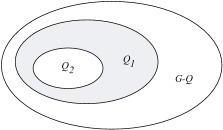
Figure 2: Pieces $Q_{1}$ and $Q_{2}$ in some level of the recursive application of Miller’s cycle separator theorem. The piece $Q$ is the union of $Q_{1}$ and $Q_{2}$. Distances in $G-Q_{2}$, the exterior of $Q_{2}$, are obtained by considering shortest paths in the interior of $Q_{1}$ and in $G-Q$, the exterior of $Q$.

3 A Linear-Space Distance Oracle.

We first provide our linear-space data structure. The techniques employed here are reused in the subsequent sections, particularly in the cycle MSSP data structure (Section 4). In the following we prove a more precise version of Theorem 1.3.

Theorem 1.3

For any directed planar graph $G$ with non-negative arc lengths and for any constant $\epsilon>0$, there is a data structure that supports exact distance queries in $G$ with the following properties: the data structure can be created in time $O(n\lg n)$, the space required is $O(n)$, and the query time is $O(n^{1/2+\epsilon})$.

For non-constant $\epsilon>0$, the preprocessing time is $O(n\lg(n)\lg({1/\epsilon}))$, the space required is $O(n\lg({1/\epsilon}))$, and the query time is $O(n^{1/2+\epsilon}+n^{1/2}\lg^{2}(n)\lg({1/\epsilon}))$.

Our distance oracle is an extension of the oracle in Fakcharoenphol and Rao [FR06]. The main ingredients of our improved space vs. query time tradeoff are (i) using recursive $r$–divisions instead of cycle separators, and (ii) using an adaptive recursion, where the ratio between the boundary sizes of piece at consecutive levels is $\sqrt{n}$.

We split the proof into descriptions and analysis of the preprocessing and query algorithms. Let $k=\Theta(\lg(1/\epsilon))$.

Preprocessing.

We compute the recursive $r$–division of the graph with $k$ recursive levels and values of $\{r_{i}\}_{i=0}^{k}$ to be specified below. This takes $O(kn\lg n)$ time. We then compute the dense distance graph for each piece. This is done for a piece $P$, with $r$ nodes and $O(\sqrt{r})$ boundary nodes on a constant number of holes, by applying Klein’s MSSP algorithm [Kle05] as described in Section 2.3. Thus, all of the boundary-to-boundary distances in $P$ are computed in $O(r\lg r)$ time. Summing over all $O(n/r_{i})$ pieces at level $i$, the preprocessing time per level is $O(n\lg r_{i})$. The overall time to compute the dense distance graphs for all pieces over all recursive levels is therefore $O(kn\lg n)$.

The space required to store $DDG_{P}$ is $O((\sqrt{r})^{2})=O(r)$; summing over all pieces at level $i$ we obtain space $O(\frac{n}{r_{i}}r_{i})=O(n)$ per level; the total space requirement is $O(kn)$.

Query.

Given a query for the distance between nodes $u$ and $v$, we proceed as follows. For simplicity of the presentation, we initially assume that neither $u$ nor $v$ are boundary nodes.

Let $P_{0}$ be the level–$0$ piece that contains $u$. We compute distances from $u$ in $P_{0}$. This is done in $O(r_{0})$ time using the algorithm of Henzinger et al. [HKRS97]. Denote these distances by $\textrm{dist}_{P_{0}}(u,w)$ for $w\in P_{0}$. Let $H_{0}$ denote the star graph with center $u$ and leaves $w\in\partial P_{0}$. The arcs of $H_{0}$ are directed from $u$ to the leaves, and their lengths are the corresponding distances in $P_{0}$.

Let $S_{u}$ be the set of pieces that contain $u$. Note that $S_{u}$ contains exactly one piece of each level. Let $R_{u}$ be the union of subpieces of every piece in $S_{u}$. That is, $R_{u}=\bigcup_{P\in S_{u}}\{P^{\prime}:P^{\prime}\textrm{ is a subpiece of }P\}$. Let $H_{u}$ be the union of the dense distance graphs of the pieces in $R_{u}$. We use FR-Dijkstra (see Section 2.3) to compute distances from $u$ in $H_{u}\cup H_{0}$. Observe that any shortest path from $u$ to a node of $H_{u}$ can be decomposed into a shortest path in $P_{0}$ from $u$ to $\partial P_{0}$ and shortest paths each of which is between boundary nodes of some piece in $R_{u}$. Since all $u$-to-$\partial P_{0}$ shortest paths in $P_{0}$ are represented in $H_{0}$, and since all shortest paths between boundary nodes of pieces in $R_{u}$ are represented in $H_{u}$, this observation implies that distances from $u$ to nodes of $H_{u}$ in $H_{u}\cup H_{0}$ are equal to distances from $u$ to nodes of $H_{u}$ in $G$. We denote these distances by $\textrm{dist}_{G}(u,w)$ for nodes $w\in H_{u}$.

We repeat a similar procedure for $v$ (reversing the direction of arcs) to compute $\textrm{dist}_{G}(w,v)$, the distances in $G$ from every node $w\in H_{v}$ to $v$.

Let $P_{uv}$ be the lowest-level piece that contains both $u$ and $v$. Assume first that $P_{uv}$ is not a level–$0$ piece. Let $P_{u}$ ($P_{v}$) be the subpiece of $P_{uv}$ that contains $u$ ($v$). Since $P_{uv}$ is both in $S_{u}$ and in $S_{v}$, both $P_{u}$ and $P_{v}$ are in $R_{u}$ as well as in $R_{v}$. This implies that we have already computed $\textrm{dist}_{G}(u,w)$ and $\textrm{dist}_{G}(w,v)$ for all $w\in\partial P_{u}$. Since we have assumed that $P_{uv}$ is not a level–$0$ piece, the shortest $u$-to-$v$ path must contain some node of $\partial P_{u}$. Therefore, the $u$-to-$v$ distance can be found by computing

$$\min_{w\in\partial P_{u}}\textrm{dist}_{G}(u,w)+\textrm{dist}_{G}(w,v).$$

If $P_{uv}$ is a level–$0$ piece, then $P_{uv}=P_{0}$ , and the $u$-to-$v$ distance can be found by computing

$$\min\left\{\textrm{dist}_{P_{0}}(u,v),\min_{w\in\partial P_{uv}}\{\textrm{dist}_{G}(u,w)+\textrm{dist}_{G}(w,v)\}\right\}.$$

The case when $u$ or $v$ are boundary nodes is a degenerate case that can be solved by the above algorithm. Let $Q_{u}$ be the highest-level piece of which $u$ is a boundary node. We have the preprocessed distances in $Q_{u}$ from $u$ to all other nodes of $\partial{Q_{u}}$. Therefore, it suffices to replace $S_{u}$ above with the set of pieces that contain $Q_{u}$ as a subgraph in order to assure that $H_{u}$ is small enough and that the distances computed by the fast implementation of Dijkstra’s algorithm are the distances from $u$ to nodes of $H_{u}$ in $G$.

Query Time.

Computing the distances $\textrm{dist}_{P_{0}}(\cdot,\cdot)$ takes $O(r_{0})$ time. Let $|V(H_{u})|$ denote the number of nodes of $H_{u}$. The FR-Dijkstra implementation runs in $O(|V(H_{u})|\lg^{2}n)$ time. It therefore remains to bound $|V(H_{u})|$. Let $P_{i}$ be the level–$i$ piece in $S_{u}$. $P_{i}$ has $O(\frac{r_{i}}{r_{i-1}})$ subpieces, each with $O(\sqrt{r_{i-1}})$ boundary nodes. Therefore, the contribution of $P_{i}$ to $|V(H_{u})|$ is $O(\frac{r_{i}}{\sqrt{r_{i-1}}})$. The total running time is therefore

$$O\left(r_{0}+\lg^{2}n\sum_{i=1}^{k}\frac{r_{i}}{\sqrt{r_{i-1}}}\right).$$

Recall that $r_{k}=|V(G)|=n$, and set $r_{0}=\sqrt{n}$. For $i=1\dots k-1$ we recursively define $r_{i}$ so as to satisfy

$$\frac{r_{i}}{\sqrt{r_{i-1}}}=\sqrt{n}.$$

This implies

$$r_{1} = n^{\frac{1}{2}+\frac{1}{4}}=n^{1-\frac{1}{4}}$$

$$r_{2} = n^{\frac{1}{2}+\frac{3}{8}}=n^{1-\frac{1}{8}}$$

$$r_{3} = n^{\frac{1}{2}+\frac{7}{16}}=n^{1-\frac{1}{16}}$$

$$\ldots$$

$$r_{k-1} = n^{1-\frac{1}{2^{k}}}.$$

The total running time is thus bounded by

$$O\left(\sqrt{n}+\lg^{2}n\left((k-1)\sqrt{n}+\frac{n}{\sqrt{n^{1-\frac{1}{2^{k}}}}}\right)\right) \leq$$

(3.1) $$O\left(\left(k\sqrt{n}+n^{\frac{1}{2}+\frac{1}{2^{k+1}}}\right)\lg^{2}n\right).$$

By setting $k=\Theta(\lg(1/\epsilon))$ we obtain the claimed running times.

4 A Cycle MSSP Data Structure for Planar Graphs.

In this section we provide our main technical tool. We prove Theorem 1.4, which we restate here.

Theorem 1.4

Given a directed planar graph $G$ on $n$ nodes and a simple cycle $C$ with $c=O(\sqrt{n})$ nodes, there is an algorithm that preprocesses $G$ in $O(n\lg^{3}n)$ time to produce a data structure of size $O(n\lg\lg c)$ that can answer the following queries in $O(c\lg^{2}c\lg\lg c)$ time: for a query node $u$, output the distance from $u$ to all the nodes of $C$.

Comparison with Klein’s MSSP data structure

Our data structure can be seen as an alternative to Klein’s MSSP data structure (see Section 2.2) with two main advantages (which we exploit in Section 5):

• our data structure can handle queries to any not-too-long cycle as opposed to a single face (the crucial difference and difficulty is that shortest paths may cross a cycle but not a face),

• the space requirements are only $O(n\lg\lg c)$ (we internally rely on the data structure in Theorem 1.3, so even $O(n)$ is possible at the cost of increasing the query time) as opposed to $O(n\lg n)$,

and three main disadvantages:

• our data structure cannot efficiently answer queries from $u$ to a single node on the cycle $C$; such a query requires the same time as computing the distances from $u$ to all the nodes on $C$ (in many existing applications, this disadvantage is not really problematic, since MSSP is used for all nodes on the face anyway),

• our data structure requires amortized time $O(\lg^{2}c\lg\lg c)$ per node on the cycle (as opposed to $O(\lg n)$), which is slower for long cycles, and

• the preprocessing time of our data structure is $O(n\lg^{3}n)$ as opposed to $O(n\lg n)$.

Let $G$ be an embedded planar graph.

Preprocessing.

Let $G_{0}$ be the exterior of $C$. That is, the graph obtained from $G$ by deleting all nodes strictly enclosed by $C$. Consider $C$ as the infinite face of $G_{0}$. Similarly, let $G_{1}$ be the interior of $G$. Namely, the graph obtained from $G$ by deleting all nodes not enclosed by $C$. Consider $C$ as the infinite face of $G_{1}$. Note that we have reduced the problem from query nodes on a cycle $C$ to query nodes on a face. The query algorithm is supposed to handle paths that cross $C$. The preprocessing step consists of the following:

1. Computing $DDG_{C}$ and $DDG_{G-C}$. This can be done in $O((n+c^{2})\lg n)$ time using Klein’s MSSP algorithm [Kle05]. Storing $DDG_{C}$ and $DDG_{G-C}$ requires $O(c^{2})=O(n)$ space.

2. Computing an $r$–division of $G_{i}$ ($i\in\{0,1\}$) with $r=c^{2}$. Each piece has $O(c^{2})$ nodes and $O(c)$ boundary nodes incident to a constant number of holes. Consider all the nodes of $C$ as boundary nodes of every piece in the division. Note that each piece still has $O(c)$ boundary nodes. This step takes $O(n\lg n)$ time.

3. Computing, for each piece $P$, a recursive $r$–division of $P$ as the one in the preprocessing step of the oracle in Section 3 (Theorem 1.3) with $\epsilon=1/\lg c$. That is, the number of levels in this recursive $r$–division is $k=\Theta(\lg\lg c)$. The top-level (level–$k$) piece in this recursive division is the entire piece $P$. In the description in Section 3, the top-level piece is the entire graph and therefore it has no boundary nodes. Here, in contrast, we consider the boundary nodes of $P$ as boundary nodes of the top-level piece in the decomposition (and thus, as boundary nodes of any lower-lever piece in which they appear). This does not asymptotically change the total number of boundary nodes at any level of the recursive decomposition since $P$ has $O(c)$ boundary nodes, and every level of the recursive decomposition consists of a total of $\Omega(c)$ boundary nodes. The time to compute the recursive $r$–division for all pieces is bounded by $O(n\lg^{2}n)$.

4. Computing, for each piece $P$, the dense distance graph for each of the pieces in the recursive decomposition of $P$. Let $H_{P}$ denote the union of the dense distance graphs for all the pieces in the recursive decomposition of $P$. As discussed in Section 3, the space required to store $H_{P}$ is $O(|P|\lg\epsilon)=O(|P|\lg\lg c)$. Using the methods presented in Section 3, computing $H_{P}$ takes $O(|P|\lg|P|\lg\lg c)=O(c^{2}\lg c\lg\lg c)$. Thus, the total space and time required over all pieces $P$ is $O(n\lg\lg c)$ and $O(n\lg c\lg\lg c)$, respectively.

5. Computing, for each piece $P$, the dense distance graph $DDG_{G_{i}-P}$. Recall that we consider the nodes of $C$ as boundary nodes of every piece in the division. These dense distance graphs can be computed as described in Section 2.3.1. As shown there, the entire computation (for all pieces combined) takes $O(n\lg^{3}n)$ time.

The time required for the preprocessing step is therefore $O(n\lg^{3}n)$ and the space required is $O(n\lg\lg c)$.

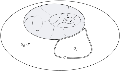
Figure 3: A schematic diagram showing the various subgraphs whose dense distance graphs are used in a query to the cycle MSSP data structure. The cycle $C$ is double-lined. The interior of $C$ is the subgraph $G_{1}$. The query node $u$ is indicated by a small solid circle. The piece $P$ in the $r$–division of the exterior of $C$ ($G_{0}$) is shown as a grey region with solid boundary. The boundaries of the pieces whose dense distance graphs are in $H_{u}$ are shown as dotted lines (one level) and dashed-dotted lines (another level). $P_{0}$ is the smallest piece of $P$ that contains $u$. Any shortest path from $u$ to $C$ can be decomposed into a shortest path from $u$ to $\partial P_{0}$ followed by shortest paths between nodes on the boundaries shown in the figure.

Query.

When queried with a node $u$, the data structure outputs the distances from $u$ to all the nodes of $C$. We describe the case where $u$ is not enclosed by $C$. In this case, we use the dense distance graphs computed in the preprocessing step for $G_{0}$. The symmetric case is handled similarly, by using the dense distance graphs computed for $G_{1}$.

Let $P$ be the piece in the $r$–division of $G_{0}$ to which $u$ belongs. Recall that $P$ consists of $O(c^{2})$ nodes. Consider the recursive $r$–division of $P$ computed in item 3 of the preprocessing stage. Let $P_{0}$ be the level–$0$ piece of $P$ that contains $u$. $P_{0}$ consists of $O(\sqrt{c^{2}})=O(c)$ nodes.

We first compute [HKRS97], in $O(c)$ time, the distances from $u$ to all nodes of $P_{0}$, and store them in a table $\textrm{dist}_{P_{0}}$. We then compute, using FR-Dijkstra, the distances from $u$ in the union of the following dense distance graphs (see Figure 3):

1. $H_{0}$, the star graph with center $u$ and leaves $\partial P_{0}$. The arcs of $H_{0}$ are directed from $u$ to the leaves and their lengths are the corresponding lengths in $\textrm{dist}_{P_{0}}$.

2. $H_{u}$, the subset of dense distance graphs in $H_{P}$ that correspond to pieces in the recursive decomposition of $P$ that contain $u$ and their subpieces. These dense distance graphs are available in $H_{u}$.

3. $DDG_{G_{0}-P}$

4. $DDG_{C}$

Note that the first two graphs are the analogs of $H_{0}$ and $H_{u}$ from Section 3.

Distances from $u$ in the union of the above graphs are equal to the distances from $u$ in $G$. This is true since any $u$-to-$C$ shortest path can be decomposed into (i) a shortest path in $P_{0}$ from $u$ to $\partial P_{0}$, (ii) shortest paths each of which is a shortest path in $Q$ between boundary nodes of $Q$ for some piece $Q$ in the recursive $r$–division of $P$ that is represented in $H_{u}$, (iii) shortest paths in $G_{0}-P$ between nodes of $\partial P\cup C$, and (iv) shortest paths in the interior of $C$ between nodes of $C$.

To bound the running time of FR-Dijkstra we need to bound the number of nodes in all dense distance graphs used in the FR-Dijkstra computation. $H_{0}$ has $O(\sqrt{c})$ nodes. The analysis in Section 3 shows that the graphs in the set $H_{u}$ consist of $O(\sqrt{|P|}\lg\lg|P|)$ nodes (substitute $k=1/\lg|P|$ in eq. (3)). $DDG_{G_{0}-P}$ has $O(c+\sqrt{|P|})=O(c)$ nodes, and $DDG_{C}$ has $c$ nodes. Combined, the running time of the invocation of FR-Dijkstra is bounded by $O(c\lg^{2}c\lg\lg c)$. This dominates the $O(c)$ time required for the computation of $\textrm{dist}_{P_{0}}$, so the overall query time is $O(c\lg^{2}c\lg\lg c)$, as claimed.

5 Distance Oracles with Space $S\in[n\lg\lg n,n^{2}]$.

In this section we prove Theorem 1.1. Using our new cycle MSSP data structure, the proof is rather straightforward.

Theorem 1.1

Let $G$ be a directed planar graph on $n$ vertices. For any value $S$ in the range $S\in[n\lg\lg n,n^{2}]$, there is a data structure with preprocessing time $O(S\lg^{3}n/\lg\lg n)$ and space $O(S)$ that answers distance queries in $O(nS^{-1/2}\lg^{2}n\lg^{3/2}\lg n)$ time per query.

• Let $r:=(n^{2}\lg\lg n)/S$. Note that $r\in[\lg\lg n,n]$ for any $S\in[n\lg\lg n,n^{2}]$.
  

Preprocessing.

We start by computing an $r$–division. Each piece has $O(r)$ nodes and $O(\sqrt{r})$ boundary nodes incident to a constant number of holes. For each piece $P$ we compute the following:

1. A distance oracle as in Theorem 1.3 with $\epsilon=1/\lg r$. This takes $O(r\lg r\lg\lg r)$ time and $O(r\lg\lg r)$ space.

2. For each hole of $P$ (bounded by a cycle in $G$) we compute our new cycle MSSP data structure. Since the number of holes per piece is constant, this requires requires $O(n\lg^{3}n)$ time and $O(n\lg\lg n)$ space per piece.

Summing over all pieces, the preprocessing time is $O(S\lg^{3}n/\lg\lg n)$ and the space needed is $O(S)$.

Query.

Given a pair of nodes $(s,t)$, we compute a shortest $s$–$t$ path as follows. Assume first that $s$ and $t$ are in different pieces. Let $P$ denote the piece that contains $s$ and let $\partial P$ denote its boundary. We compute the distances in $G$ from $\partial P$ to $t$ using the cycle MSSP data structures. These distances can be obtained in time $O(|\partial P|\lg^{2}n\lg\lg n)=O(\sqrt{r}\lg^{2}n\lg\lg n)$. Analogously, we compute the distances in $G$ from $s$ to $\partial P$. It remains to find the node $p\in\partial P$ that minimizes $d_{G}(s,p)+d_{G}(p,t)$, which can be done in $O(|\partial P|)=O(\sqrt{r})$ time using a simple sequential search.

If $s$ and $t$ lie in the same piece, the shortest $s$–$t$ path might not visit $\partial P$. To account for this, we query the distance oracle for $P$, which takes $O(\sqrt{r}\lg^{2}r\lg\lg r)$ time. We return the minimum distance found. $\Box$

$k$–many distances

As a consequence, we also obtain an improved algorithm for $k$–many distances, whenever $k=\Omega(\sqrt{n}/\lg\lg n)$.

• [of Theorem 1.2] For some value of $r$ to be specified below, we preprocess $G$ in time $O((n^{2}/r)\lg^{3}n)$, and then we answer each of the $k$ queries in time $O(\sqrt{r}\lg^{2}r\lg\lg r)$. The total time is $O((n^{2}/r)\lg^{3}n+k\sqrt{r}\lg^{2}r\lg\lg r)$. This is minimized by setting $r=n^{4/3}k^{-2/3}(\lg n/\lg\lg n)^{2/3}$. Note that $r=O(n)$ since $k=\Omega(\sqrt{n}\lg n/\lg\lg n)$. The total running time is thus $O((kn)^{2/3}(\lg n)^{7/3}(\lg\lg n)^{2/3})$. $\Box$

Comparison and Discussion.

The query time of our data structure is at most $O(\sqrt{r}\lg^{2}r\lg\lg r)$, which, in terms of $S$, is $O(nS^{-1/2}\lg^{2}n\lg^{3/2}\lg n)$. Let us contrast this with Cabello’s data structure [Cab06] that, for any $S\in[n^{4/3}\lg^{1/3}n,n^{2}]$ has preprocessing time and space $O(S)$ and query time $O(nS^{-1/2}\lg^{3/2}n)$. In our construction, we sacrifice a factor of $O(\sqrt{\lg n(\lg\lg n)^{3}})$ in the query time but we gain a much larger regime for $S$. For the range $S\in[\omega(n\lg n/\lg\lg n),o(n^{4/3}\lg^{1/3}n)]$, only data structures of size $O(S)$ with query time $O(n^{2}/S)$ had been known [Dji96] (see also Figure 1).

To conclude this section, let us observe what happens when we gradually decrease the space requirements $S$ from $n^{2}$ down to $n$, and, en passant, let us pose some open questions. For quadratic space (or even slightly below [WN10a]), we can obtain constant query time. As soon as we require the space to be $O(n^{2-\epsilon})$ for some $\epsilon>0$, the query time increases from constant or poly-logarithmic to a polynomial. It is currently not known whether ${\tilde{O}}(1)$ is possible or not — the known lower bounds [SVY09, PR10] on the space of distance oracles work for non-planar graphs only. Further restricting the space, as long as the space available is at least $\Omega(n\lg n)$, the data structure can internally store MSSP data structures. The query time for this regime of $S$ can actually be made slightly faster than what we claim in Theorem 1.1 (by avoiding the $O(\lg\lg n)$–factor due to the recursion needed in Theorem 1.3 and its manifestation in the cycle MSSP data structure). The data structure of Nussbaum [Nus11] obtains a “clean” tradeoff with query time proportional to $O(n/\sqrt{S})$ for $S\geq n^{4/3}$ (without logarithmic factors in the query time, currently at the cost of a slower preprocessing algorithm). The obvious open question is whether it is possible to obtain a data structure with space $O(S)$ and query time $O(n/\sqrt{S})$ for the whole range of $S\in[n,n^{2}]$ and without substantial sacrifices with respect to the preprocessing time. Another open question is whether it is possible to improve upon this tradeoff. Note that, for quadratic space, an improvement of an (almost) logarithmic factor is possible [WN10a].

As soon as we require the space to be $o(n\lg n)$, we cannot afford to store the MSSP data structure anymore and we are currently forced to rely on the cycle MSSP data structure (Theorem 1.4). The query time increases to the time bound claimed in Theorem 1.1. When we further restrict the space to $o(n\lg\lg n)$, say $S=\Theta(n\lg(1/\epsilon))$ for some $\epsilon>0$, the query time increases to $O(n^{1/2+\epsilon})$. A different recursion (maybe à la [HKRS97]) could potentially reduce this to ${\tilde{O}}(\sqrt{n})$.

Let us briefly consider the additional space of the data structure, assuming that storing the graph is free. It is known that, for approximate distances, a query algorithm can run efficiently using a data structure that occupies sublinear additional space [KKS11]. For exact distances and sublinear space, nothing better than the linear-time SSSP algorithm [HKRS97] is known.

6 Distance Oracles with Query Time Quasi-Proportional to the Shortest-Path Length

We use our new cycle MSSP data structure to prove Theorem 1.5, which states that there is a distance oracle with query time proportional to the shortest-path length. We actually prove two versions, the stronger one being a distance oracle with query time proportional to the minimum number of edges (hops) on a shortest path. For the stronger version, we need the following assumption, which essentially means that approximate shortest paths do not use significantly fewer edges.

Assumption 6.1

Let $h_{G}(s,t)$ denote the number of edges on a minimum-hop shortest-path. For some constant $\bar{\epsilon}>0$, all $s$–$t$ paths of length at most $(1+\bar{\epsilon})d_{G}(s,t)$ have $\Omega(h_{G}(s,t))$ edges.

We restate Theorem 1.5 and its stronger variant.

Theorem 1.5

For any planar graph $G$ with edge lengths $\geq 1$ there is an exact distance oracle using space $O(n\lg n\lg\lg n)$ with query time $O(\min\left\{\ell\lg^{2}\ell\lg\lg\ell,\sqrt{n}\lg^{2}n\right\})$ for any pair of nodes at distance $\ell$. The preprocessing time is bounded by $O(n^{1+\epsilon})$ for any constant $\epsilon>0$.

Furthermore, if Assumption 6.1 holds for $G$, the query time is at most $O(\min\left\{h\lg^{2}h\lg\lg h,\sqrt{n}\lg^{2}n\right\})$ for any pair of nodes $(u,v)$ at hop-distance $h=h_{G}(u,v)$.

Our main ingredient is a distance oracle for planar graphs with tree-width $w$.

Theorem 6.1

Let $G$ be a planar graph on $n$ vertices with tree-width $w$. For any constant $\epsilon>0$ and for any value $S$ in the range $S\in[n\lg\lg w,n^{2}]$, there is a data structure with preprocessing time $O(S\lg^{2}n+n^{1+\epsilon})$ and space $O(S)$ that answers distance queries in $O(\min\{nS^{-1/2}\lg^{2.5}n,w\lg^{2}w\lg\lg w\})$ time per query.

Note that for $S$ superlinear in $n$ but less than roughly $nw$, the oracle cannot make any use of the additional space available and the query algorithm runs in time proportional to $w$ (up to logarithmic factors). Any application should use either space close to linear or more than $\Omega(nw)$.

Using Theorem 6.1, the proof of Theorem 1.5 boils down to a combination of slicing (see for example [Bak94, Kle08]), local tree-width [Epp00, DH04], and scaling.

• [of Theorem 1.5] We repeatedly use Theorem 6.1 for different subgraphs as follows.

Slicing and local tree-width.

We use standard techniques [Bak94, Kle08] and research on the related linear local tree-width property [Epp00, DH04] to slice a planar graph into subgraphs of a certain tree-width:

• We compute a breadth-first search tree in the planar dual rooted at an arbitrary face.

• The subgraph induced by the nodes at depth $d\in[d_{1},d_{2}]$ has tree-width $O(d_{2}-d_{1})$ [Epp00, DH04].

If we were only interested in paths using at most $w$ edges, we could (i) cut the graph into slices of depth $w$, and (ii) check the union of any two consecutive levels containing both endpoints. It is straightforward to see that each path on $w$ edges lies completely within one of these unions.

Scaling.

We apply the slicing step described in the previous paragraph for different scales.

• For every integer $i>0$ with $2^{i}\leq\sqrt{n}$, we slice the graph into subgraphs $G^{i}_{j}$ at depth $r=2^{i}$; here, $G^{i}_{j}$ denotes the graph induced by the nodes adjacent to all the faces at depth in $[jr,(j+1)r)$. Every subgraph $G^{i}_{j}$ has tree-width at most $O(r)$.

• For any two consecutive $G^{i}_{j},G^{i}_{j+1}$ we compute a distance oracle of size $O(|V(G^{i}_{j}\cup G^{i}_{j+1})|\lg\lg|V(G^{i}_{j}\cup G^{i}_{j+1})|)$ with query time $O(r\lg^{2}r\lg\lg r)$ as in Theorem 6.1. Since each node is in at most two graphs $G^{i}_{j}$ and since each $G^{i}_{j}$ participates in at most two distance oracles, the total size of all these distance oracles per level $i$ is $O(n\lg\lg n)$. The total size of our data structure is thus $O(n\lg n\lg\lg n)$.

Which Scale?

Let the smallest number of edges (or hops) on any shortest path from $u$ to $v$ be $h=h_{G}(u,v)$. At query time we use an approximate distance oracle to determine the right scale. In the preprocessing algorithm, we also precompute the approximate distance oracle of Thorup [Tho04] for $\epsilon=1/2$. This oracle can be computed in $O(n\epsilon^{-1}\lg^{3}n)$ time, it uses space $O(n\epsilon^{-1}\lg n)$, and it answers $(1+\epsilon)$–approximate distance queries in time $O(1/\epsilon)$. If Assumption 6.1 holds, we instead use that value of $\bar{\epsilon}$ in the construction of Thorup’s distance oracle. The asymptotic space consumption is not increased.

Query Algorithm.

At query time, given a pair of nodes $(u,v)$ at distance $\ell$, we need to find a level that contains a shortest path. We query the approximate distance oracle in time $O(1/\epsilon)$ to obtain an estimate for $\ell$. Let $\tilde{\ell}$ denote this estimate. We then execute one of the following search algorithms.

In the case that Assumption 6.1 does not hold, we directly query level $i$ for the smallest $i$ with $2^{i}\geq\tilde{\ell}$. Since all the edge weights are at least $1$, any path of length $\tilde{\ell}$ has at most $\tilde{\ell}$ edges and is thus contained in some graph $G_{j}^{i}$ at level $i$. Since graphs at level $i$ have tree-width $O(2^{i})$, and since $2^{i}=O(\tilde{\ell})=O(\ell)$, the running time of the query algorithm is $O(\ell\lg^{2}\ell\lg\lg\ell)$ as claimed.

If Assumption 6.1 does hold, we search the data structure level by level with increasing $i$ until the first time a distance at most $\tilde{\ell}$ is found. By Assumption 6.1, we know that any $u$-to-$v$ path of length $\leq(1+\bar{\epsilon})\ell$ uses at least $c\cdot h_{G}(u,v)$ edges for some constant $c\leq 1$. We therefore search the next $1-\lg_{2}c$ levels to ensure that we find a shortest path. The running time is a geometric sum, which is dominated by the time to search the last level with tree-width $O(h_{G}(u,v))$. $\Box$

6.1 Distance Oracles for Planar Graphs with Tree-width $o(\sqrt{n})$.

In this section we prove Theorem 6.1. There exist efficient distance oracles for (not necessarily planar) graphs with tree-width $w$. Chaudhuri and Zaroliagis [CZ00] provide a distance oracle that uses space $O(w^{3}n)$ and answers distance queries in time $O(w^{3}\alpha(n))$, where $\alpha(n)$ denotes the inverse Ackermann function. Farzan and Kamali [FK11] provide a distance oracle that uses space $O(wn)$ and answers distance queries in time $O(w^{2}\lg^{3}w)$.

In our application, the tree-width $w$ may be non-constant up to $O(\sqrt{n})$. For this reason we cannot use their distance oracles. In the following we improve upon their results for the special case where graphs are further assumed to be planar: we can obtain space $O(n\lg\lg w)$ and query time $O(w\lg^{2}w\lg\lg w)$ using our distance oracle.

In some sense our proof can be seen as an improvement over Djidjev’s data structure with space $O(S)$ and query time $O(n^{2}/S)$. His data structure works on any graph with recursive balanced separators of size $O(\sqrt{n})$ and, furthermore, similar results can be obtained for graphs with separators of general size $f(n)=o(n)$ [Dji96, Sections 3 and 4]. The data structure with the better trade-off (space $O(S)$ and query time $O(n/\sqrt{S})$) however only works for planar graphs [Dji96, Section 5], since it exploits the Jordan Curve Theorem. We can now exploit the Jordan Curve Theorem for planar graphs with smaller separators by observing that, for planar graphs with smaller tree-width ($o(\sqrt{n})$), the size of the Jordan Curve separating the inside from the outside decreases proportionally [ST94, DPBF10]. These separators are referred to as sphere-cut separators [ST94, DPBF10] and they can be found efficiently.

Lemma 6.1 (Gu and Tamaki [GT09, Theorem 2])

For any constant $\epsilon>0$ and for any biconnected vertex-weighted planar graph on $n$ nodes with tree-width $w$, there is an $O(n^{1+\epsilon})$–time algorithm that finds a non-self-crossing cycle $C$ of length $O(w/\epsilon)$ such that any connected component of $G\setminus C$ has weight at most $3/4$ the total weight.

• The algorithm computes a branch decomposition as in Gu and Tamaki [GT09, proof of Theorem 2]. It is known that branch-width and tree-width are within constant factors [RS91].

  A branch decomposition [RS91] of a graph $G$ is a ternary tree $T$ whose leaves correspond to the edges of $G$. Removing any tree edge $e\in T$ creates two connected components $T_{1},T_{2}\subseteq T$, each of which corresponds to a subgraph $G_{i}$ of $G$, induced by the edges corresponding to the set of leaves of $T$ in $T_{i}$. In the branch decomposition tree, we may thus choose the edge $e^{*}$ that achieves the best balance among all the edges $e\in T$.

  In the algorithm of Gu and Tamaki, each edge of the branch decomposition tree corresponds to a self-non-crossing closed curve passing through $O(w/\epsilon)$ nodes of $G$ (as in sphere-cut decompositions) that encloses $G_{1}$ and does not enclose $G_{2}$ (or vice versa).

  Since the degree of each node is at most three, it is possible to choose an edge $e^{*}$ such that the total weight strictly enclosed by the non-self-crossing cycle $C_{e^{*}}$ and the total weight strictly not enclosed by $C_{e^{*}}$ are each at most a $3/4$–fraction of the total weight. The cycle $C_{e^{*}}$ is our balanced separator of length $O(w/\epsilon)$. $\Box$

For an optimal sphere-cut decomposition, the fastest algorithm runs in cubic time [ST94, GT08]. For our purposes, the constant approximation in Lemma 6.1 suffices.

We define a variant of the $r$–division as in Section 2.1, wherein we use either Miller’s cycle separator or sphere-cut separators, whichever is smaller. An $[r,w]$–division of $G$ with tree-width $w$ is a decomposition into $\Theta(n/r)$ edge-disjoint pieces, each with $O(r)$ nodes and $O(\min\{\sqrt{r},w\})$ boundary nodes.

Lemma 6.2

For any constant $\epsilon>0$ and for any planar graph on $n$ nodes with tree-width $w$, an $[r,w]$–division can be found in time $O(n^{1+\epsilon}\lg n+n\lg r+nr^{-1/2}\lg n)$.

• Fix $\epsilon$ to be the desired constant $>0$. The procedure for obtaining the $[r,w]$–division is the one described in [WN10b], but using either Miller’s cycle separator or sphere-cut separators, whichever is smaller. If $\sqrt{r}=O(w)$ then since the separators we use are at least as small as the separators assumed in the proof of [WN10b, Lemmata 2 and 3], the lemmas apply and the resulting decomposition has $\Theta(n/r)$ pieces, each with $O(r)$ nodes and $O(\sqrt{r})$ boundary nodes.

  If $\sqrt{r}=\omega(w)$ then first apply the separator theorem as in the procedure for obtaining a weak $r$–division [WN10b, Lemma 2] until every piece has size $O(r)$. Note that since $\sqrt{r}=\omega(w)$, we always use sphere-cut separators, whose size is $O(w)$ (hiding a linear factor of $1/\epsilon$), regardless of the size of the piece we separate. Therefore, by [WN10b, Lemma 2], the number of pieces is $\Theta(n/r)$, and the total number of boundary nodes is $O(n/\sqrt{r})$. However, here we need a tighter bound on the total number of boundary nodes. In the following we show that the total number of boundary nodes is $O(nw/r)$.

  Consider the binary tree whose root corresponds to $G$, and whose leaves correspond to the pieces of the weak $r$–division. Each internal node in the tree corresponds to a piece in the recursive decomposition that either consists of too many nodes or contains too many holes and is therefore separated into two subpieces using a sphere-cut separator. As in the proof of [WN10b, Lemma 2], for any boundary vertex $v$ in the weak $r$–division, let $b(v)$ denote one less than the number of pieces containing $v$ as a boundary vertex. Let $B(n)$ be the sum of $b(v)$ over all such $v$. Every time a separator is used, at most $cw$ boundary nodes are introduced for some $c>0$, and the piece to which these nodes belong to is split into two pieces, so the number of pieces to which these nodes belong to increases by one. Therefore, $B(n)$ is bounded by the number of internal nodes times $cw$. Since the tree is binary, the number of internal nodes is bounded by the number of leaves, so $B(n)=O(nw/r)$, which shows that the total number of boundary nodes in this weak $r$–division is $O(nw/r)$.

  Next, consider the procedure in [WN10b, Lemma 3], which further divides the pieces of the weak $r$–division to make sure that the number of boundary nodes in each piece is small enough. In our case we want to limit the number of boundary nodes per piece to at most $c^{\prime}w$ for some $c^{\prime}$ (which we set $>c$ below). Let $t_{i}$ denote the number of pieces in the weak $r$–division with exactly $i$ boundary nodes. Note that $\sum_{i}it_{i}=\sum_{v\in V_{B}}(b(v)+1)$, where $V_{B}$ is the set of boundary vertices over all pieces in the weak $r$–division. Hence, $\sum_{i}it_{i}\leq 2B(n)$, so by the bound on $B(n)$, $\sum_{i}it_{i}=O(nw/r)$.

  In the weak $r$–division, consider a piece $P$ with $i>c^{\prime}w$ boundary vertices. When the above procedure splits $P$, each of the subpieces contains at most a constant fraction of the boundary vertices of $P$. Hence, after $di/(c^{\prime}w)$ splits of $P$ for some constant $d$, all subpieces contain at most $c^{\prime}w$ boundary vertices. This results in at most $1+di/(c^{\prime}w)$ subpieces and at most $cw$ new boundary vertices per split. We may choose $c^{\prime}$ to be sufficiently larger than $c$. The total number of new boundary vertices introduced by the above procedure is thus

  $$\sum_{i}cw(di/(c^{\prime}w))t_{i}\leq d\sum_{i}it_{i}=O(nw/r)$$

  and the number of new pieces is at most

  $$\sum_{i}(di/(c^{\prime}w))t_{i}=O(n/r).$$

  Hence, the procedure generates an $[r,w]$–division. Since a sphere-cut separator can be found in $O(n^{1+\epsilon})$ time, a weak $r$–division can be found in $O(n^{1+\epsilon}\lg n)=O(n^{1+\epsilon^{\prime}})$ time, and refining it into an $[r,w]$–division can be done within this time bound. $\Box$

• [of Theorem 6.1.] The data structure for planar graphs with smaller tree-width is essentially the same as the data structure for general planar graphs as described in Section 5. The main difference is that, when computing a cycle separator, instead of Miller’s algorithm to find a cycle separator of length $O(\sqrt{n})$, we use sphere-cut separators and the corresponding $[r,w]$–division as in Lemma 6.2. $\Box$

7 Conclusion.

We introduce a new data structure to answer distance queries between any node $v$ and all the nodes on a not-too-long cycle of a planar graph. Using this tool, we significantly improve the worst-case query times for distance oracles with low space requirements $S$ (down from $O(n^{2}/S)$ to ${\tilde{O}}(\sqrt{n^{2}/S})$). Furthermore, for linear space, we improve the query time down from $O(n)$ to $O(n^{1/2+\epsilon})$ using adaptive recursion. We also give the first distance oracle that actually exploits the tree-width of a planar graph, particularly if it is $o(\sqrt{n})$ and, as an application, we give a distance oracle whose query time is roughly proportional to the shortest-path length. Similar behavior of practical methods had been observed experimentally before but could not be proven until the current work.

An interesting and important open question is whether there is another tradeoff curve below the space $O(S)$ and query time $O(n/\sqrt{S})$ curve.

References

- [ACC+96] Srinivasa Rao Arikati, Danny Z. Chen, L. Paul Chew, Gautam Das, Michiel H. M. Smid, and Christos D. Zaroliagis. Planar spanners and approximate shortest path queries among obstacles in the plane. In 4th European Symposium on Algorithms (ESA), pages 514–528, 1996.
- [ADF+11] Ittai Abraham, Daniel Delling, Amos Fiat, Andrew V. Goldberg, and Renato Fonseca F. Werneck. VC-dimension and shortest path algorithms. In 38th International Colloquium on Automata, Languages, and Programming (ICALP), pages 690–699, 2011.
- [AFGW10] Ittai Abraham, Amos Fiat, Andrew V. Goldberg, and Renato Fonseca F. Werneck. Highway dimension, shortest paths, and provably efficient algorithms. In 21st ACM-SIAM Symposium on Discrete Algorithms (SODA), 2010.
- [AP89] Stefan Arnborg and Andrzej Proskurowski. Linear time algorithms for NP–hard problems restricted to partial –trees. Discrete Applied Mathematics, 23(1):11–24, 1989.
- [AT05] Lars Arge and Laura Toma. External data structures for shortest path queries on planar digraphs. In 16th International Symposium on Algorithms and Computation (ISAAC), pages 328–338, 2005.
- [Bak94] Brenda S. Baker. Approximation algorithms for NP–complete problems on planar graphs. Journal of the ACM, 41(1):153–180, 1994. Announced at FOCS 1983.
- [BCK+10] Reinhard Bauer, Tobias Columbus, Bastian Katz, Marcus Krug, and Dorothea Wagner. Preprocessing speed-up techniques is hard. In 7th International Conference on Algorithms and Complexity (CIAC), pages 359–370, 2010.
- [BDDW09] Reinhard Bauer, Gianlorenzo D’Angelo, Daniel Delling, and Dorothea Wagner. The shortcut problem - complexity and approximation. In 35th Conference on Current Trends in Theory and Practice of Computer Science (SOFSEM), pages 105–116, 2009.
- [BFSS07] Holger Bast, Stefan Funke, Peter Sanders, and Dominik Schultes. Fast routing in road networks with transit nodes. Science, 316(5824):566, 2007.
- [BSWN10] Glencora Borradaile, Piotr Sankowski, and Christian Wulff-Nilsen. Min -cut oracle for planar graphs with near-linear preprocessing time. In 51st IEEE Symposium on Foundations of Computer Science (FOCS), pages 601–610, 2010.
- [Cab06] Sergio Cabello. Many distances in planar graphs. In 17th ACM-SIAM Symposium on Discrete Algorithms (SODA), pages 1213–1220, 2006. A preprint of the journal version is available in the University of Ljubljana preprint series, Vol. 47 (2009), 1089.
- [CX00] Danny Ziyi Chen and Jinhui Xu. Shortest path queries in planar graphs. In 32nd ACM Symposium on Theory of Computing (STOC), pages 469–478, 2000.
- [CZ00] Shiva Chaudhuri and Christos D. Zaroliagis. Shortest paths in digraphs of small treewidth. part I: Sequential algorithms. Algorithmica, 27(3):212–226, 2000. Announced at ICALP 1995.
- [DH04] Erik D. Demaine and Mohammad Taghi Hajiaghayi. Diameter and treewidth in minor-closed graph families, revisited. Algorithmica, 40(3):211–215, 2004.
- [Dij59] Edsger Wybe Dijkstra. A note on two problems in connexion with graphs. Numerische Mathematik, 1:269–271, 1959.
- [Dji96] Hristo Djidjev. Efficient algorithms for shortest path problems on planar digraphs. In 22nd International Workshop on Graph-Theoretic Concepts in Computer Science (WG), pages 151–165, 1996.
- [DPBF10] Frederic Dorn, Eelko Penninkx, Hans L. Bodlaender, and Fedor V. Fomin. Efficient exact algorithms on planar graphs: Exploiting sphere cut decompositions. Algorithmica, 58(3):790–810, 2010. Announced at ESA 2005.
- [DPZ00] Hristo Djidjev, Grammati E. Pantziou, and Christos D. Zaroliagis. Improved algorithms for dynamic shortest paths. Algorithmica, 28(4):367–389, 2000.
- [EG08] David Eppstein and Michael T. Goodrich. Studying (non-planar) road networks through an algorithmic lens. In 16th ACM SIGSPATIAL International Symposium on Advances in Geographic Information Systems (ACM-GIS), page 16, 2008.
- [Epp99] David Eppstein. Subgraph isomorphism in planar graphs and related problems. Journal of Graph Algorithms and Applications, 3(3), 1999. Announced at SODA 1995.
- [Epp00] David Eppstein. Diameter and treewidth in minor-closed graph families. Algorithmica, 27(3-4):275–291, 2000.
- [FK11] Arash Farzan and Shahin Kamali. Compact navigation and distance oracles for graphs with small treewidth. In 38th International Colloquium on Automata, Languages, and Programming (ICALP), pages 268–280, 2011.
- [FMS91] Esteban Feuerstein and Alberto Marchetti-Spaccamela. Dynamic algorithms for shortest paths in planar graphs. In 17th International Workshop on Graph-Theoretic Concepts in Computer Science (WG), pages 187–197, 1991.
- [FR06] Jittat Fakcharoenphol and Satish Rao. Planar graphs, negative weight edges, shortest paths, and near linear time. Journal of Computer and System Sciences, 72(5):868–889, 2006. Announced at FOCS 2001.
- [Fre87] Greg N. Frederickson. Fast algorithms for shortest paths in planar graphs, with applications. SIAM Journal on Computing, 16(6):1004–1022, 1987.
- [GSSD08] Robert Geisberger, Peter Sanders, Dominik Schultes, and Daniel Delling. Contraction hierarchies: Faster and simpler hierarchical routing in road networks. In 7th International Workshop on Experimental Algorithms (WEA), pages 319–333, 2008.
- [GT08] Qian-Ping Gu and Hisao Tamaki. Optimal branch-decomposition of planar graphs in time. ACM Transactions on Algorithms, 4(3), 2008. Announced at ICALP 2005.
- [GT09] Qian-Ping Gu and Hisao Tamaki. Constant-factor approximations of branch-decomposition and largest grid minor of planar graphs in time. In 20th International Symposium on Algorithms and Computation (ISAAC), pages 984–993, 2009.
- [GW05] Andrew V. Goldberg and Renato Fonseca F. Werneck. Computing point-to-point shortest paths from external memory. In 7th Workshop on Algorithm Engineering and Experiments (ALENEX), pages 26–40, 2005.
- [Hal76] Rudolf Halin. -functions for graphs. Journal of Geometry, 8(1-2):171–186, 1976.
- [HKMS09] Moritz Hilger, Ekkehard Köhler, Rolf H. Möhring, and Heiko Schilling. Fast point-to-point shortest path computations with arc-flags. DIMACS Series in Discrete Mathematics and Theoretical Computer Science, 74:41–72, 2009. Papers of the 9th DIMACS Implementation Challenge: Shortest Paths, 2006.
- [HKRS97] Monika Rauch Henzinger, Philip Nathan Klein, Satish Rao, and Sairam Subramanian. Faster shortest-path algorithms for planar graphs. Journal of Computer and System Sciences, 55(1):3–23, 1997. Announced at STOC 1994.
- [HMZ03] David A. Hutchinson, Anil Maheshwari, and Norbert Zeh. An external memory data structure for shortest path queries. Discrete Applied Mathematics, 126(1):55–82, 2003. Announced at COCOON 1999.
- [JHR96] Ning Jing, Yun-Wu Huang, and Elke A. Rundensteiner. Hierarchical optimization of optimal path finding for transportation applications. In 5th International Conference on Information and Knowledge Management (CIKM), pages 261–268, 1996.
- [Joh77] Donald B. Johnson. Efficient algorithms for shortest paths in sparse networks. Journal of the ACM, 24(1):1–13, 1977.
- [KK06] Lukasz Kowalik and Maciej Kurowski. Oracles for bounded-length shortest paths in planar graphs. ACM Transactions on Algorithms, 2(3):335–363, 2006. Announced at STOC 2003.
- [KKS11] Ken-ichi Kawarabayashi, Philip Nathan Klein, and Christian Sommer. Linear-space approximate distance oracles for planar, bounded-genus, and minor-free graphs. In 38th International Colloquium on Automata, Languages, and Programming (ICALP), pages 135–146, 2011.
- [Kle02] Philip Nathan Klein. Preprocessing an undirected planar network to enable fast approximate distance queries. In 13th ACM-SIAM Symposium on Discrete Algorithms (SODA), pages 820–827, 2002.
- [Kle05] Philip Nathan Klein. Multiple-source shortest paths in planar graphs. In 16th ACM-SIAM Symposium on Discrete Algorithms (SODA), pages 146–155, 2005.
- [Kle08] Philip Nathan Klein. A linear-time approximation scheme for TSP in undirected planar graphs with edge-weights. SIAM Journal on Computing, 37(6):1926–1952, 2008. Announced at FOCS 2005.
- [KMS05] Ekkehard Köhler, Rolf H. Möhring, and Heiko Schilling. Acceleration of shortest path and constrained shortest path computation. In 4th International Workshop on Experimental and Efficient Algorithms (WEA), pages 126–138, 2005.
- [KMW10] Philip Nathan Klein, Shay Mozes, and Oren Weimann. Shortest paths in directed planar graphs with negative lengths: A linear-space -time algorithm. ACM Transactions on Algorithms, 6(2), 2010. Announced at SODA 2009.
- [Lau04] Ulrich Lauther. An extremely fast, exact algorithm for finding shortest paths in static networks with geographical background. In Geoinformation und Mobilität — von der Forschung zur praktischen Anwendung, volume 22, pages 219–230, 2004.
- [Mil86] Gary L. Miller. Finding small simple cycle separators for 2–connected planar graphs. Journal of Computer and System Sciences, 32(3):265–279, 1986. Announced at STOC 1984.
- [MWN10] Shay Mozes and Christian Wulff-Nilsen. Shortest paths in planar graphs with real lengths in time. In 18th European Symposium on Algorithms (ESA), pages 206–217, 2010.
- [Nus11] Yahav Nussbaum. Improved distance queries in planar graphs. In 12th International Symposium on Algorithms and Data Structures (WADS), pages 642–653, 2011.
- [PR10] Mihai Patrascu and Liam Roditty. Distance oracles beyond the Thorup–Zwick bound. In 51st IEEE Symposium on Foundations of Computer Science (FOCS), 2010.
- [RS86] Neil Robertson and Paul D. Seymour. Graph minors. II. algorithmic aspects of tree-width. Journal of Algorithms, 7:309–322, 1986.
- [RS91] Neil Robertson and Paul D. Seymour. Graph minors. X. obstructions to tree-decomposition. J. Comb. Theory, Ser. B, 52(2):153–190, 1991.
- [Sch98] Jeanette P. Schmidt. All highest scoring paths in weighted grid graphs and their application to finding all approximate repeats in strings. SIAM Journal on Computing, 27(4):972–992, 1998. Announced at ISTCS 1995.
- [Som10] Christian Sommer. Approximate Shortest Path and Distance Queries in Networks. PhD thesis, The University of Tokyo, 2010.
- [Som11] Christian Sommer. More compact oracles for approximate distances in planar graphs. CoRR, abs/1109.2641, 2011.
- [SS05] Peter Sanders and Dominik Schultes. Highway hierarchies hasten exact shortest path queries. In 13th Annual European Symposium on Algorithms (ESA), pages 568–579, 2005.
- [ST94] Paul D. Seymour and Robin Thomas. Call routing and the ratcatcher. Combinatorica, 14(2):217–241, 1994.
- [SVY09] Christian Sommer, Elad Verbin, and Wei Yu. Distance oracles for sparse graphs. In 50th IEEE Symposium on Foundations of Computer Science (FOCS), pages 703–712, 2009.
- [Tho04] Mikkel Thorup. Compact oracles for reachability and approximate distances in planar digraphs. Journal of the ACM, 51(6):993–1024, 2004. Announced at FOCS 2001.
- [WN10a] Christian Wulff-Nilsen. Algorithms for Planar Graphs and Graphs in Metric Spaces. PhD thesis, University of Copenhagen, 2010.
- [WN10b] Christian Wulff-Nilsen. Min -cut of a planar graph in time. CoRR, abs/1007.3609, 2010.
- [Zar08] Christos Zaroliagis. Engineering algorithms for large network applications. In Encyclopedia of Algorithms. 2008.