Effects of magnetic field and transverse anisotropy on full counting statistics in single-molecule magnet
Abstract
We have theoretically studied the full counting statistics of electron transport through a single-molecule magnet (SMM) with an arbitrary angle between the applied magnetic field and the SMM’s easy axis above the sequential tunneling threshold, since the angle cannot be controlled in present-day SMM experiments. In the absence of the small transverse anisotropy, when the coupling of the SMM with the incident-electrode is stronger than that with the outgoing-electrode, i.e., , the maximum peak of shot noise first increases and then decreases with increasing from to . In particular, the shot noise can reach up to super-Poissonian value from sub-Poissonian value when considering the small transverse anisotropy. For , the maximum peaks of the shot noise and skewness can be reduced from a super-Poissonian to a sub-Poissonian value with increasing from to ; the super-Poissonian behavior of the skewness is more sensitive to the small than shot noise, which is suppressed when taking into account the small transverse anisotropy. These characteristics of shot noise can be qualitatively attributed to the competition between the fast and slow transport channels. The predictions regarding of the -dependence of high order current cumulants are very interesting for a better understanding electron transport through SMM, and will allow for experimental tests in the near future.
pacs:
75.50.Xx, 72.70.+m, 73.63.-bI INTRODUCTION
Electronic transport through an individual single-molecule magnet (SMM) has attracted intense experimentalHeersche ; Jo ; Grose ; Zyazin and theoreticalRomeike1 ; Romeike2 ; Elste ; Timm ; Xue ; Xue02 ; Leuenberger ; Misiorny ; LuHZ investigation due to its potential application in molecular spintronics devicesLapo and classicalAffronte and quantum information processingLeuenberger1 ; Lehmann . The prototypal SMM is characterized by a large spin (), easy-axis anisotropy which defines the preferred z axis in spin space along which spin is quantized, and transverse anisotropies which allow tunneling transitions between the molecular eigenstates of . Since the transverse anisotropy may lead to mixing of spin eigenstates of , the molecular eigenstates are not simultaneous eigenstates of . However, these transverse anisotropy terms are very small compared with the easy-axis anisotropy so that they can be taken into account by the standard perturbation calculation. On the other hand, the effect of an external strong magnetic field on electron transport through the SMM has also been studied, in which the easy axis of the SMM is usually assumed to along the direction of the external magnetic field . In the present actual break-junction and electromigration experiments, however, the angle of the external field with respect to the easy axis of the SMM is unknown and cannot be controlledHeersche ; Jo ; Grose ; Zyazin . If the angle between the easy axis and magnetic field is not small, the transverse Zeeman energy may compare with the easy-axis anisotropy energy. This implies that the molecular eigenstates are not approximate eigenstates of the spin component along any axis, which leads to the failure of the perturbation calculation. In very recent single-molecule experiment, Zyazin et al.Zyazin found that the angle between and the easy axis of the SMM plays an important role in fitting the theoretical model to experimental data. Therefore, it is significant to study the effect of the angle between the SMM’s easy axis and magnetic field on electron transport in the SMM system.
Although the present experimental studies focused on the differential conductance or average currentHeersche ; Jo ; Grose ; Zyazin , the full counting statistics (FCS) of electron transport through single-molecule magnet or molecular junction has been attracting much theoretical research interests Romeike2 ; Xue ; Xue02 ; Djukic ; Imura ; Welack ; Dong ; Aguado owing to its allowing one to identify the internal level structure of the transport systemXue ; Xue02 ; Belzig and to access information of electron correlation that can not be contained in the differential conductance and the average currentBlanter . For example, our previous studiesXue ; Xue02 have shown that the super-Poissonian noise characteristics of electron transport through the SMM can be employed to reveal important information of the internal level structure of the SMM and the left-right asymmetry of the SMM-electrode coupling. In addition, the frequency-resolved shot noise spectrum of artificial SMM, e.g., a CdTe quantum dot doped with a single Mn spin, can allow one to separately extract the hole and Mn spin relaxation times via the Dicke effectAguado . Especially, the FCS may provide the full information about the probability distribution of transferring electrons between electrode and SMM during a time interval . The FCS may be obtained from the cumulant generating function (CGF) which related to the probability distribution byBagrets
| (1) |
where is the counting field. All cumulants of the current can be obtained from the CGF by performing derivatives with respect to the counting field . In the long-time limit, the first three cumulants are directly related to the transport characteristics. For example, the first-order cumulant (the peak position of the distribution of transferred-electron number) gives the average current . The zero-frequency shot noise is related to the second-order cumulant (the peak-width of the distribution) . The third cumulant characterizes the skewness of the distribution. Here, . In general, the shot noise and the skewness are represented by the Fano factor and , respectively.
In this work, we consider a more universal model of the SMM and investigate the effect of the angle between the easy axis of the SMM and the applied magnetic field and the transverse anisotropy on the FCS in SMM. Up to now, the effects of the angle between the easy axis and magnetic field, and the transverse anisotropy on the FCS in the present SMM system has not been studied to the best of our knowledge. We found that although the threshold bias voltage of the sequential tunneling has only a tiny decrease with the increase of the angle from to , the quantum noise properties of electron transport through SMM is not only depend on the left-right asymmetry of the SMM-electrode coupling, but also the angle between the easy axis and magnetic field, which can be qualitatively attributed to the competition between the fast and the slow transport channels. The paper is organized as follows. In Sec. II, we introduce the SMM system and outline the procedure to obtain the FCS formalism based on an effective particle-number-resolved quantum master equation and the Rayleigh–Schrödinger perturbation theory. The numerical results are discussed in Sec. III, where we discuss the effects of an arbitrary angle between the easy axis of the SMM and the applied magnetic field, and the second-order transverse anisotropy on the super-Poissonian noise, and analyze the occurrence-mechanism of super-Poissonian noise. Finally, in Sec. IV we summarize the work.
II MODEL AND FORMALISM
A SMM coupled to two metallic electrodes L (left) and R (right) is described by the Hamiltonian . We assume that the SMM-electrode coupling is sufficiently weak so that the electron transport is dominated by sequential tunneling. The SMM Hamiltonian is given by
| (2) |
Here, the first two terms depict the lowest unoccupied molecular orbital (LUMO), is the number operator of the electron in the molecule, where () creates (annihilates) an electron with spin and energy (which can be tuned by a gate voltage ). is the Coulomb repulsion between two electrons in the LUMO. The third term describes the exchange coupling between electron spin in the LUMO and the giant spin, the electronic spin operator with being the vector of Pauli matrices. The forth and fifth terms are the anisotropy energies of the SMM, where describes the easy-axis anisotropy and the transverse anisotropy. The last term denotes Zeeman splitting, where has been absorbed into . In a general case, since the transverse anisotropy and the magnetic field terms do not commute with the easy-axis anisotropy term, is not conserved and the SMM eigenstates of are not simultaneous eigenstates of . On the other hand, if the external magnetic field is applied along the easy-axis, in the absence of the transverse anisotropy the eigenvalue of is a good quantum number, hence allowing us to numerically diagonalize the molecular Hamiltonian in the basis represented by the eigenvalue of and the corresponding occupation number of the LUMO level, i.e., , where .
The relaxation in the electrodes is assumed to be sufficiently fast so that their electron distributions can be described by equilibrium Fermi functions. The electrodes are modeled as non-interacting Fermi gases and the corresponding Hamiltonian
| (3) |
where () creates (annihilates) an electron with energy , momentum , and spin in () electrode. The tunneling between the LUMO and the electrodes is described by
| (4) |
In sequential tunneling regime, the transitions are well described by quantum master equation of a reduced density matrix spanned by the eigenstates of the SMM. The detailed derivation of the FCS based on the particle-number-resolved quantum master equation can be found in Refs. Li1 ; Li2 ; WangSK , and here, we only give the main results. Under the second order Born approximation and Markovian approximation, the particle-number-resolved quantum master equation for the reduced density matrix is given by
| (5) |
with
| (6) |
where , , ( is the Fermi function of the electrode ), and . Liouvillian superoperator is defined as , and are the density of states of the metallic electrodes. describes the reduced density matrix of the SMM conditioned by the electron numbers tunneling through the right junction up to time . Throughout this work, we set . Here, the validity of the Markovian approximation deserves some discussions. For the case of sequential tunneling, the Markovian approximation is valid when the system conductance is small compared to the quantum conductanceTimm-MP , i.e., , here we have utilized . In the present SMM system, the value of is of the order of . This means that the typical time between two tunneling events is , i.e., the SMM dynamics is indeed much slower than the decay of lead correlations, thus, the Markovian approximation is well justifiedTimm-MP . The CGF connects with the particle-number-resolved density matrix by defining . Evidently, we have Tr, where the trace is over the eigenstates of the SMM. Since Eq. (5) has the following form
| (7) |
then satisfies
| (8) |
where the specific form of can be obtained by performing a discrete Fourier transformation to the matrix element of Eq. (5). Here, the master equation contains off-diagonal matrix elements , which corresponds to superpositions between molecular eigenstates and . In fact, since the presence of noncommuting Zeeman and transverse anisotropy terms in the SMM Hamiltonian, any two eigenstates differ in the spin expectation value , which leads to different long-range (dipole) fields. Thus the unavoidable interactions between the SMM and many degrees of freedom in the environment (e.g., electron spins) lead to rapid decay of superpositions of these eigenstates and thus of Timm ; Timm-MP ; Zurek . As a result, in the following calculation the off-diagonal matrix elements can be neglected, and it is sufficient to consider the diagonal components of .
In the low frequency limit, the counting time (, the time of measurement) is much longer than the time of tunneling through the SMM. In this case, is given byBagrets ; Flindt ; Kie-lich ; Groth
| (9) |
where is the eigenvalue of which goes to zero for . According to the definition of the cumulants one can express as
| (10) |
Low order cumulants can be calculated by the Rayleigh–Schrödinger perturbation theory in the counting parameter . In order to calculate the first three current cumulants we expand to third order in
| (11) |
Along the lines of Ref. Flindt , we define the two projectors and , obeying the relations and . Here, being the steady state is the right eigenvectors of , i.e., , and is the corresponding left eigenvectors. In view of is regular, we can also introduce the pseudoinverse according to , which is well-defined because the inversion is performed only in the subspace spanned by . After a careful calculation, is given by
III NUMERICAL RESULTS AND DISCUSSION
We now study the effects of the angle of the external field with respect to the easy axis of the SMM and the transverse anisotropy on the FCS of electronic transport through the SMM weakly coupled to two metallic electrodes. We assume the bias voltage () is symmetrically entirely dropped at the SMM-electrode tunnel junctions, which implies that the levels of the SMM are independent of the applied bias voltage even if the couplings are not symmetric. Since our previous workXue02 has studied the effect of Coulomb interaction on FCS in the SMM in the absence of the transverse magnetic fields and transverse anisotropy, we here take a fixed value of . The parameters of the SMM are chosen asTimm , , , , and , where is the typical tunneling rate of electrons between the SMM and the electrode. In the present work, we only study the transport above the sequential tunneling threshold, i.e., , where is the energy difference between the ground state with charge and the first excited states Aghassi1 . In this regime, the inelastic sequential tunneling process is dominant, thus electrons have sufficient energy to overcome the Coulomb blockade and tunnel sequentially through the SMM. Here, it should be noted that since in the Coulomb blockade regime the current is exponentially suppressed and the electron transport is dominated by cotunneling, when taking into account cotunneling the normalized second and third moments will deviate from the results obtained by only sequential tunnelingThielmann . In this paper, we put emphasis on the effects of the angle between and the easy-axis of the SMM, and the transverse anisotropy on super-Poissonian noise for large left-right asymmetry of the SMM-electrode coupling.
Since the transverse anisotropy and the transverse component of the applied magnetic field can lead to mixing of spin eigenstates of , the transitions, which are inhibited due to spin selection rules in the absence of a transverse field and transverse anisotropy, may occur. In order to show explicitly the effect of the angle between and the easy axis on electron transport, we first neglect the small transverse anisotropy. In this case, the applied magnetic field may be assumed to lie in the plane because of the rotational symmetry of . Moreover, it is helpful to analyze the selection rules for the occurrence of the sequential tunneling. In the absence of the transverse fields and the transverse anisotropy, the eigenvalue of is a good quantum number and the sequential tunneling requires a change of the electron number by , and the magnetic quantum number by . But for the present case, the only selection rule is still valid, which means that arbitrary two states satisfying can do sequential tunneling. For local large spin , there are empty molecular states with in the LUMO, singly-occupied molecular states with and doubly-occupied states with . Therefore, there are transitions, namely, between molecular states with and , and between molecular states with and , which leads to a much more complex electron transport channels than the case without the transverse anisotropy and transverse field. For this reason, we focus on studying the dependence of the maximum noise values on the angle in sequential tunneling regime.
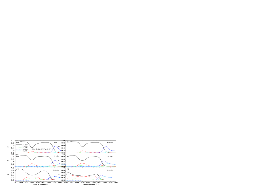
When the coupling of the SMM with the left electrode is stronger than that with the right electrode, i.e., , here we choose . Figures 1(a)-(c) show the average current, shot noise and skewness as a function of the bias voltage for , , , , , . Since the FCS for has the same bias-voltage-dependence as that for , which arises from the symmetry of the SMM Hamiltonian, we restrict our discussion to the case of . With increasing , the corresponding sequential tunneling threshold bias voltage has a tiny decrease and reach their minimums when increases to , see Fig. 1(a); but quantum noise obviously depends on the angle , see Fig. 1(b) and (c). The maximum peak of shot noise firstly increases and then decreases with increasing the angle from to . This characteristics of the shot noise can be understood with the help of the dynamic competition between effective fast and slow transport channelsWangSK ; Aghassi1 ; Safonov ; Djuric ; Aghassi2 ; Aguado . The molecular channel current is given byTimm ; Xue
| (16) | |||
| (17) |
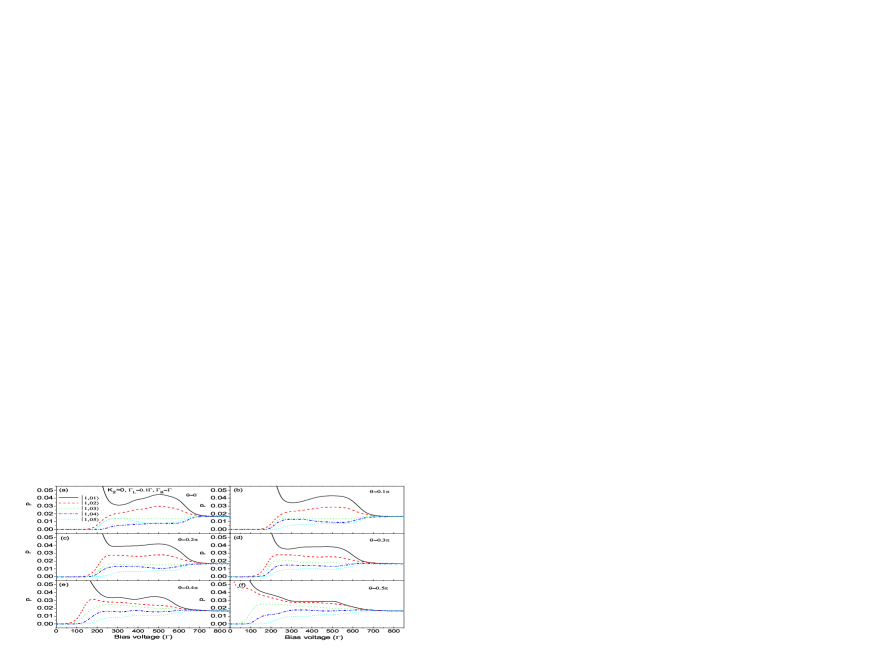
Here is a constant which related to the two molecular states but independent of the bias voltage, where (, , , , , for ) denote the eigenstates of the molecule with electrons tunneling into the molecule, which are arranged in an ascending order of their eigenvalues . is the occupied probability of the state . Since the maximum value of shot noise appears at a large bias voltage, the Fermi function changes very slowly with increasing bias voltage, i.e., . Thus the molecular channel currents are mainly determined by the probability distribution, and . In the presence of the transverse field and the transverse anisotropy, since the transitions between the molecular eigenstates are not restricted by the selection rule , the possible transport channels are , for example, there are a hundred transport channels for . Therefore, it is unpractical to give all the channel currents. In order to give a qualitative explanation for the effect of the angle on the shot noise, we plot the occupied probability of the five main molecular eigenstates as a function of bias voltage for , , , , , in Fig. 2. For the case of , the increase (or decrease) of the probability of the molecular eigenstate with high occupancy is always accompanied by the decrease (or increase) of the probability of the molecular eigenstates with the low occupancy. It is important that the active competition between the fast and slow transport channels depends on the angle . The competition between the probability of the five main molecular eigenstates for , and , as shown in Fig. 2, is stronger than that for and . Thus, the corresponding transport channel currents can form the so-called effective fast-and-slow transport channels, which leads to the maximum value of shot noise for , and are larger than that for and . In addition, it is interesting that some certain angles (e.g., , , ) may decrease the maximum super-Poissonian value of the skewness to sub-Poissonian value of although the angle (e.g., ) can also increase the maximum skewness value, see Fig. 1(c). In the simultaneity presence of the transverse field and the small transverse anisotropy, the active competition is further strengthened, so that the maximum shot noise value, which is sub-Poissonian value for , may be enhanced to super-Poissonian value for some certain angles, e.g., , and , see Fig. 1(e).
Compared to the case of , for the maximum shot noise and the skewness peaks are suppressed with increasing the angle . Fig. 3(a)-(c) show the average current, shot noise and skewness as a function of the bias voltage for , , , , , at . In this situation, the sequential tunneling threshold has the same characteristics as the case of . Apart from this feature, another important finding is that with increasing the angle from to , the maximum peaks of the shot noise and skewness can be reduced from super-Poissonian to sub-Poissonian value in the absence of the transverse anisotropy, see Fig. 3(b) and (c). Especially for the skewness, its super-Poissonian behavior seems more sensitive to the small than shot noise, see Fig. 3(c). The shot noise characteristics can also be understood in terms of the so-called fast and slow transport channels mechanism. Fig. 4 shows the occupancy probability of the five main singly-occupied molecular eigenstates as a function of bias voltage for various values of the angle, which determine corresponding transport channel currents. With increasing the angle from to , the competition between the probabilities of the eigenstates with high occupancy and the eigenstates with the low occupancy is gradually weakened, see Fig. 4. This means that the active competition between the fast-and-slow channel currents is gradually suppressed, thus leading to the maximum super-Poissonian value of shot noise is reduced even to sub-Poissonian value. Moreover, the small transverse anisotropy for also suppresses the maximum peaks of the shot noise and the skewness, and thus effaces the sensitivity of the maximum peaks of the shot noise and the skewness to the small , see Fig. 3(e) and (f).
IV CONCLUSIONS
We have studied the FCS of electron transport through a SMM with an arbitrary angle between the external magnetic field and the easy axis of the SMM above the sequential tunneling threshold. Since the presence of the transverse field and the transverse anisotropy leads to mixing of the spin eigenstates of , the spin selection rule for sequential tunneling processes are no longer applied to our model, as a result, there are transport channels participating in the electron transport. Therefore, the angle has a complex impact on the FCS. To facilitate the discussion of the origin of the shot noise, we put special emphasis on the dependence of the maximum noise on the angle of external magnetic field for strong asymmetric coupling to the two electrodes. For the case of , the maximum peak of the shot noise firstly increase and then decrease with increasing from to . In particular, the shot noise is further enhanced and even reaches super-Poissonian value when considering the small transverse anisotropy. For the case of , the maximum peaks of the shot noise and skewness can be reduced from super-Poissonian to sub-Poissonian value with increasing the angle from to . Especially for the skewness, its super-Poissonian behavior seems more sensitive to the small angle than shot noise, but this feature is suppressed when taking into account the small transverse anisotropy. These characteristics of shot noise can be understood as a result of the active competition between the fast and slow transport channels. The predictions regarding the high order current cumulants are very interesting for better understanding electron transport through individual single-molecule magnet, and the -dependence of the FCS can be helpful in understanding the experimental results because the angle is difficult to be controlled experimentally.
V ACKNOWLEDGMENTS
This work was supported by the Graduate Outstanding Innovation Item of Shanxi Province (Grant No. 20103001), the National Nature Science Foundation of China (Grant No. 10774094, No. 10775091, No. 10974124 and No. 11075099) and the Shanxi Nature Science Foundation of China (Grant No. 2009011001-1 and No. 2008011001-2).
References
- (1) H. B. Heersche, Z. de Groot, J. A. Folk, H. S. J. van der Zant, C. Romeike, M. R. Wegewijs, L. Zobbi, D. Barreca, E. Tondello, A. Cornia, Phys. Rev. Lett. 96, 206801 (2006).
- (2) Moon-Ho Jo, J. E. Grose, K. Baheti, M. M. Deshmukh, J. J. Sokol, E. M. Rumberger, D. N. Hendrickson, J. R. Long, H. Park, D. C. Ralph, Nano Lett. 6, 2014 (2006).
- (3) J. E. Grose, E. S. Tam, C. Timm, M. Scheloske, B. Ulgut, J. J. Parks, H. D. Abruna, W. Harneit, D. C. Ralph, Nature Mat. 7, 884 (2008).
- (4) A. S. Zyazin, J. W. G. van den Berg, E. A. Osorio, H. S. J. van der Zant, N. P. Konstantinidis, M. Leijnse, M. R. Wegewijs, F. May, W. Hofstetter, C. Danieli, and A. Cornia, Nano Lett. 10, 3307 (2010).
- (5) C. Romeike, M. R. Wegewijs, W. Hofstetter, H. Schoeller, Phys. Rev. Lett. 96, 196601 (2006); ibid. Phys. Rev. Lett. 97, 206601 (2006).
- (6) C. Romeike, M. R. Wegewijs, H. Schoeller, Phys. Rev. Lett. 96, 196805 (2006).
- (7) F. Elste, C. Timm, Phys. Rev. B 71, 155403 (2005); F. Elste, F. von Oppen, New J. Phys. 10, 065021 (2008); F. Elste, G. Weick, C. Timm, F. von Oppen, Appl. Phys. A 93, 345 (2008).
- (8) C. Timm, F. Elste, Phys. Rev. B 73, 235304 (2006); F. Elste, C. Timm, Phys. Rev. B 73, 235305 (2006); F. Elste, C. Timm, Phys. Rev. B 75, 195341 (2007); C. Timm, Phys. Rev. B 76, 014421 (2007).
- (9) Hai-Bin Xue, Y.-H. Nie, Z.-J. Li, J.-Q. Liang, J. Appl. Phys. 108, 033707 (2010).
- (10) Hai-Bin Xue, Y.-H. Nie, Z.-J. Li, J.-Q. Liang, Phys. Lett. A 375, 716 (2011).
- (11) M. N. Leuenberger, E. R. Mucciolo, Phys. Rev. Lett. 97, 126601 (2006); G. González, M. N. Leuenberger, Phys. Rev. Lett. 98, 256804 (2007); G. González, M. N. Leuenberger, E. R. Mucciolo, Phys. Rev. B 78, 054445 (2008).
- (12) M. Misiorny, J. Barnaś, Phys. Rev. B 75, 134425 (2007); ibid 76, 054448 (2007); ibid 77, 172414 (2008); M. Misiorny, J. Barnaś, Europhys. Lett. 78, 27003 (2007).
- (13) H.-Z. Lu, B. Zhou, and S.-Q. Shen, Phys. Rev. B 79, 174419 (2009).
- (14) B. Lapo, W. Wolfgang, Nature Mat. 7, 179 (2008).
- (15) M. J. Affronte, Mater. Chem. 19, 1731 (2009).
- (16) M. N. Leuenberger, D. Loss, Nature 410, 789 (2001).
- (17) J. Lehmann, A. Gaita-Ariño, E. Coronado and D. Loss, Nat. Nanotechnol. 2, 312 (2007).
- (18) D. Djukic, J. M. van Ruitenbeek, Nano Lett. 6, 789 (2006).
- (19) K.-I. Imura, Y. Utsumi, T. Martin, Phys. Rev. B 75, 205341 (2007).
- (20) S. Welack, J. B. Maddox, M. Esposito, U. Harbola, S. Mukamel, Nano Lett. 8, 1137 (2008).
- (21) B. Dong, H. Y. Fan, X. L. Lei, N. J. M. Horing, J. Appl. Phys. 105, 113702 (2009).
- (22) L. D. Contreras-Pulido and R. Aguado, Phys. Rev. B 81, 161309 (2010).
- (23) W. Belzig, Phys. Rev. B 71, 161301(R) (2005).
- (24) Ya. M. Blanter, M. Büttiker, Phys. Rep. 336, 1 (2000); Quantum Noise in Mesoscopic Physics, edited by Yu.V. Nazarov Kluwer, Dordrecht, 2003.
- (25) D. A. Bagrets, Yu. V. Nazarov, Phys. Rev. B 67, 085316 (2003).
- (26) X.-Q. Li, P. Cui, Y. J. Yan, Phys. Rev. Lett. 94, 066803 (2005).
- (27) X.-Q. Li, J. Luo, Y.-G. Yang, P. Cui, Y. J. Yan, Phys. Rev. B 71, 205304 (2005).
- (28) S.-K. Wang, H. Jiao, F. Li, X.-Q. Li, Y. J. Yan, Phys. Rev. B 76, 125416 (2007).
- (29) C. Timm, F. Elste, Phys. Rev. B 77, 195416 (2008).
- (30) W. H. Zurek, Phys. Rev. D 26, 1862 (1982).
- (31) C. Flindt, T. Novotný and A.-P. Jauho, Europhys. Lett. 69, 475 (2005); C. Flindt, T. Novotný, A. Braggio, M. Sassetti and A.-P. Jauho, Phys. Rev. Lett. 100, 150601 (2008); C. Flindt, T. Novotný, A. Braggio and A.-P. Jauho, Phys. Rev. B 82, 155407 (2010).
- (32) G. Kießlich, P. Samuelsson, A. Wacker, E. Schöll, Phys. Rev. B 73, 033312 (2006).
- (33) C. W. Groth, B. Michaelis, C. W. J. Beenakker, Phys. Rev. B 74, 125315 (2006).
- (34) J. Aghassi, A. Thielmann, M. H. Hettler, G. Schön, Phys. Rev. B 73, 195323 (2006).
- (35) A. Thielmann, M. H. Hettler, J. König, G. Schön, Phys. Rev. Lett. 95, 146806 (2005).
- (36) S. S. Safonov, A. K. Savchenko, D. A. Bagrets, O. N. Jouravlev, Yu. V. Nazarov, E. H. Linfield, D. A. Ritchie, Phys. Rev. Lett. 91, 136801 (2003).
- (37) I. Djuric, B. Dong, H. L. Cui, Appl. Phys. Lett. 87, 032105 (2005).
- (38) J. Aghassia, A. Thielmann, M. H. Hettler, G. Schön, Appl. Phys. Lett. 89, 052101 (2006).