Singular solutions of the $L^{2}$-supercritical biharmonic Nonlinear Schrödinger equation

Abstract

We use asymptotic analysis and numerical simulations to study peak-type singular solutions of the supercritical biharmonic NLS. These solutions have a quartic-root blowup rate, and collapse with a quasi self-similar universal profile, which is a zero-Hamiltonian solution of a fourth-order nonlinear eigenvalue problem.

1 Introduction

The focusing nonlinear Schrödinger equation (NLS)

$$i\psi_{t}(t,{\mathbf{x}})+\Delta\psi+\left|\psi\right|^{2\sigma}\psi=0,\qquad\psi(0,{\mathbf{x}})=\psi_{0}({\mathbf{x}})\in H^{1}({\mathbb{R}}^{d}),$$ (1)

where ${\mathbf{x}}=\left(x_{1},\dots,x_{d}\right)\in{\mathbb{R}}^{d}$ and $\Delta=\sum_{j=1}^{d}\partial_{j}^{2}$ is the Laplacian, has been the subject of intense study, due to its role in various areas of physics, such as nonlinear optics and Bose-Einstein Condensates (BEC). It is well-known that the NLS (1) possesses solutions that become singular in a finite time [SS99].

In recent years, there has been a growing interest in extending NLS theory to the focusing biharmonic nonlinear Schrödinger equation (BNLS)

$$i\psi_{t}(t,{\mathbf{x}})-\Delta^{2}\psi+\left|\psi\right|^{2\sigma}\psi=0,\qquad\psi(0,{\mathbf{x}})=\psi_{0}({\mathbf{x}})\in H^{2}({\mathbb{R}}^{d}),$$ (2)

where $\Delta^{2}$ is the biharmonic operator. The BNLS (2) is called “$L^{2}$-critical”, or simply “critical” if $\sigma d=4$. In this case, equation (2) can be rewritten as

$$i\psi_{t}(t,{\mathbf{x}})-\Delta^{2}\psi+\left|\psi\right|^{8/d}\psi=0,\qquad\psi(0,{\mathbf{x}})=\psi_{0}({\mathbf{x}})\in H^{2}({\mathbb{R}}^{d}).$$ (3)

Correspondingly, the BNLS with $0<\sigma d<4$ is called subcritical, and the BNLS with $\sigma d>4$ is called supercritical. This is analogous to the NLS, where the critical case is $\sigma d=2$.

BNLS solutions preserve the power ($L^{2}$ norm)

$$P(t)\equiv P(0),\qquad P=||\psi||_{2}^{2},$$

and the Hamiltonian

$$H(t)\equiv H(0),\qquad H=||\Delta\psi||_{2}^{2}-\frac{1}{\sigma+1}||\Delta\psi||_{2\sigma+2}^{2\sigma+2}.$$

In [BAKS00], Ben-Artzi, Koch and Saut proved that when $\sigma$ is in the $H^{2}$-subcritical regime

$$\begin{cases}0<\sigma&\quad d\leq 4,\\ 0<\sigma<\frac{4}{d-4}&\quad d>4,\end{cases}$$ (4)

the BNLS (2) is locally well-posed in $H^{2}$. Global existence and scattering of BNLS solutions in the $H^{2}$-critical case $\sigma=4/(d-4)$ were studied by Miao, Xu and Zhao [MXZ09] and by Pausader [Pau09b]. The latter work also showed well-posedness for small data. The $H^{2}$-critical defocusing BNLS was studied by Miao, Xu and Zhao [MXZ08] and by Pausader [Pau07, Pau09a].

The above studies focused on non-singular solutions. In this work, we study singular solutions of the BNLS in $H^{2}$, i.e., solutions that exist in $H^{2}({\mathbb{R}}^{d})$ over some finite time interval $t\in[0,{T_{\rm c}})$, but for which $\displaystyle\lim_{t\to{T_{\rm c}}}{\left\|{\psi}\right\|}_{H^{2}}=\infty.$ The first study of singular BNLS solutions was done by Fibich, Ilan and Papanicolau [FIP02], who proved the following results:

Theorem 1.

Let $\psi_{0}\in H^{2}$. Then, the solution of the subcritical BNLS (2) exists globally in $H^{2}$.

Theorem 2.

Let $\psi_{0}\in H^{2}$, and let ${\left\|{\psi_{0}}\right\|}_{2}^{2}<{P_{\text{cr}}^{\text{\tiny B}}}$, where ${P_{\text{cr}}^{\text{\tiny B}}}={\left\|{{R_{\text{\tiny B}}}}\right\|}_{2}^{2}$, and ${R_{\text{\tiny B}}}$ is the ground state of

$$-\Delta^{2}{R_{\text{\tiny B}}}({\mathbf{x}})-{R_{\text{\tiny B}}}+|{R_{\text{\tiny B}}}|^{8/d}{R_{\text{\tiny B}}}=0.$$ (5)

Then, the solution of the critical BNLS (3) exists globally in $H^{2}$.

The simulations in [FIP02] suggested that there exist singular solutions for $\sigma d=4$ and $\sigma d>4$, and that these singularities are of the blowup type, namely, the solution becomes infinitely localized. However, in contradistinction with NLS theory, there is currently no rigorous proof that solutions of the BNLS can become singular in either the critical or the supercritical case.

Most subsequent research of singular BNLS solutions focused on the critical case. Chae, Hong and Lee [CHL11], showed that radial singular solutions of (3) have a power-concentration property. In [BFM10b], we showed that radial singular solutions are quasi self-similar. We also proved, without assuming radial symmetry, that the blowup rate is bound by a quartic-root, the power-concentration property and the existence of the ground-state of (5). The two latter properties were also proved by Zhu, Zhang and Yang [ZZY10]. In [BFM10b], we also provided informal analysis and numerical evidence that peak-type singular solutions of the critical BNLS collapse with a quasi self-similar ${R_{\text{\tiny B}}}$ profile at a blowup rate which is slightly faster than the quartic-root bound.

In this work, we use asymptotic analysis and numerics to find and characterize peak-type singular solutions of the supercritical BNLS. We find that their properties mirror those of the supercritical NLS. Ring-type singular solutions of the supercritical BNLS were studied in [BFG10, BFM10a].

1.1 Summary of results

We analyze singular solutions of the focusing $L^{2}$-supercritical and $H^{2}$-subcritical BNLS, i.e., when

$$\begin{cases}4/d<\sigma&d\leq 4,\\ 4/d<\sigma<\frac{4}{d-4}&d>4.\end{cases}$$ (6)

We assume radial symmetry, i.e., that $\psi=\psi(t,r)$, where $r=|{{\mathbf{x}}}|$. In this case, equation (2) reduces to

$$i\psi_{t}(t,r)-\Delta^{2}_{r}\psi+\left|\psi\right|^{2\sigma}\psi=0,\qquad\psi(0,r)=\psi_{0}(r),$$ (7)

where

$$\Delta_{r}^{2}=\partial_{r}^{4}+\frac{2(d-1)}{r}\partial_{r}^{3}+\frac{(d-1)(d-3)}{r^{2}}\partial_{r}^{2}-\frac{(d-1)(d-3)}{r^{3}}\partial_{r}$$

is the radial biharmonic operator.

The paper is organized as follows. In Section 2, we show that the supercritical BNLS admits the explicit self-similar singular solutions

$$\psi_{S_{\text{\tiny B}}}(t,r)=\frac{1}{L^{2/\sigma}(t)}{S_{\text{\tiny B}}}\left(\frac{r}{L(t)}\right)e^{i\nu\int\frac{1}{L^{4}(t^{\prime})}dt^{\prime}},$$ (8)

where the blowup rate of $L(t)$ is exactly a quartic-root

$$L(t)=\kappa({T_{\rm c}}-t)^{1/4},\qquad\kappa>0,$$

and the self-similar profile ${S_{\text{\tiny B}}}(\rho)$ is a solution of

$$\begin{gathered}-\nu{S_{\text{\tiny B}}}(\rho)+i\frac{\kappa^{4}}{4}\left(\frac{2}{\sigma}{S_{\text{\tiny B}}}+\rho{S_{\text{\tiny B}}}^{\prime}\right)-\Delta_{\rho}^{2}{S_{\text{\tiny B}}}+{\left|{{S_{\text{\tiny B}}}}\right|}^{2\sigma}{S_{\text{\tiny B}}}=0,\\ {S_{\text{\tiny B}}}^{\prime}(0)={S_{\text{\tiny B}}}^{\prime\prime\prime}(0)=0,\qquad{S_{\text{\tiny B}}}(\infty)=0.\end{gathered}$$ (9)

WKB analysis of the large-$\rho$ behavior of ${S_{\text{\tiny B}}}$ shows that it belongs to $L^{2+2\sigma}$, but not to $L^{2}$. Since $\lim_{t\to{T_{\rm c}}}{\left\|{\psi_{S_{\text{\tiny B}}}}\right\|}_{2+2\sigma}=\infty$, $\psi_{S_{\text{\tiny B}}}$ is a singular solution in $L^{2+2\sigma}$, but not in $H^{2}$. To the best of our knowledge, this is the first time that explicit singular solutions of the BNLS are presented.

In Section 2.1 we show that the zero-Hamiltonian solutions of (9) satisfy the boundary condition

$$\lim_{\rho\to\infty}\left(\rho S^{\prime}+\left(\frac{2}{\sigma}+i\frac{4\nu}{\kappa^{4}}\right)S\right)\rho^{\gamma}=0,\qquad\frac{2}{3}\left(d-2-\frac{2}{\sigma}\right)<\gamma<4+\frac{2}{\sigma}.$$

In analogy with the supercritical NLS, we conjecture that for any $d$, $\sigma$ and $\nu$, there is unique admissible solution ${S_{\text{\tiny B}}}^{\rm admis.}(\rho)$, which has a zero Hamiltonian and is monotonically decreasing. This solution is attained for a unique $\kappa=\kappa^{\rm admis.}(\sigma,d,\nu)>0$. While a rigorous existence proof for the ${S_{\text{\tiny B}}}$ profile remains open, we provide numerical support for the existence of the admissible solutions.

In Section 3 we consider $H^{2}$ singular solutions. Using informal asymptotic analysis and the analogy with the supercritical NLS, we conjecture that these solutions undergo a quasi self-similar collapse with the $\psi_{S_{\text{\tiny B}}}$ profile, where ${S_{\text{\tiny B}}}$ is the unique admissible solution ${S_{\text{\tiny B}}}^{\rm admis.}$. The blowup rate of these solutions is given by $L(t)\sim\kappa^{\rm admis.}({T_{\rm c}}-t)^{1/4}$. These characteristics are confirmed numerically, in simulations of both the one-dimensional and the two-dimensional BNLS.

The numerical simulations of the BNLS were performed using the IGR/SGR method [RW00, DG09], see [BFM10a] for further details. The numerical solution of the nonlinear fourth-order ODE for ${S_{\text{\tiny B}}}$ is obtained using a modified Petviashvili (SLSR) method, which is described in the appendix. The code is available online at http://www.math.tau.ac.il/$\sim$fibich/publications.html

The results of this study are based on asymptotic analysis and numerical simulations, but not on rigorous analysis. These results show that there is a striking analogy between collapse of peak type solutions in the supercritical NLS and the supercritical BNLS. We note that the rigorous theory for singular solutions of the supercritical NLS is much less developed than that for the critical NLS. Indeed, a rigorous proof of the blowup rate and blowup profile of the supercritical NLS was obtained very recently, and only in the slightly-supercritical regime $0<\sigma d-2\ll 1$ [MRS09]. We hope that this study will motivate a similar rigorous treatment of the supercritical BNLS.

2 Explicit singular solutions

Let us look for explicit self-similar solutions of the supercritical BNLS (2). Since the BNLS is invariant under the dilation symmetry $r\mapsto\frac{r}{L},t\mapsto\frac{t}{L^{4}},\psi\mapsto\frac{1}{L^{2/\sigma}}\psi$, where $L$ is a constant, this suggests a self-similar solution of the form

$$\psi_{S_{\text{\tiny B}}}(t,r)=\frac{1}{L^{2/\sigma}(t)}{S_{\text{\tiny B}}}\left(\rho\right)e^{i\tau(t)},\qquad\rho=\frac{r}{L(t)}.$$ (10)

Substituting $\psi_{S_{\text{\tiny B}}}$ in the BNLS gives

$$-\tau^{\prime}(t)L^{4}(t){S_{\text{\tiny B}}}(\rho)-iL^{3}(t)L_{t}\left(\frac{2}{\sigma}{S_{\text{\tiny B}}}+\rho{S_{\text{\tiny B}}}^{\prime}\right)-\Delta_{\rho}^{2}{S_{\text{\tiny B}}}+{\left|{{S_{\text{\tiny B}}}}\right|}^{2\sigma}{S_{\text{\tiny B}}}=0.$$ (11)

Since ${S_{\text{\tiny B}}}$ is only a function of $\rho$, equation (11) must be independent of $t$. Therefore, there exists a real constant $\kappa$ such that

$$L^{3}L_{t}\equiv\frac{1}{4}\left(L^{4}\right)_{t}\equiv-\kappa^{4}/4.$$

Hence, $L(t)$ is a quartic root, i.e.,

$$L(t)=\kappa\sqrt[4]{{T_{\rm c}}-t},\qquad\kappa>0.$$ (12)

Likewise, since ${S_{\text{\tiny B}}}$ is only a function of $\rho$, then $\tau^{\prime}(t)L^{4}(t)\equiv\nu$. Hence,

$$\tau(t)=\nu\int_{s=0}^{t}\frac{1}{L^{4}(s)}ds=-\frac{\nu}{\kappa^{4}}\ln\left(1-\frac{t}{{T_{\rm c}}}\right).$$ (13)

Substituting (12) and (13) in (11) shows that the equation for ${S_{\text{\tiny B}}}$ is

$$-\nu{S_{\text{\tiny B}}}(\rho)+i\frac{\kappa^{4}}{4}\left(\frac{2}{\sigma}{S_{\text{\tiny B}}}+\rho{S_{\text{\tiny B}}}^{\prime}\right)-\Delta_{\rho}^{2}{S_{\text{\tiny B}}}+{\left|{{S_{\text{\tiny B}}}}\right|}^{2\sigma}{S_{\text{\tiny B}}}=0.$$ (14a)

Since $${S_{\text{\tiny B}}}$$ is radially-symmetric and decays at infinity, it should satisfy the boundary conditions

$${S_{\text{\tiny B}}}^{\prime}(0)={S_{\text{\tiny B}}}^{\prime\prime\prime}(0)=0,\qquad{S_{\text{\tiny B}}}(\infty)=0.$$ (14b)

Equation (14) has the two parameters $\nu$ and $\kappa$. Note, however, that

$${S_{\text{\tiny B}}}(\rho;\kappa,\nu):=\nu^{\frac{1}{2\sigma}}\tilde{{S_{\text{\tiny B}}}}(\nu^{1/4}\rho;\tilde{\kappa}=\kappa/\nu^{1/4}),$$ (15)

where $\tilde{{S_{\text{\tiny B}}}}(\rho;\tilde{\kappa})$ is the solution of (14) with $\nu=1$, i.e.,

$$-\tilde{{S_{\text{\tiny B}}}}(\rho)+i\frac{\kappa^{4}}{4}\left(\frac{2}{\sigma}\tilde{{S_{\text{\tiny B}}}}+\rho\tilde{{S_{\text{\tiny B}}}}^{\prime}\right)-\Delta_{\rho}^{2}\tilde{{S_{\text{\tiny B}}}}+{\left|{\tilde{{S_{\text{\tiny B}}}}}\right|}^{2\sigma}\tilde{{S_{\text{\tiny B}}}}=0.$$ (16a)

subject to

$$\tilde{{S_{\text{\tiny B}}}}^{\prime}(0)=\tilde{{S_{\text{\tiny B}}}}^{\prime\prime\prime}(0)=0,\qquad\tilde{{S_{\text{\tiny B}}}}(\infty)=0.$$ (16b)

Equation (16) can be viewed as a nonlinear eigenvalue problem with the eigenvalue $\kappa$ and eigenfunction ${S_{\text{\tiny B}}}$. By analogy with the supercritical NLS [KL95, Bud01], we make the following conjecture:

Conjecture 3.

Let $\sigma$ be in the $L^{2}$ supercritical and $H^{2}$-subcritical regime (6). Then, there exists a solution $\left\{\tilde{{S_{\text{\tiny B}}}}(\rho),\tilde{\kappa}\right\}$ to equation (16), such that $\tilde{{S_{\text{\tiny B}}}}\not\equiv 0$ and $\tilde{\kappa}>0$.

Hence, we have the following result:

Lemma 4.

Assume that Conjecture 3 holds, and let ${S_{\text{\tiny B}}}(\rho;\kappa,\nu)$ be a nontrivial solution of (14). Then,

$$\psi_{S_{\text{\tiny B}}}(t,r)=\frac{1}{L^{2/\sigma}(t)}{S_{\text{\tiny B}}}\left(\frac{r}{L(t)}\right)e^{i\nu\int^{t}\frac{1}{L^{4}(s)}ds},\qquad L(t)=\kappa\sqrt[4]{{T_{\rm c}}-t},$$ (17)

is an explicit solution of the BNLS equation (2).

As $\rho\to\infty$, the nonlinear term in (14) becomes negligible, and (14a) reduces to

$$-\nu{S_{\text{\tiny B}}^{lin}}(\rho)-\Delta_{\rho}{S_{\text{\tiny B}}^{lin}}+i\frac{\kappa^{4}}{4}\left(\frac{2}{\sigma}{S_{\text{\tiny B}}^{lin}}+\rho({S_{\text{\tiny B}}^{lin}})_{\rho}\right)=0,$$ (18)

where

$$\Delta_{\rho}^{2}=-\frac{(d-1)(d-3)}{\rho^{3}}\partial_{\rho}+\frac{(d-1)(d-3)}{\rho^{2}}\partial_{\rho}^{2}+\frac{2(d-1)}{\rho}\partial_{\rho}^{3}+\partial_{\rho}^{4}~{}.$$

We now use WKB to find the large $\rho$ behavior of (18):

Lemma 5.

Let ${S_{\text{\tiny B}}^{lin}}(\rho)$ be a solution of (18). Then,

$${S_{\text{\tiny B}}^{lin}}\sim c_{1}{S_{\text{\tiny B}}}_{,1}(\rho)+c_{2}{S_{\text{\tiny B}}}_{,2}(\rho)+c_{3}{S_{\text{\tiny B}}}_{,3}(\rho)+c_{4}{S_{\text{\tiny B}}}_{,4}(\rho),\qquad\rho\to\infty,$$

where $\left\{c_{i}\right\}_{i=1}^{4}$ are complex constants,

$${S_{\text{\tiny B}}}_{,1}(\rho) \sim \rho^{-\frac{2}{\sigma}-i\frac{4\nu}{\kappa^{4}}},$$

$${S_{\text{\tiny B}}}_{,2}(\rho) \sim \frac{1}{\rho^{\frac{2}{3\sigma}(\sigma d-1)}}\exp\left(-i{\frac{3}{4\sqrt[3]{4}}}(\kappa\rho)^{4/3}+i\frac{4\nu}{3\kappa^{4}}\log(\rho)\right),$$

$${S_{\text{\tiny B}}}_{,3}(\rho) \sim \frac{\exp\left(+~{}\frac{3\sqrt{3}}{8\sqrt[3]{4}}(\kappa\rho)^{4/3}\right)}{\rho^{\frac{2}{3\sigma}(\sigma d-1)}}\exp\left(+i\frac{3\sqrt{3}}{8\sqrt[3]{4}}(\kappa\rho)^{4/3}+i\frac{4\nu}{3\kappa^{4}}\log(\rho)\right),$$

$${S_{\text{\tiny B}}}_{,4}(\rho) \sim \frac{\exp\left(-~{}\frac{3\sqrt{3}}{8\sqrt[3]{4}}(\kappa\rho)^{4/3}\right)}{\rho^{\frac{2}{3\sigma}(\sigma d-1)}}\exp\left(+i\frac{3\sqrt{3}}{8\sqrt[3]{4}}(\kappa\rho)^{4/3}+i\frac{4\nu}{3\kappa^{4}}\log(\rho)\right).$$

Proof.

In order to apply the WKB method, we substitute ${S_{\text{\tiny B}}^{lin}}(\rho)=\exp(w(\rho))$, and expand

$$w(\rho)\sim w_{0}(\rho)+w_{1}(\rho)+\dots\;.$$

Substituting $w_{0}(\rho)=\alpha\rho^{p}$ and balancing terms shows that $p=4/3$, and that the equation for the leading-order, the $\mathcal{O}\left(\rho^{4/3}\right)$ terms, is

$$\left(w_{0}^{\prime}\right)^{3}=\left(\frac{4\alpha}{3}\right)^{3}\rho=i\frac{\kappa^{4}}{4}\rho.$$

Therefore,

$$\alpha=\frac{3}{4}\sqrt[3]{i\frac{\kappa^{4}}{4}}=\frac{3\kappa^{4/3}}{4\sqrt[3]{4}}\cdot\left\{-i,\frac{\sqrt{3}+i}{2},\frac{-\sqrt{3}+i}{2}\right\}.$$

The equation for the next order, the $\mathcal{O}\left(1\right)$ terms, is

$$\nu+i\frac{\kappa^{4}}{2}d=i\frac{\kappa^{4}}{4}\left(\frac{2}{\sigma}+3\rho w_{1}^{\prime}\right),$$

implying that

$$w_{1}=\frac{1}{3}\left(\frac{2}{\sigma}(1-\sigma d)+\frac{4\nu}{\kappa^{4}}i\right)\log\rho.$$

The next-order terms are $\mathcal{O}\left(\rho^{-4/3}\right)=o(1)$ and can be neglected. We therefore obtain the three solutions ${S_{\text{\tiny B}}}_{,2}$, ${S_{\text{\tiny B}}}_{,3}$, and ${S_{\text{\tiny B}}}_{,4}$.

Since (18) is a fourth order ODE, another solution is required. To obtain the fourth solution, we substitute $w_{0}\sim\beta\log(\rho)$ in (18) and obtain that the equation for the leading-order, the $\mathcal{O}(1)$ terms, is

$$-\nu+i\frac{\kappa^{4}}{4}\left(\frac{2}{\sigma}+\beta\right)=0,$$

and that the next-order terms are $\mathcal{O}\left(\rho^{-4}\right)=o(1)$ and can be neglected. The fourth solution is therefore ${S_{\text{\tiny B}}}_{,1}$.

∎

Equation (18) thus has the two algebraically-decaying solutions, ${S_{\text{\tiny B}}}_{,1}$ and ${S_{\text{\tiny B}}}_{,2}$, the exponentially-increasing solution ${S_{\text{\tiny B}}}_{,3}$, and the exponentially-decreasing solution ${S_{\text{\tiny B}}}_{,4}$. The fact that ${S_{\text{\tiny B}}}_{,3}$ increases exponentially as $\rho\to\infty$ is inconsistent with the boundary condition (14b). Therefore,

$${S_{\text{\tiny B}}}(\rho)\sim c_{1}{S_{\text{\tiny B}}}_{,1}(\rho)+c_{2}{S_{\text{\tiny B}}}_{,2}(\rho)+c_{4}{S_{\text{\tiny B}}}_{,4}(\rho).$$ (19)

Since $\sigma d>4$, the exponent $\frac{2}{3\sigma}(\sigma d-1)$ of ${S_{\text{\tiny B}}}_{,2}$ is larger that the exponent $\frac{2}{\sigma}$ of ${S_{\text{\tiny B}}}_{,1}$, hence

$${S_{\text{\tiny B}}}_{,1}\gg{S_{\text{\tiny B}}}_{,2},\qquad\rho\to\infty.$$ (20)

.

Direct calculations give that

$${S_{\text{\tiny B}}}_{,1}\not\in L^{2}({\mathbb{R}}^{d}), \Delta{S_{\text{\tiny B}}}_{,1}\in L^{2}({\mathbb{R}}^{d}), {S_{\text{\tiny B}}}_{,1}\in L^{2+2\sigma}({\mathbb{R}}^{d}),$$ (21a)

$${S_{\text{\tiny B}}}_{,2}\in L^{2}({\mathbb{R}}^{d}), \Delta{S_{\text{\tiny B}}}_{,2}\not\in L^{2}({\mathbb{R}}^{d}), {S_{\text{\tiny B}}}_{,2}\in L^{2+2\sigma}({\mathbb{R}}^{d}),$$ (21b)

$${S_{\text{\tiny B}}}_{,4}\in L^{2}({\mathbb{R}}^{d}), \Delta{S_{\text{\tiny B}}}_{,4}\in L^{2}({\mathbb{R}}^{d}), {S_{\text{\tiny B}}}_{,4}\in L^{2+2\sigma}({\mathbb{R}}^{d}).$$ (21c)

Therefore, ${S_{\text{\tiny B}}}$ is in $L^{2+2\sigma}$. Unless $c_{1}=c_{2}=0$, however, ${S_{\text{\tiny B}}}$ is not in $H^{2}$. Furthermore, since

$${\left\|{\psi_{{S_{\text{\tiny B}}}}}\right\|}_{2+2\sigma}^{2+2\sigma}=\frac{1}{L^{4/\sigma-(d-4)}(t)}{\left\|{{S_{\text{\tiny B}}}}\right\|}_{2+2\sigma}^{2+2\sigma},$$

then $\psi_{S_{\text{\tiny B}}}\in L^{2+2\sigma}$ for $0\leq t<{T_{\rm c}}$. In the $H^{2}$-subcritical regime $4/\sigma-(d-4)>0$. Therefore,

$$\lim_{t\to{T_{\rm c}}}{\left\|{\psi_{S_{\text{\tiny B}}}}\right\|}_{2+2\sigma}=\infty.$$

Hence,

Lemma 6.

Assume that Conjecture 3 holds. Then, $\psi_{S_{\text{\tiny B}}}$ is an explicit solution of the BNLS equation (2) that becomes singular in $L^{2+2\sigma}$ as $t\to{T_{\rm c}}$.

2.1 Zero-Hamiltonian solutions

As is the case of peak-type solutions of the supercritical NLS, a key role is played by the zero-Hamiltonian solutions.

Theorem 7.

Let $\sigma$ be in the $L^{2}$ supercritical and $H^{2}$-subcritical regime (6). Let ${S_{\text{\tiny B}}}$ be a solution of (14). If $H\left[{S_{\text{\tiny B}}}\right]<\infty$, then $H\left[{S_{\text{\tiny B}}}\right]=0$.

Proof.

The Hamiltonian of $\psi_{S_{\text{\tiny B}}}$, see (17), is equal to

$$H\left[\psi_{S_{\text{\tiny B}}}\right]=\frac{1}{L^{4/\sigma-(d-4)}}H\left[{S_{\text{\tiny B}}}\right].$$

From $H^{2}$-subcriticality, it follows that $L^{-4/\sigma-4+d}(t)\neq{\it const}$. Therefore, Hamiltonian conservation ($H\left[\psi_{S_{\text{\tiny B}}}\right]\equiv{\it const}$) implies that $H\left[{S_{\text{\tiny B}}}\right]=0$. ∎

Lemma 8.

Let $\sigma$ be in the $L^{2}$ supercritical and $H^{2}$-subcritical regime (6). Let ${S_{\text{\tiny B}}}(\rho)$ be a zero-Hamiltonian solution of (14). Then,

1. $c_{2}=c_{3}=0$.

2. If $c_{1}\neq 0$ then

   $${S_{\text{\tiny B}}}(\rho)\sim c_{1}{S_{\text{\tiny B}}}_{,1}(\rho),\qquad\rho\to\infty,$$ (22)

   or, equivalently,

   $$\lim_{\rho\to\infty}\left(\rho S^{\prime}+\left(\frac{2}{\sigma}+i\frac{4\nu}{\kappa^{4}}\right)S\right)\rho^{\gamma}=0,$$ (23a)

   where

   $$\gamma_{0}<\gamma<\gamma_{1},\qquad\gamma_{0}=\frac{2}{3}\left(d-2-\frac{2}{\sigma}\right),\quad\gamma_{1}=4+\frac{2}{\sigma}.$$ (23b)

   Moreover, $${S_{\text{\tiny B}}}\in L^{2\sigma+2} {S_{\text{\tiny B}}}\not\in L^{2}$$ and .

Proof.

The exponentially increasing solution $c_{3}{S_{\text{\tiny B}}}_{,3}$ must vanish, as explained above. Convergence of the Hamiltonian requires that $\Delta{S_{\text{\tiny B}}}\in L^{2}$. Since $\Delta{S_{\text{\tiny B}}}_{,2}\not\in L^{2}$, see (21), it follows that $c_{2}=0$. Since ${S_{\text{\tiny B}}}_{,1}\not\in L^{2}$, then ${S_{\text{\tiny B}}}\not\in L^{2}$.

To show that (23) is equivalent to demanding that $c_{2}=0$, we first note that in the $H^{2}$-subcritical regime $d-4<\frac{4}{\sigma}$ and so $\gamma_{0}<\frac{2}{3}\left(2+\frac{2}{\sigma}\right)<\gamma_{1}$. Next, direct calculation gives that

$$\left(\rho\frac{d}{d\rho}+\frac{2}{\sigma}+i\frac{4\nu}{\kappa^{4}}\right){S_{\text{\tiny B}}}_{,2}\sim{\cal O}\left(\rho^{4/3-\frac{2}{3\sigma}(\sigma d-1)}\right),\quad\rho\to\infty,$$

and that

$$\left(\rho\frac{d}{d\rho}+\frac{2}{\sigma}+i\frac{4\nu}{\kappa^{4}}\right){S_{\text{\tiny B}}}_{,1}\sim{\cal O}\left(\rho^{-\frac{2}{\sigma}-4}\right),\quad\rho\to\infty,$$

where the LHS is the result of the next term in the WKB approximation of ${S_{\text{\tiny B}}}_{,1}$. Therefore,

$$\rho^{\gamma}\left(\rho\frac{d}{d\rho}+\frac{2}{\sigma}+i\frac{4\nu}{\kappa^{4}}\right){S_{\text{\tiny B}}}\sim{\cal O}\left(c_{1}\cdot\rho^{\gamma-\frac{2}{\sigma}-4}\right)+{\cal O}\left(c_{2}\cdot\rho^{\gamma+4/3-\frac{2}{3\sigma}(\sigma d-1)}\right),\quad\rho\to\infty.$$

Since, for $\gamma_{0}<\gamma<\gamma_{1}$,

$$\lim_{\rho\to\infty}\rho^{\gamma-\frac{2}{\sigma}-4}=0,\qquad\lim_{\rho\to\infty}\rho^{\gamma+\frac{4}{3}-\frac{2}{3\sigma}(\sigma d-1)}=\infty,$$

it follows that $c_{2}=0$ if and only if the limit (23a) is satisfied. ∎

The fourth-order nonlinear ODE (14a) requires four boundary conditions. Three boundary conditions are given by (14b), and the fourth condition will be the zero-Hamiltonian condition (23a). Generically, one can expect that for a given $\nu$, this nonlinear eigenvalue problem has an enumerable number of eigenvalues $\kappa^{(n)}$ with corresponding eigenfunctions ${S_{\text{\tiny B}}}^{(n)}$. As in the case of the supercritical NLS [KL95, Bud01], we conjecture that for any $(\sigma,d,\nu)$ there is a unique admissible solution, which is monotonically decreasing.

Conjecture 9.

Let $\sigma$ be in the $L^{2}$ supercritical and $H^{2}$-subcritical regime (6), and let $\nu>0$. Then, the nonlinear eigenvalue problem posed by equation (14a), subject to the boundary conditions

$${S_{\text{\tiny B}}}^{\prime}(0)={S_{\text{\tiny B}}}^{\prime\prime\prime}(0)={S_{\text{\tiny B}}}(\infty)=0,\qquad\lim_{\rho\to\infty}\left(\rho S^{\prime}+\left(\frac{2}{\sigma}+i\frac{4\nu}{\kappa^{4}}\right)S\right)\rho^{\gamma}=0,$$ (24)

where $\gamma$ satisfies (23b), admits a unique eigenpair $({S_{\text{\tiny B}}}^{\rm admis.}(\rho),\kappa^{\rm admis.})$, such that

$$\kappa^{\rm admis.}=\kappa^{\rm admis.}(\sigma,d,\nu)>0,$$

and $|{S_{\text{\tiny B}}}^{\rm admis.}(\rho)|$ is monotonically-decreasing. Furthermore,

$${S_{\text{\tiny B}}}^{\rm admis.}(\rho)\sim c\rho^{-2/\sigma-4\nu i/\kappa^{4}},\qquad\rho\longrightarrow\infty,$$

and

$$\kappa^{\rm admis.}(\sigma,d,\nu)=\nu^{1/4}\tilde{\kappa}^{\rm admis.}(\sigma,d),\qquad\tilde{\kappa}^{\rm admis.}:=\kappa^{\rm admis.}(\sigma,d,\nu=1).$$

3 Peak-type $H^{2}$-singular solutions

3.1 Informal analysis

As in the supercritical NLS  [LPSS88, SKL93], we expect that singular peak-type solutions of the supercritical BNLS undergo a quasi self-similar collapse, so that

$$\psi(t,r)\sim\begin{cases}\psi_{S_{\text{\tiny B}}}(t,r)&0\leq r\leq r_{c},\\ \psi_{\text{non-singular}}(t,r)\quad&r\geq r_{c},\end{cases}$$ (25)

where $\psi_{S_{\text{\tiny B}}}$ is the self-similar profile (10). The singular region $r\in[0,r_{c}]$ is constant in the coordinate $r$. Therefore, in the rescaled variable $\rho=r/L(t)$, the singular region $\rho\in[0,r_{c}/L(t)]$ becomes infinite as $L(t)\to 0$. This is in contradistinction with the critical-BNLS case, where the singular region $\rho\in[0,\rho_{c}]$ is constant in the rescaled variable $\rho$, but shrinks to a point in the original coordinate $r$ [BFM10b].

Lemma 10.

Let $\sigma d>4$, and let $\psi$ be a peak-type singular solution of the BNLS that collapses with the $\psi_{S_{\text{\tiny B}}}$ profile (10). If $L(t)\sim\kappa({T_{\rm c}}-t)^{p}$, then $p\geq\frac{1}{4}$. Furthermore,

• If $p=1/4$ if then the self-similar profile ${S_{\text{\tiny B}}}(\rho)$ satisfies the equation (14a).

• If $p>1/4$, then the profile satisfies the equation

  $$-\Delta^{2}{R_{\text{\tiny B}}}({\mathbf{x}})-{R_{\text{\tiny B}}}+|{R_{\text{\tiny B}}}|^{2\sigma}{R_{\text{\tiny B}}}=0.$$ (26)

Proof.

If $\psi\sim\psi_{S_{\text{\tiny B}}}$, then the equation for ${S_{\text{\tiny B}}}$ is

$$-\nu{S_{\text{\tiny B}}}-i\left(\lim_{t\to{T_{\rm c}}}L_{t}L^{3}\right)\left(\frac{2}{\sigma}{S_{\text{\tiny B}}}+\rho{S_{\text{\tiny B}}}^{\prime}\right)-\Delta^{2}_{\rho}{S_{\text{\tiny B}}}+{\left|{{S_{\text{\tiny B}}}}\right|}^{2\sigma}{S_{\text{\tiny B}}}=0,$$ (27)

implying that $L_{t}L^{3}$ should be bounded as $t\to{T_{\rm c}}$. Since $L^{3}L_{t}\sim-p\kappa^{4}({T_{\rm c}}-t)^{4p-1}$, it follows that $p\geq\frac{1}{4}$. If $p=1/4$, then equation (27) reduces to (14a), see Section 2. ∎

From Hamiltonian conservation it follows that $H\left[\psi_{S_{\text{\tiny B}}}\right]$ is bounded, because otherwise the non-singular region would also have an infinite Hamiltonian. Therefore, from Theorem 7 it follows that $H\left[{S_{\text{\tiny B}}}\right]=0$.

In Lemma 8 we saw that the zero-Hamiltonian solutions of (14a) are in $L^{2+2\sigma}$, but not in $L^{2}$. Hence, $\psi_{S_{\text{\tiny B}}}\not\in L^{2}$. From power conservation, however, it follows that if $\psi_{0}\in H^{2}$, then $\psi\in L^{2}$. As in the NLS case, see [BP92], this “contradiction” can be resolved as follows.

Corollary 11.

Let ${S_{\text{\tiny B}}}(\rho)$ be a zero-Hamiltonian solution of (14). Then, ${\left\|{{S_{\text{\tiny B}}}}\right\|}_{2}=\infty$. Nevertheless, $\displaystyle\lim_{t\to{T_{\rm c}}}{\left\|{\psi_{S_{\text{\tiny B}}}}\right\|}_{L^{2}(r<r_{c})}<\infty$.

Proof.

Since ${S_{\text{\tiny B}}}(\rho)\sim c_{1}{S_{\text{\tiny B}}}_{,1}(\rho)$,

$${\left\|{{S_{\text{\tiny B}}}_{,1}}\right\|}_{2}^{2}\sim C\int_{\rho=0}^{\infty}\rho^{-4/\sigma+d-1}d\rho\sim C\rho^{d-4/\sigma}\Big{|}_{\rho=0}^{\infty}=\infty.$$

The profile $\psi_{S_{\text{\tiny B}}}$ satisfies

$${\left\|{\psi_{S_{\text{\tiny B}}}}\right\|}_{L^{2}(r<r_{c})}^{2} = L^{d-4/\sigma}(t)\cdot\int_{\rho=0}^{r_{c}/L(t)}{\left|{{S_{\text{\tiny B}}}(\rho)}\right|}^{2}\rho^{d-1}d\rho$$

$$\sim L^{d-4/\sigma}(t)\cdot\left(C\rho^{d-4/\sigma}\Big{|}_{\rho=0}^{r_{c}/L(t)}\right)=\mathcal{O}(1).$$

∎

In summary, we conjecture the following:

Conjecture 12.

Let $\psi$ be peak-type singular solution of the supercritical BNLS. Then,

1. The collapsing core approaches the self-similar profile $\psi_{S_{\text{\tiny B}}}$, i.e.,

   $$\psi(t,r)\sim\psi_{S_{\text{\tiny B}}}(t,r),\qquad 0\leq r\leq r_{c},$$ (28a)

   where

   $$\psi_{S_{\text{\tiny B}}}(t,r)=\frac{1}{L^{2/\sigma}(t)}{S_{\text{\tiny B}}}(\rho)e^{i\nu\tau(t)},\qquad\rho=\frac{r}{L},\qquad\tau(t)=\int_{s=0}^{t}\frac{1}{L^{4}(s)}ds.$$ (28b)

2. The self-similar profile ${S_{\text{\tiny B}}}(\rho)={S_{\text{\tiny B}}}^{\rm admis.}(\rho)$ is the unique admissible solution of

   $$\begin{gathered}-\nu{S_{\text{\tiny B}}}(\rho)+i\frac{\kappa^{4}}{4}\left(\frac{2}{\sigma}{S_{\text{\tiny B}}}+\rho{S_{\text{\tiny B}}}^{\prime}\right)-\Delta_{\rho}^{2}{S_{\text{\tiny B}}}+|{S_{\text{\tiny B}}}|^{2\sigma}{S_{\text{\tiny B}}}=0,\\ {S_{\text{\tiny B}}}^{\prime}(0)={S_{\text{\tiny B}}}^{\prime\prime\prime}(0)=0,\qquad{S_{\text{\tiny B}}}(\infty)=0,\qquad H[{S_{\text{\tiny B}}}]=0,\end{gathered}$$ (28c)

   where $\kappa^{\rm admis.}(\sigma,d,\nu)=\nu^{1/4}\tilde{\kappa}^{\rm admis.}(\sigma,d)>0$.

3. In particular, ${S_{\text{\tiny B}}}(\rho)\neq{R_{\text{\tiny B}}}(\rho)$.

4. The blowup rate of singular peak-type solutions is exactly a quartic root, i.e.,

   $$L(t)\sim\kappa\sqrt[4]{{T_{\rm c}}-t},\qquad\kappa>0.$$ (28d)

5. The coefficient $\kappa$ of the blowup rate of $L(t)$ is equal to the value of $\kappa$ of the admissible solution ${S_{\text{\tiny B}}}$, i.e.,

   $$\kappa:=\lim_{t\to{T_{\rm c}}}\frac{L(t)}{\sqrt[4]{{T_{\rm c}}-t}}=\kappa^{\rm admis.}(\sigma,d,\nu).$$

   In particular, $\kappa$ is universal (i.e., it does not depend on the initial condition).

In Section 3.2 we provide numerical evidence in support of Conjecture 12.

3.2 Simulations

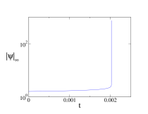
(A) $d=1,\sigma=6$, $\psi_{0}=1.6e^{-x^{2}}$

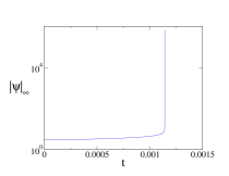
(B) $d=2,\sigma=3$, $\psi_{0}=3e^{-r^{2}}$

Figure 1: Maximal amplitude of singular solutions of the supercritical BNLS.

The radially-symmetric BNLS (7) was solved in the supercritical cases:

1. $d=1,\sigma=6$ with the initial condition $\psi_{0}(x)=1.6e^{-x^{2}}$.

2. $d=2,\sigma=3$ with the initial condition $\psi_{0}(r)=3e^{-r^{2}}$.

In both cases, the solutions blowup at a finite time, see Figure 1.

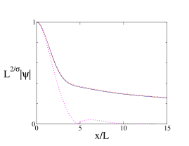
(A) $d=1,\sigma=6$

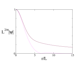
(B) $d=2,\sigma=3$

Figure 2: The solutions of Figure 1, rescaled according to (29), at the focusing levels $1/L=10^{4}$ (blue solid line) and $1/L=10^{8}$ (black dashed line). The red dash-dotted line is the rescaled solution ${S_{\text{\tiny B}}}$ of (28). The magenta dotted line is the rescaled ground-state $R$.

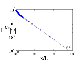
(A) $d=1,\sigma=6$

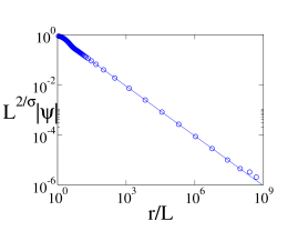
(B) $d=2,\sigma=3$

Figure 3: The solutions of Figure 1, rescaled according to (29), at the focusing level $1/L=10^{8}$ (circles). Solid lines are the fitted curves $y=0.63\cdot(x/L)^{-0.33}$ (left) and $y=0.85\cdot(r/L)^{-0.66}$ (right).

To check whether the solutions collapse with the self-similar profile (28), the solution was rescaled according to

$$\psi_{\text{rescaled}}(t,\rho)=L^{2/\sigma}(t)\psi(t,r=\rho\cdot L),\qquad L(t)={\left\|{\psi}\right\|}_{\infty}^{-2/\sigma}.$$ (29)

Comparing this rescaling with (28b) shows that it implies that $|{S_{\text{\tiny B}}}(0)|={\left\|{{S_{\text{\tiny B}}}}\right\|}_{\infty}=1$. This requirement can always be satisfied with a proper choice of $\nu$, see (15). Figure 2A shows the rescaled solutions at the focusing levels $L=10^{-4}$ and $L=10^{-8}$, and the rescaled solution ${S_{\text{\tiny B}}}(\rho)$ of (28). The three curves are indistinguishable, showing that the solution is self-similar with the ${S_{\text{\tiny B}}}$ profile, and not with the ${R_{\text{\tiny B}}}$ profile. As additional evidence, Figure 3 shows that as $\rho\to\infty$, the self-similar profile of $\psi$ decays as $\rho^{-2/\sigma}$, which is in agreement with the decay rate of ${S_{\text{\tiny B}}}_{,1}(\rho)$.

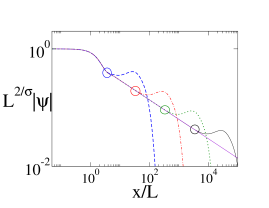
(A) $d=1,\sigma=6$

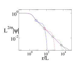
(B) $d=2,\sigma=3$

Figure 4: Convergence to a self-similar profile. The solutions of Figure 1, rescaled according to (29), as a function of $\log(r/L)$, at the focusing levels $L=10^{-1}$ (dashed blue line), $L=10^{-2}$ (dash-doted red line), $L=10^{-3}$ (dotted green line), $L=10^{-4}$ (solid black line) and $L=10^{-8}$ (solid magenta line). The circles mark the approximate position where each curve bifurcates from the limiting profile, see also Table 1.

$1/L$	$10$	$100$	$1000$	$10000$	$r_{c}$
$x/L~{}(d=1)$	$3.6$	$36$	$360$	$3600$	$0.36$
$r/L~{}(d=2)$	$6$	$60$	$600$	$6000$	$0.6$

Table 1: Position of circles in Figure 3.

We next verify that the solution converges to the asymptotic profile for $r\in[0,r_{c}]$, i.e., for $\rho\in[0,r_{c}/L(t)]$. To do this, we plot in Figure 4 the rescaled solution at focusing levels of $1/L=10,100,1000,10000$, as a function of $\log(r/L)$. The curves are indistinguishable at $r/L=\mathcal{O}(1)$, but bifurcate at increasing values of $r/L$. These “bifurcations positions” are marked by circles in Figure 4, and their $r/L$ values are listed in Table 1. The “bifurcation positions” are linear in $1/L$, indicating that the region where $\psi\sim\psi_{S_{\text{\tiny B}}}$ is indeed $\rho\in[0,r_{c}/L(t)]$, which corresponds to $r\in[0,r_{c}]$.

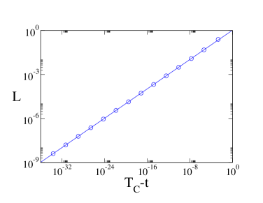
(A) $d=1,\sigma=6$

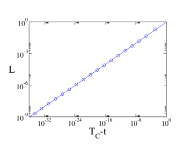
(B) $d=2,\sigma=3$

Figure 5: $L(t)$ as a function of $\left.({T_{\rm c}}-t)\right.$, on a logarithmic scale, for the solutions of Figure 1 (circles). Solid lines are the fitted curves $\left.L=1.048\cdot({T_{\rm c}}-t)^{0.2502}\right.$ (A) and $\left.L=0.931\cdot({T_{\rm c}}-t)^{0.2504}\right.$ (B).

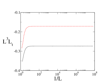
(A)

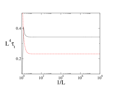
(B)

Figure 6: A: $L^{3}L_{t}$ as a function of $1/L$, for the solution of Figure 1A (black solid line) and of Figure 1B (red dashed line). B: Same as (A) for $L^{4}\tau_{t}$, where $\tau=\arg\psi(t,r=0)$.

In order to compute the blowup rate $p$, we performed a least-squares fit of $\log(L)$ with $\log(T_{c}-t)$, see Figure 5. The resulting values are $p\approx 0.2502$ in the $d=1,\sigma=6$ case, and $p\approx 0.2504$ in the $d=2,\sigma=3$ case. Next, we provide two indications that the blowup rate is exactly $1/4$, i.e., that

$$L(t)\sim\kappa\sqrt[4]{{T_{\rm c}}-t},\qquad\kappa>0.$$

1. If the blowup rate is exactly a quartic root, then $L^{3}L_{t}\to-\frac{\kappa^{4}}{4}<0.$ Indeed, Figure 6A shows that in the case $d=1$, $\sigma=6$, $L^{3}L_{t}\to-0.289$, implying that

   $$\kappa^{\rm admis.}(d=1,\sigma=6)\approx\sqrt[4]{4\cdot 0.289}\approx 1.037\,.$$ (30a)

   In the case $$d=2 \sigma=3 L^{3}L_{t}\to-0.171$$, , , implying that

   $$\kappa^{\rm admis.}(d=2,\sigma=3)\approx\sqrt[4]{4\cdot 0.171}\approx 0.909\,.$$ (30b)

   Since $L^{3}L_{t}$ converges to a finite, negative constant, this shows that the blowup rate is exactly $1/4$.

2. According to Lemma 10, if $\lim_{t\to T_{c}}L^{3}L_{t}<0$, the self-similar profile ${S_{\text{\tiny B}}}(\rho)$ does not satisfy the standing-wave equation (26), but rather is a solution to the problem (28c), as is clearly demonstrated in Figure 2.

We recall that calculation of the profile ${S_{\text{\tiny B}}}$ requires knowing the numerical values for $\nu$ and $\kappa$, see Appendix A. The value of $\kappa$ was obtained previously from the limit $\lim_{t\to T_{c}}(-4L^{3}L_{t})^{1/4}$. We approximate the value of the coefficient $\nu$ from

$$\nu_{\text{numeric}}=\lim_{t\to{T_{\rm c}}}L^{4}(t)\frac{d\tau}{dt},\qquad\tau=\arg\psi(t,r=0).$$ (31)

Indeed, Figure 6B shows that in both cases $L^{4}(t)\frac{d\tau}{dt}$ quickly converge to

$$\nu_{\text{numeric}}(d=1,\sigma=6)=0.36187,\qquad\nu_{\text{numeric}}(d=2,\sigma=3)=0.22826.$$ (32)

As a further verification, using the above values for $\nu$, we seek a value of $\kappa$ such that the solution of (28c) will satisfy $|{S_{\text{\tiny B}}}(0)|=1$, and obtain

$$\kappa(d=1,\sigma=6,\nu=0.36187)=1.007,\quad\kappa(d=2,\sigma=3,\nu=0.22826)=0.894.$$

These values are within 1%–3% from the values of $1.037$ and $0.909$ we obtained directly from the BNLS simulations, see (30).

Finally, we verified that the value of $\kappa$ in the blowup rate (28d) is universal. We solve the BNLS in the case $d=1,\sigma=6$ with the initial condition $\psi_{0}(x)=2e^{-x^{4}}$. In this case, the calculated value of $\kappa(d=1,\sigma=6)$ is $\kappa=\displaystyle\lim_{t\to{T_{\rm c}}}\sqrt[4]{-4L_{t}L^{3}}\approx 1.037$, which is equal, to first $3$ significant digits, to the previously obtained value, see (30a), for the initial condition $\psi_{0}(x)=1.6e^{-x^{2}}$. Similarly, in the case $d=2,\sigma=3$, we solve the equation with the initial condition $\psi_{0}(x)=3e^{-x^{4}}$. The calculated value of $\kappa(d=2,\sigma=3)$ is $\kappa=\displaystyle\lim_{t\to{T_{\rm c}}}\sqrt[4]{-4L_{t}L^{3}}\approx 0.913$, which is equal, to first $2$ significant digits, to the previously obtained value, see (30b), for the initial condition $\psi_{0}(x)=3e^{-x^{2}}$.

Acknowledgments

We thank Nir Gavish for useful discussions, and Elad Mandelbaum for preliminary numerical calculations. This research was partially supported by grant #123/2008 from the Israel Science Foundation (ISF).

Appendix A Numerical calculation of the ${S_{\text{\tiny B}}}$ profile

In order to solve equation (28c), we first define its linear part, which is the fourth-order linear differential operator $$L\left[S\right]$$

$$L\left[S(\rho)\right] = -\nu S(\rho)+i\frac{\kappa^{4}}{4}\left(\frac{2}{\sigma}S+\rho S^{\prime}\right)-\Delta_{\rho}^{2}S,$$ (33a)

under the BCs, see equation (24),

$$\begin{gathered}S^{\prime}(0)=S^{\prime\prime\prime}(0)=S(\infty)=0,\qquad\lim_{\rho\to\infty}\rho^{\gamma}\left(\rho S^{\prime}+\left(\frac{2}{\sigma}+i\frac{4\nu}{\kappa^{4}}\right)S\right)=0\\ \gamma_{0}<\gamma<\gamma_{1},\qquad\gamma_{0}=\frac{2}{3}\left(d-2-\frac{2}{\sigma}\right),\quad\gamma_{1}=4+\frac{2}{\sigma}.\end{gathered}$$ (33b)

The nonlinear ODE (28c) is therefore rewritten as

$$L\left[S(\rho)\right]+\left|S\right|^{2\sigma}S=0.$$ (34)

For given numerical values of $\nu$ and $\kappa$, we wish to calculate the ground state of the nonlinear boundary-value problem (34). In order to do so, we modify the SLSR method for the calculation of the ground-state of the NLS [Pet76, PS01, AM05] and BNLS [BFM10b] as follows. We consider the fixed-point iterative scheme

$$S^{\left(k+1\right)}\left(\rho\right)=-L^{-1}\left[\left|S^{\left(k\right)}\right|^{2\sigma}S^{\left(k\right)}\right],\qquad k=0,1,\dots$$ (35)

for the solution of (34). In the standard application of the SLSR method, $L$ is a differential operator of constant coefficients, and its inversion is easily performed using the Fourier transform. In our case, $L$ is a variable-coefficient operator, and the Fourier Transform cannot be used. Therefore, we discretize the operator $L$ using finite differences, see Appendix  A.1, and invert it using the LU decomposition.

We observe numerically that generically, the iterations (35) converge to zero for a small initial guess and diverge to infinity for a large initial guess. To avoid this divergence, we rescale the approximate solutions at each iteration, so that they satisfy the integral relation:

$$\int|S|^{2}\rho^{d-1}d\rho=\langle S,S\rangle=-\text{Re}\langle S,L^{-1}|S|^{2\sigma}S\rangle,$$

which follows from multiplication of (35) by $S$. Here, $<\cdot>$ denotes the standard inner product $\langle f,g\rangle=\int f^{*}g\rho^{d-1}d\rho$. Following a similar argumentation as in [BFM10b], we obtain that the iterations are

$$S^{(k+1)}=-\left(\frac{-\langle S^{(k)},S^{(k)}\rangle}{\text{Re}\left\langle S^{(k)},L^{-1}|S^{(k)}|^{2\sigma}S^{(k)}\right\rangle}\right)^{1+\frac{1}{2\sigma}}L^{-1}\left[|S^{(k)}|^{2\sigma}S^{(k)}\right].$$ (36)

In our simulation, this method converged for every value of $\nu$ and $\kappa$ that we tried. The numerical values of $\nu$ was obtained from the on-axis phase of the BNLS simulation solutions, as explained in Section 3.2. In order to obtain a prediction of $\kappa$, we recall that the specific choice (29) of the blowup rate $L(t)$ implies that $|{S_{\text{\tiny B}}}(0)|=1$. We therefore use the SLSR solver to search for the value of $\kappa$ for which $|{S_{\text{\tiny B}}}(0)=1|$.

A.1 Discretization of $L$

Using half-integer grid

$$\rho_{n}=\left(n+\frac{1}{2}\right)h,\qquad n=0,\dots N-1,\qquad h=\frac{R_{\max}}{N},$$

the ${\cal O}\left(h^{2}\right)$ centered-difference discretizations of the radial biharmonic operator $D_{\rho}^{2}$ and of the first-derivative, the approximation at the interior nodes is

$$\left(-\nu+\frac{i\kappa^{4}}{2\sigma}\right)S_{n}+\frac{i\kappa^{4}}{4}\rho_{n}\frac{S_{n+1}-S_{n-1}}{2h}-D_{\rho}^{2}S_{n}+\left|S_{n}\right|^{2\sigma}S_{n} = {\cal O}\left(h^{2}\right).$$

The stencil is five-nodes wide, so two ghost-nodes are needed at each boundary. In order to enfold the ghost-nodes at $\rho=0$, we relate them to the interior nodes, using the symmetry of the solution $S(\rho)=S(-\rho)$, so that

$$\left[\begin{array}[]{c}S_{-2}\\ S_{-1}\end{array}\right]=\left[\begin{array}[]{cc}0&1\\ 1&0\end{array}\right]\left[\begin{array}[]{c}S_{0}\\ S_{1}\end{array}\right].$$

This relation is substituted in the discretization of the equation at $\rho_{0}$ and $\rho_{1}$.

At the other boundary $\rho=R_{\max}$ we use the approximate form of the solution obtained from the WKB approximation, i.e., we require

$$S_{n}=c_{1}{S_{\text{\tiny B}}}_{,1}(\rho_{n})+c_{4}{S_{\text{\tiny B}}}_{,4}(\rho_{n}),\qquad n=N-2,N-1,N,N+1,\dots.$$

In matrix form, this becomes

$$\left[\begin{array}[]{cc}{S_{\text{\tiny B}}}_{,1}(\rho_{N-1})&{S_{\text{\tiny B}}}_{,4}(\rho_{N-1})\\ {S_{\text{\tiny B}}}_{,1}(\rho_{N})&{S_{\text{\tiny B}}}_{,4}(\rho_{N})\\ {S_{\text{\tiny B}}}_{,1}(\rho_{N+1})&{S_{\text{\tiny B}}}_{,4}(\rho_{N+1})\\ {S_{\text{\tiny B}}}_{,1}(\rho_{N+2})&{S_{\text{\tiny B}}}_{,4}(\rho_{N+2})\end{array}\right]\left[\begin{array}[]{c}c_{1}\\ c_{4}\end{array}\right]=\left[\begin{array}[]{c}S_{N-1}\\ S_{N}\\ S_{N+1}\\ S_{N+2}\end{array}\right]$$

which is then solved to obtain

$$\left[\begin{array}[]{c}S_{N+1}\\ S_{N+2}\end{array}\right]=\left[\begin{array}[]{cc}{S_{\text{\tiny B}}}_{,1}(\rho_{N+1})&{S_{\text{\tiny B}}}_{,4}(\rho_{N+1})\\ {S_{\text{\tiny B}}}_{,1}(\rho_{N+2})&{S_{\text{\tiny B}}}_{,4}(\rho_{N+2})\end{array}\right]\left[\begin{array}[]{cc}{S_{\text{\tiny B}}}_{,1}(\rho_{N-1})&{S_{\text{\tiny B}}}_{,4}(\rho_{N-1})\\ {S_{\text{\tiny B}}}_{,1}(\rho_{N})&{S_{\text{\tiny B}}}_{,4}(\rho_{N})\end{array}\right]^{-1}\left[\begin{array}[]{c}S_{N-1}\\ S_{N}\end{array}\right].$$

Some care should be taken when choosing the parameters $R_{\max}$ and $N$. On the one hand, we use the closed-form approximations for ${S_{\text{\tiny B}}}_{,1}$ and ${S_{\text{\tiny B}}}_{,4}$ that become more accurate for $R_{\max}\gg 1$. On the other hand, since ${S_{\text{\tiny B}}}_{,4}$ has a super-exponentially decreasing term $e^{-\rho^{4/3}}$, choosing too-large a value of $R_{\max}$ leads to numerical instabilities. Finally, in order to resolve the rapid-oscillations $e^{i\rho^{4/3}}$ of ${S_{\text{\tiny B}}}_{,4}$, the grid-size $N$ must be chosen such that $\rho^{1/3}h_{\rho}=\mathcal{O}\left(R_{\max}^{4/3}/N\right)\ll 1$, hence that $\left.N\geq\mathcal{O}\left(R_{\max}^{4/3}\right)\right.$. The grid-size $N$, however, cannot be arbitrarily large, since the condition number of $L$ is $\mathcal{O}\left(N^{4}\right)$.

In the simulations presented in this study, we used an extension of above approach to a fourth-order approximation, and set $R_{\max}=160$ and $N=32000$.

References

- [AM05] MJ Ablowitz and ZH Musslimani. Spectral renormalization method for computing self-localized solutions to nonlinear systems. Opt. Lett., 30(16):2140–2142, 2005.
- [BAKS00] M. Ben-Artzi, H. Koch, and J.-C. Saut. Dispersion estimates for fourth order Schrödinger equations. C. R. Acad. Sci. Paris Sér. I Math., 330:87–92, 2000.
- [BFG10] G. Baruch, G. Fibich, and N. Gavish. Singular standing ring solutions of nonlinear partial differential equations. Physica D, 239(20):1968–1983, 2010.
- [BFM10a] G. Baruch, G. Fibich, and E. Mandelbaum. Ring-type singular solutions of the biharmonic nonlinear Schrödinger equation. Nonlinearity, 23(11):2867, 2010.
- [BFM10b] G. Baruch, G. Fibich, and E. Mandelbaum. Singular solutions of the -critical biharmonic nonlinear Schrödinger equation. SIAM J. of App. Math., to appear, 2010.
- [BP92] L. Bergé and D. Pesme. Time dependent solutions of wave collapse. Phys. Lett. A, 166:116–122, 1992.
- [Bud01] C. J. Budd. Asymptotics of multibump blow-up self-similar solutions of the nonlinear Schrödinger equation. SIAM J. Appl. Math., 62:801–830 (electronic), 2001.
- [CHL11] M. Chae, S. Hong, and S. Lee. Mass concentration for the -critical Nonlinear Schrodinger equations of higher orders. Discrete and Continuous Dynamical Systems (DCDS-A), 29(3):909 – 928, 2011.
- [DG09] A. Ditkowsky and N. Gavish. A grid redistribution method for singular problems. J. Comp. Phys., 228:2354–2365, 2009.
- [FIP02] Gadi Fibich, Boaz Ilan, and George Papanicolaou. Self-focusing with fourth-order dispersion. SIAM J. Applied Math., 62(4):1437–1462, 2002.
- [KL95] N. Koppel and M. Landman. Spatial structure of the focusing singularity of the nonlinear Schrödinger equation: a geometrical analysis. SIAM J. Appl. Math., 55:1297–1323, 1995.
- [LPSS88] B.J. LeMesurier, G. Papanicolaou, C. Sulem, and P.L. Sulem. Focusing and multi-focusing solutions of the nonlinear Schrödinger equation. Physica D, 31:78–102, 1988.
- [MRS09] F. Merle, P. Raphael, and J. Szeftel. Stable self similar blow up dynamics for slightly supercritical NLS equations. preprint http://arXiv.org/abs/0907.4098, 2009.
- [MXZ08] Changxing Miao, Guixiang Xu, and Lifeng Zhao. Global wellposedness and scattering for the defocusing energy-critical nonlinear Schrodinger equations of fourth order in dimensions . arXiv preprint, 2008.
- [MXZ09] Changxing Miao, Guixiang Xu, and Lifeng Zhao. Global well-posedness and scattering for the focusing energy-critical nonlinear Schrödinger equations of fourth order in the radial case. J. of Differ. Equations, 246(9):3715 – 3749, 2009.
- [Pau07] B. Pausader. Global well-posedness for energy critical fourth-order Schrodinger equations in the radial case. Dynamics of PDE, 4(3):197–225, 2007.
- [Pau09a] Benoit Pausader. The cubic fourth-order Schrödinger equation. Journal of Functional Analysis, 256(8):2473 – 2517, 2009.
- [Pau09b] Benoit Pausader. The focusing energy-critical fourth-order Schrödinger equation with radial data. Discrete and continuous dynamical systems, 24(4):1275–1292, August 2009.
- [Pet76] V. I. Petviashvili. Equation of an extraordinary soliton. Sov. J. Plasma Phys., 2:469–472, June 1976.
- [PS01] Dmitry B. Pelinovsky and Yury A. Stepanyants. convergence of petviashvili’s iteration method for numerical approximation of stationary solutions of nonlinear wave equations. SIAM Journal on Numerical Analysis, 42(3):1110 – 1127, 20040601.
- [RW00] W. Ren and X.P. Wang. An iterative grid redistribution method for singular problems in multiple dimensions. J. Comput. Phys., 159:246–273, 2000.
- [SKL93] V.F. Shvets, N.E. Kosmatov, and B.J. LeMesurier. On collapsing solutions of the nonlinear Schrödinger equation in supercritical case. In R.E. Caflisch and G.C. Papanicolaou, editors, Singularities in Fluids, Plasmas and Optics, pages 317–321. Kluwer, 1993.
- [SS99] C. Sulem and P.L. Sulem. The Nonlinear Schrödinger Equation. Springer, New-York, 1999.
- [ZZY10] S. Zhu, J. Zhang, and H. Yang. Limiting profile of the blow-up solutions of the fourth-order Nonlinear Schrodinger equation. Dynamics of PDE, 7(2):187 – 205, 2010.