Dynamic Growth Estimates of Maximum Vorticity for 3D Incompressible Euler Equations and the SQG Model

Abstract

By performing estimates on the integral of the absolute value of vorticity along a local vortex line segment, we establish a relatively sharp dynamic growth estimate of maximum vorticity under some assumptions on the local geometric regularity of the vorticity vector. Our analysis applies to both the 3D incompressible Euler equations and the surface quasi-geostrophic model (SQG). As an application of our vorticity growth estimate, we apply our result to the 3D Euler equation with the two anti-parallel vortex tubes initial data considered by Hou-Li [12]. Under some additional assumption on the vorticity field, which seems to be consistent with the computational results of [12], we show that the maximum vorticity can not grow faster than double exponential in time. Our analysis extends the earlier results by Cordoba-Fefferman [6, 7] and Deng-Hou-Yu [8, 9].

Keywords 3D Euler equations; SQG equation; Finite time blow-up; Growth rate of maximum vorticity; Geometric properties.

Mathematics Subject Classification Primary 76B03; Secondary 35L60, 35M10

1 Introduction

One of the most challenging problems in mathematical fluid dynamics is to understand whether a solution of the 3D incompressible Euler equations can develop a finite time singularity from smooth initial data with finite energy. A main difficulty is due to the presence of the vortex stretching term, which has a formal quadratic nonlinearity in vorticity. This problem has attracted a lot of attention in the mathematics community and many people have contributed to its understanding, see the recent book by Majda and Bertozzi [15] for a review of this subject.

An important development in recent years is the work by Constantin, Fefferman, and Majda who showed that the local geometric regularity of vortex lines can lead to depletion of nonlinear vortex stretching [2]. Inspired by the work of [2], Deng, Hou, and Yu [8, 9] obtained more localized non-blowup criteria by exploiting the geometric regularity of a vortex line segment whose arclength may shrink to zero at the potential singularity time. To obtain these results, Deng-Hou-Yu [8, 9] used a Lagrangian approach and explored the connection between the local geometric regularity of vortex lines and the growth of vorticity. Guided by this local geometric non-blowup analysis, Hou and Li [12, 13] performed large scale computations with resolution up to $1536\times 1024\times 3072$ to re-examine some of the most well-known blow-up scenarios, including the two slightly perturbed anti-parallel vortex tubes that was originally investigated by Kerr [14]. The computations of Hou and Li [12] provide strong numerical evidence that the geometric regularity of vortex lines, even in an extremely localized region near the support of maximum vorticity, can lead to depletion of vortex stretching. We refer to a recent survey paper [11] for more discussions on this topic.

In this paper, we derive new growth rate estimates of maximum vorticity for the 3D incompressible Euler equations. We use a framework similar to that adopted by Deng-Hou-Yu [8]. The main innovation of this work is to introduce a method of analysis to study the dynamic evolution of the integral of the absolute value of vorticity along a local vortex line segment. Specifically, we derive a dynamic estimate for the quantity:

$$Q(t)=\frac{1}{L(t)}\int_{0}^{L(t)}|\omega(\mathbf{x}(s,t),t)|ds,$$ (1)

where $\mathbf{x}(s,t)$ is a parameterization of a vortex line segment, $L^{t}$, and $L(t)$ is the arclength of $L^{t}$. The assumption on $\mathbf{x}(s,t)$ is less restrictive than that in [8]. As in [8], we assume that the vorticity along $L^{t}$ is comparable to the maximum vorticity, i.e. $\max_{L^{t}}|\omega|\geq c_{0}\|\omega\|_{L^{\infty}}$. Let $V(t)=\max_{\mathbf{x}\in L^{t}}|(\mathbf{u}\cdot\mbox{\boldmath$\xi$})(\mathbf{x},t)|$, and $U(t)=\max_{\mathbf{x}\in L^{t}}|(\mathbf{u}\cdot\mbox{\boldmath$\xi$}^{\bot})(\mathbf{x},t)|$. Here $\xi$ be the unit vorticity vector of $L^{t}$, and $\mbox{\boldmath$\xi$}^{\bot}$ the unit normal vector. Under the assumption that $\int_{L^{t}}|\mbox{\boldmath$\xi$}\cdot\nabla\mbox{\boldmath$\xi$}|ds\leq C_{0}$ and $\int_{L^{t}}|\nabla\cdot\mbox{\boldmath$\xi$}|ds\leq C_{0}$, we derive a relatively sharp growth estimate for $Q(t)$, which can be used to obtain an upper bound on the growth rate of the maximum vorticity:

$$\|\omega(t)\|_{L^{\infty}}\leq\frac{Q(T_{0})}{c_{0}}\exp\left(C_{0}+\int_{T_{0}}^{t}\frac{C_{V}V(t^{\prime})+C_{U}U(t^{\prime})}{L(t^{\prime})}dt^{\prime}\right),$$ (2)

where $C_{U}$ and $C_{V}$ depend on $C_{0}$. If we further assume that $L(t)$ has a positive lower bound, the above estimate implies no blow-up up to $t=T$, if $\int_{0}^{T}\|\mathbf{u}\|_{\infty}dt<\infty$. This generalizes the result of Cordoba and Fefferman [6].

The above estimate extends the result of Deng-Hou-Yu in [8]. In fact, it is easy to check that under the assumption that $U(t)+V(t)\leq C_{u}(T-t)^{-A}$ and $L(t)\geq C_{L}(T-t)^{B}$ with $A+B<1$, the right hand side of (2) remains bounded up to the time $t=T$, implying no blow-up up to $t=T$. Our result can be also applied to the critical case when $A+B=1$, which was considered in [9]. In this case, we have

$$\displaystyle\frac{C_{V}V(t)+C_{U}U(t)}{L(t)}\sim\frac{1}{T-t}.$$ (3)

If we further assume that there exists $C_{w}<1$ such that

$$\displaystyle\frac{C_{V}V(t)+C_{U}U(t)}{L(t)}\leq\frac{C_{w}}{T-t},$$ (4)

where $C_{w}$ depends on $C_{0}$, and the scaling constants in $U(t)$, $V(t)$ and $L(t)$, then our growth estimate implies that

$$\|\omega(t)\|_{L^{\infty}}\leq\frac{C}{(T-t)^{C_{w}}}.$$ (5)

Application of the Beale-Kato-Majda non-blow-up criterion [1] would exclude blow-up at $t=T$ since $C_{w}<1$ implies $\int_{0}^{T}\|\omega(t)\|_{L^{\infty}}dt<\infty$.

Of particular interest is the case when the vorticity has a local Clebsch representation. In this case, the vorticity can be represented by the two Clebsch variables $\phi$ and $\psi$ near the support of maximum vorticity as follows:

$$\omega=\nabla\phi\times\nabla\psi,$$ (6)

where $\phi$ and $\psi$ are carried by the flow, that is

$$\phi_{t}+{\bf u}\cdot\nabla\phi=0,$$ (7)

$$\psi_{t}+{\bf u}\cdot\nabla\psi=0,$$ (8)

where ${\bf u}$ is the velocity field. In addition to the geometric regularity assumption on $L^{t}$, if we further assume that one of the Clebsch variables has a bounded gradient and $L(t)\geq L_{0}>0$, then we prove that the maximum vorticity can not grow faster than double exponential in time, i.e. $\|\omega(t)\|_{L^{\infty}}\leq C\exp(\exp(c_{0}t))$.

As an application of this result, we re-examine the computations of the 3D incompressible Euler equations with the two slightly perturbed anti-parallel vortex tubes initial data by Hou and Li [12]. By examining the vorticity field carefully near the support of maximum vorticity (see Fig. 1), the vorticity field seems to have a local Clebsch representation. One of the Clebsch variables may be chosen along the vortex tube direction, which appears to be regular. Moreover, the vortex lines within the support of maximum vorticity seem to be quite smooth and has length of order one, implying that $L(t)$ has a positive lower bound. Thus the result that we described above may apply. One of the important findings of the Hou-Li computations is that the maximum vorticity does not grow faster than double exponential in time. Our new estimate on the vorticity growth may offer a theoretical explanation to the mechanism that leads to this dynamic depletion of vortex stretching.

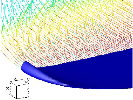
Figure 1: The local 3D vortex structures and vortex lines around the maximum vorticity at $t=17$. Computation from Hou and Li [12] for the 3D incompressible Euler equations with two slightly perturbed anti-parallel vortex tubes initial data.

We also apply our method of analysis to the surface quasi-geostrophic model (SQG) [3]. As pointed out in [3], a formal analogy between the SQG model and the 3D Euler equations can be established by considering $\nabla^{\bot}\theta$ as the corresponding vorticity in the 3D Euler equations. Here $\theta$ is a scalar quantity that is transported by the flow:

$$\theta_{t}+{\bf u}\cdot\nabla\theta=0,\quad{\bf u}=\nabla^{\bot}(-\Delta)^{-1/2}\theta.$$ (9)

Let $L^{t}$ be a level set segment of $\theta$ along which $|\nabla^{\bot}\theta|$ is comparable to $\|\nabla^{\bot}\theta\|_{L^{\infty}}$ and denote by $\xi$ the unit tangent vector of $L^{t}$. Under the assumption that $\int_{L^{t}}|\mbox{\boldmath$\xi$}\cdot\nabla\mbox{\boldmath$\xi$}|ds\leq C_{0}$ and $\int_{L^{t}}|\nabla\cdot\mbox{\boldmath$\xi$}|ds\leq C_{0}$, we obtain a much better growth estimate for $\|\nabla^{\bot}\theta\|_{L^{\infty}}$:

$$\|\nabla^{\bot}\theta(t)\|_{L^{\infty}}\leq C\exp\left(c_{1}\exp\left(\int_{T_{0}}^{t}\frac{c_{2}}{L(t^{\prime})}dt^{\prime}\right)\right).$$ (10)

In particular, if $L(t)\geq L_{0}>0$, the above estimate implies that $\|\nabla^{\bot}\theta\|_{L^{\infty}}\leq C\exp(\exp(c_{0}t))$. This seems to be consistent with the numerical results obtained in [16, 4], see also [7, 10].

The rest of the paper is organized as follows. In Section 2, we derive our estimate on the integral of vorticity over a vortex line segment for the 3D Euler equations, and apply this estimate to obtain an upper bound for the dynamic growth rate of maximum vorticity. In Section 3, we generalize our analysis to the SQG model. In the Appendix, we prove a technical result for the 3D Euler equations which states that the maximum velocity is bounded by $C\log(\|\omega(t)\|_{L^{\infty}})$ when the vorticity field has a local Clebsch representation and one of the Clebsch variables has a bounded gradient.

2 Vorticity growth estimate for the 3D Euler equations

In this section, we derive a new dynamic growth estimate of the maximum vorticity for the 3D incompressible Euler equations. We adopt a framework similar to that used in [8]. Let $\Omega(t)=\|\omega(t)\|_{L^{\infty}}$. We consider, at time $t$, a vortex line segmant $L^{t}$ along which the maximum of $|\omega|$ (denoted by $\Omega_{L}(t)$ in the following) is comparable to $\Omega(t)$. We use $\mathbf{x}(s,t),\;0\leq s\leq L(t)$ to parameterize $L^{t}$ with $s$ being the arclength variable. In our paper, we do not assume that $L^{t}$ is a subset of $\mathbf{X}(L^{t^{\prime}},t^{\prime},t)$, the flow image of $L^{t^{\prime}}$ at time $t$, for $t^{\prime}<t$. This assumption was required in the analysis of [8]. Further, we denote by $L(t)$ the arclength of $L^{t}$. The unit tangential and normal vectors are defined as follows:$\mbox{\boldmath$\xi$}=\frac{\nabla^{\bot}\theta}{|\nabla^{\bot}\theta|},\;\mbox{\boldmath$\xi$}^{\bot}=\frac{\mbox{\boldmath$\xi$}\cdot\nabla\mbox{\boldmath$\xi$}}{|\mbox{\boldmath$\xi$}\cdot\nabla\mbox{\boldmath$\xi$}|}$, the unsigned curvature is defined as $\kappa=|\mbox{\boldmath$\xi$}\cdot\nabla\mbox{\boldmath$\xi$}|$, and $\tau=\nabla\cdot\mbox{\boldmath$\xi$}$. Finally, we denote $V(t)=\max_{\mathbf{x}\in L^{t}}|(\mathbf{u}\cdot\mbox{\boldmath$\xi$})(\mathbf{x},t)|$, and $U(t)=\max_{\mathbf{x}\in L^{t}}|(\mathbf{u}\cdot\mbox{\boldmath$\xi$}^{\bot})(\mathbf{x},t)|$.

Lemma 2.1

Let $L^{t}=\left\{\mathbf{x}(s,t),0\leq s\leq L(t)\right\}$ be a family of vortex line segments which come from the same vortex line. Define $Q(t)$ as the mean of $|\omega(\mathbf{x},t)|$ over $L^{t}$,

$$Q(t)=\frac{1}{L(t)}\int_{0}^{L(t)}|\omega(\mathbf{x}(s,t),t)|ds.$$ (11)

Then, we have

$$\frac{dQ(t)}{dt} = \frac{1}{L}\left(\int_{0}^{L(t)}2\tau|\omega|(\mathbf{u}\cdot\mbox{\boldmath$\xi$})ds-\int_{0}^{L(t)}\kappa|\omega|(\mathbf{u}\cdot\mbox{\boldmath$\xi$}^{\bot})ds\right.$$ (12)

$$\left.-\int_{0}^{L(t)}\kappa\left(|\omega|(\mathbf{x}(s,t),t)-|\omega|(\mathbf{x}(L(t),t),t)\right)(\mathbf{u}\cdot\mbox{\boldmath$\xi$}^{\bot})ds\right)$$

$$+\frac{1}{L}\left[\left(\mathbf{u}\cdot\mbox{\boldmath$\xi$}\right)(\mathbf{x}(L,t),t)-\left(\mathbf{u}\cdot\mbox{\boldmath$\xi$}\right)(\mathbf{x}(0,t),t)\right]|\omega|(\mathbf{x}(L,t),t)$$

$$+\frac{1}{L}\left[|\omega(\mathbf{x}(L,t),t)|-|\omega(\mathbf{x}(0,t),t)|\right]\left(\frac{d\mathbf{x}}{dt}\cdot\mbox{\boldmath$\xi$}+\mathbf{u}\cdot\mbox{\boldmath$\xi$}\right)(\mathbf{x}(0,t),t)$$

$$+\frac{L_{t}}{L}\left(|\omega(\mathbf{x}(L,t),t)|-Q\right).\quad\quad$$

Proof  Differentiating $Q(t)$ with respect to $t$ yields

$$\frac{dQ(t)}{dt} = \frac{1}{L(t)}\frac{d}{dt}\left(\int_{0}^{L(t)}|\omega(\mathbf{x}(s,t),t)|ds\right)-\frac{QL_{t}}{L}.$$ (13)

Let $\beta$ be the arclength parameter of this vortex line at time $T_{0}$. Then we can write, for this specific vortex line, $s=s(\beta,t)$. Let $\beta_{1}(t),\beta_{2}(t)$ be the corresponding coordinates of the end points of $L^{t}$, i.e.

$$s(\beta_{1}(t),t)=0,\quad s(\beta_{2}(t),t)=L(t).$$

First, we can change the integral variable from $s$ to $\beta$ in (13),

$$\frac{d}{dt}\left(\int_{0}^{L(t)}|\omega(\mathbf{x}(s,t),t)|ds\right)=\frac{d}{dt}\left(\int_{\beta_{1}(t)}^{\beta_{2}(t)}|\omega(\mathbf{x}(s(\beta,t),t),t)|s_{\beta}d\beta\right).$$ (14)

In [8], Deng-Hou-Yu proved the following equality,

$$\frac{ds}{d\beta}(\mathbf{x}(\beta,t),t)=\frac{|\omega(\mathbf{x}(\beta,t),t)|}{|\omega(\mathbf{x}(\beta,T_{0}),T_{0})|}.$$ (15)

Substituting the above relation to (14) yields

$$\frac{d}{dt}\left(\int_{0}^{L(t)}|\omega(\mathbf{x}(s,t),t)|ds\right)$$ (16)

$$= \frac{d}{dt}\left(\int_{\beta_{1}(t)}^{\beta_{2}(t)}|\omega(\mathbf{x}(\beta,t),t)|^{2}/|\omega(\mathbf{x}(\beta,T_{0}),T_{0})|d\beta\right)$$

$$= \int_{\beta_{1}(t)}^{\beta_{2}(t)}\frac{2|\omega|}{|\omega(\mathbf{x}(\beta,T_{0}),T_{0})|}\frac{D}{Dt}|\omega|d\beta+\frac{|\omega(\mathbf{x}(\beta_{2},t),t)|^{2}}{|\omega(\mathbf{x}(\beta_{2},T_{0}),T_{0})|}\beta_{2t}-\frac{|\omega(\mathbf{x}(\beta_{1},t),t)|^{2}}{|\omega(\mathbf{x}(\beta_{1},T_{0}),T_{0})|}\beta_{1t}$$

$$= \int_{\beta_{1}(t)}^{\beta_{2}(t)}\frac{2|\omega|}{|\omega(\mathbf{x}(\beta,T_{0}),T_{0})|}\alpha|\omega|d\beta+\frac{|\omega(\mathbf{x}(\beta_{2},t),t)|^{2}}{|\omega(\mathbf{x}(\beta_{2},T_{0}),T_{0})|}\beta_{2t}-\frac{|\omega(\mathbf{x}(\beta_{1},t),t)|^{2}}{|\omega(\mathbf{x}(\beta_{1},T_{0}),T_{0})|}\beta_{1t}$$

$$= \int_{0}^{L(t)}2\alpha|\omega|ds+\frac{|\omega(\mathbf{x}(\beta_{2},t),t)|^{2}}{|\omega(\mathbf{x}(\beta_{2},T_{0}),T_{0})|}\beta_{2t}-\frac{|\omega(\mathbf{x}(\beta_{1},t),t)|^{2}}{|\omega(\mathbf{x}(\beta_{1},T_{0}),T_{0})|}\beta_{1t},$$

where we have used $\frac{D}{Dt}|\omega|=\alpha|\omega|$ with $\alpha=(\mbox{\boldmath$\xi$}\cdot\nabla)\mathbf{u}\cdot\mbox{\boldmath$\xi$}=(\mathbf{u}\cdot\mbox{\boldmath$\xi$})_{s}-\kappa\mathbf{u}\cdot\mbox{\boldmath$\xi$}^{\bot}$ [8].

Note that the arclength $L(t)$ can be expressed as follows:

$$L(t)=\int_{\beta_{1}(t)}^{\beta_{2}(t)}s_{\beta}d\beta=\int_{\beta_{1}(t)}^{\beta_{2}(t)}\frac{|\omega(\mathbf{x}(\beta,t),t)|}{|\omega(\mathbf{x}(\beta,T_{0}),T_{0})|}d\beta.$$ (17)

Differentiating the both sides with respect to $t$, we get

$$\frac{dL(t)}{dt} = \int_{\beta_{1}(t)}^{\beta_{2}(t)}\frac{D|\omega|/Dt}{|\omega(\mathbf{x}(\beta,T_{0}),T_{0})|}d\beta+\frac{|\omega(\mathbf{x}(\beta_{2},t),t)|\beta_{2t}}{|\omega(\mathbf{x}(\beta_{2},T_{0}),T_{0})|}-\frac{|\omega(\mathbf{x}(\beta_{1},t),t)|\beta_{1t}}{|\omega(\mathbf{x}(\beta_{1},T_{0}),T_{0})|}$$ (18)

$$= \int_{\beta_{1}(t)}^{\beta_{2}(t)}\frac{\alpha|\omega|}{|\omega(\mathbf{x}(\beta,T_{0}),T_{0})|}d\beta+\frac{|\omega(\mathbf{x}(\beta_{2},t),t)|\beta_{2t}}{|\omega(\mathbf{x}(\beta_{2},T_{0}),T_{0})|}-\frac{|\omega(\mathbf{x}(\beta_{1},t),t)|\beta_{1t}}{|\omega(\mathbf{x}(\beta_{1},T_{0}),T_{0})|}$$

$$= \int_{0}^{L(t)}\alpha ds+\frac{|\omega(\mathbf{x}(\beta_{2},t),t)|\beta_{2t}}{|\omega(\mathbf{x}(\beta_{2},T_{0}),T_{0})|}-\frac{|\omega(\mathbf{x}(\beta_{1},t),t)|\beta_{1t}}{|\omega(\mathbf{x}(\beta_{1},T_{0}),T_{0})|}.$$

Substituting the above relation to (14), we obtain

$$\frac{d}{dt}\left(\int_{0}^{L(t)}|\omega(\mathbf{x}(s,t),t)|ds\right)$$ (19)

$$= \int_{0}^{L(t)}2\alpha|\omega|ds+|\omega(\mathbf{x}(\beta_{2},t),t)|\left(L_{t}-\int_{0}^{L(t)}\alpha ds\right)$$

$$+\left(|\omega(\mathbf{x}(\beta_{2},t),t)|-|\omega(\mathbf{x}(\beta_{1},t),t)|\right)\frac{|\omega(\mathbf{x}(\beta_{1},t),t)|}{|\omega(\mathbf{x}(\beta_{1},T_{0}),T_{0})|}\beta_{1t}.$$

Observe that

$$\frac{d\mathbf{x}(0,t)}{dt}\cdot\mbox{\boldmath$\xi$}(\mathbf{x}(0,t),t) = \frac{d\mathbf{x}(\beta_{1}(t),t)}{dt}\cdot\mbox{\boldmath$\xi$}(\mathbf{x}(\beta_{1}(t),t),t)$$ (20)

$$= \left(\frac{\partial\mathbf{x}(\beta_{1},t)}{\partial t}+\frac{\partial\mathbf{x}(\beta_{1},t)}{\partial\beta_{1}}\frac{d\beta_{1}}{dt}\right)\cdot\mbox{\boldmath$\xi$}(\mathbf{x}(\beta_{1}(t),t),t)$$

$$= \left(\mathbf{u}(\beta_{1},t)+\frac{\omega(\mathbf{x}(\beta_{1},t),t)\beta_{1t}}{|\omega(\mathbf{x}(\beta_{1},T_{0}),T_{0})|}\right)\cdot\mbox{\boldmath$\xi$}(\mathbf{x}(\beta_{1}(t),t),t)$$

$$= \left(\mathbf{u}\cdot\mbox{\boldmath$\xi$}\right)(\mathbf{x}(0,t),t)+\frac{|\omega(\mathbf{x}(\beta_{1},t),t)|\beta_{1t}}{|\omega(\mathbf{x}(\beta_{1},T_{0}),T_{0})|}.$$

Substituting the above equality to (19), we get

$$\frac{d}{dt}\left(\int_{0}^{L(t)}|\omega(\mathbf{x}(s,t),t)|ds\right)$$ (21)

$$= \int_{0}^{L(t)}2\alpha|\omega|ds+|\omega(\mathbf{x}(L,t),t)|\left(L_{t}-\int_{0}^{L(t)}\alpha ds\right)$$

$$+\left(|\omega(\mathbf{x}(L,t),t)|-|\omega(\mathbf{x}(0,t),t)|\right)\left(\frac{d\mathbf{x}}{dt}\cdot\mbox{\boldmath$\xi$}-\mathbf{u}\cdot\mbox{\boldmath$\xi$}\right)(\mathbf{x}(0,t),t).$$

Now, we have

$$\frac{dQ(t)}{dt} = \frac{1}{L(t)}\frac{d}{dt}\left(\int_{0}^{L(t)}|\omega(\mathbf{x}(s,t),t)|ds\right)-\frac{QL_{t}}{L}$$ (22)

$$= \frac{1}{L(t)}\left(\int_{0}^{L(t)}2\alpha|\omega|ds-|\omega(\mathbf{x}(\beta_{2},t),t)|\int_{0}^{L(t)}\alpha ds\right)$$

$$+\frac{1}{L(t)}\left(|\omega(\mathbf{x}(\beta_{2},t),t)|-|\omega(\mathbf{x}(\beta_{1},t),t)|\right)\left(\frac{d\mathbf{x}}{dt}\cdot\mbox{\boldmath$\xi$}-\mathbf{u}\cdot\mbox{\boldmath$\xi$}\right)(\mathbf{x}(0,t),t)$$

$$+\frac{L_{t}}{L}\left(|\omega(\mathbf{x}(\beta_{2},t),t)|-Q\right).$$

Using $\alpha=(\mathbf{u}\cdot\mbox{\boldmath$\xi$})_{s}-\kappa\mathbf{u}\cdot\mbox{\boldmath$\xi$}^{\bot}$ and integrating by parts, we obtain

$$\int_{0}^{L(t)}2\alpha|\omega|ds-|\omega(\mathbf{x}(\beta_{2},t),t)|\int_{0}^{L(t)}\alpha ds$$ (23)

$$= \int_{0}^{L(t)}2|\omega|\left((\mathbf{u}\cdot\mbox{\boldmath$\xi$})_{s}-\kappa\mathbf{u}\cdot\mbox{\boldmath$\xi$}^{\bot}\right)ds-|\omega(\mathbf{x}(L,t),t)|\int_{0}^{L(t)}\left((\mathbf{u}\cdot\mbox{\boldmath$\xi$})_{s}-\kappa\mathbf{u}\cdot\mbox{\boldmath$\xi$}^{\bot}\right)ds$$

$$= 2\left(|\omega|\mathbf{u}\cdot\mbox{\boldmath$\xi$}\right)\left|{}_{0}^{L(t)}\right.+\int_{0}^{L(t)}2\tau|\omega|(\mathbf{u}\cdot\mbox{\boldmath$\xi$})ds-\int_{0}^{L(t)}2\kappa|\omega|\mathbf{u}\cdot\mbox{\boldmath$\xi$}^{\bot}ds$$

$$-|\omega|(\mathbf{x}(L,t),t)\left(\mathbf{u}\cdot\mbox{\boldmath$\xi$}\right)\left|{}_{0}^{L(t)}\right.+|\omega(\mathbf{x}(L,t),t)|\int_{0}^{L(t)}\kappa\mathbf{u}\cdot\mbox{\boldmath$\xi$}^{\bot}ds.$$

Substitute the above equality to (22) gives

$$\frac{dQ(t)}{dt} = \frac{1}{L}\left(\int_{0}^{L(t)}2\tau|\omega|(\mathbf{u}\cdot\mbox{\boldmath$\xi$})ds-\int_{0}^{L(t)}\kappa|\omega|(\mathbf{u}\cdot\mbox{\boldmath$\xi$}^{\bot})ds\right.$$ (24)

$$\left.-\int_{0}^{L(t)}\kappa\left(|\omega|(\mathbf{x}(s,t),t)-|\omega|(\mathbf{x}(L(t),t),t)\right)(\mathbf{u}\cdot\mbox{\boldmath$\xi$}^{\bot})ds\right)$$

$$+\frac{1}{L}\left[\left(\mathbf{u}\cdot\mbox{\boldmath$\xi$}\right)(\mathbf{x}(L,t),t)-\left(\mathbf{u}\cdot\mbox{\boldmath$\xi$}\right)(\mathbf{x}(0,t),t)\right]|\omega|(\mathbf{x}(L,t),t)$$

$$+\frac{1}{L}\left[|\omega(\mathbf{x}(L,t),t)|-|\omega(\mathbf{x}(0,t),t)|\right]\left(\frac{d\mathbf{x}}{dt}\cdot\mbox{\boldmath$\xi$}+\mathbf{u}\cdot\mbox{\boldmath$\xi$}\right)(\mathbf{x}(0,t),t)$$

$$+\frac{L_{t}}{L}\left(|\omega(\mathbf{x}(L,t),t)|-Q\right).\quad\quad$$

This completes the proof of Lemma 2.1. $\Box$

Now we are ready to state the main result of this paper.

Theorem 2.1

Assume there is a family of vortex line segments $L^{t}=\left\{\mathbf{x}(s,t),0\leq s\leq L(t)\right\}$ which come from the same vortex line and $T_{0}\in[0,T)$, such that $\Omega_{L}(t)\geq c_{0}\Omega(t)$ for some $0<c_{0}\leq 1$ for all $t\in[T_{0},T)$ and $|\omega(\mathbf{x}(L(t),t),t)|=\Omega_{L}(t)$. Further we assume that there exist constants $C_{0}>0,\;C_{l}>0$, such that the following condition is satisfied:

$$\displaystyle\int_{L^{t}}|\kappa(\mathbf{x}(s,t),t)|ds\leq C_{0},\quad\int_{L^{t}}|\tau(\mathbf{x}(s,t),t)|ds\leq C_{0},\quad\left|\frac{d\mathbf{x}(0,t)}{dt}\cdot\mbox{\boldmath$\xi$}(\mathbf{x}(0,t),t)\right|\leq C_{l}V(t).$$ (25)

Then, the maximum vorticity $\Omega(t)$ satisfies the following growth estimate:

$$\Omega(t)\leq\frac{Q(T_{0})}{c_{0}}\exp\left(C_{0}+\int_{T_{0}}^{t}\frac{C_{V}V(t^{\prime})+C_{U}U(t^{\prime})}{L(t^{\prime})}dt^{\prime}\right),$$ (26)

where $C_{U}=C_{0}(2C_{1}-1)$, $C_{V}=2C_{0}C_{1}+(C_{1}-1)(C_{l}+1)+2C_{1}$ and $C_{1}=\exp(C_{0})$.

Proof  Without the loss of generality, we may assume that $L(t)$ is monotonically decreasing, i.e. $L_{t}\leq 0$ and $L(T_{0})$ is sufficiently small.

In Lemma 1 of [8], Deng-Hou-Yu proved the following equality:

$$|\omega(\mathbf{x}(s_{2},t))|=|\omega(\mathbf{x}(s_{1},t))|\;e^{\int_{s_{1}}^{s_{2}}-\tau(\mathbf{x}(s,t))ds}.$$ (27)

It follows from the assumption $\int_{L^{t}}|\tau(\mathbf{x},t)|ds\leq C_{0}$ that

$$\max_{\mathbf{x}\in L^{t}}|\omega(\mathbf{x},t)|\leq C_{1}\min_{\mathbf{x}\in L^{t}}|\omega(\mathbf{x},t)|\leq C_{1}Q,$$ (28)

where $C_{1}=\exp(C_{0})$.

By Lemma 2.1, we have

$$\frac{dQ(t)}{dt} = \frac{1}{L}\left(\int_{0}^{L(t)}2\tau|\omega|(\mathbf{u}\cdot\mbox{\boldmath$\xi$})ds-\int_{0}^{L(t)}\kappa|\omega|(\mathbf{u}\cdot\mbox{\boldmath$\xi$}^{\bot})ds\right.$$ (29)

$$\left.-\int_{0}^{L(t)}\kappa\left(|\omega|(\mathbf{x}(s,t),t)-|\omega|(\mathbf{x}(L(t),t),t)\right)(\mathbf{u}\cdot\mbox{\boldmath$\xi$}^{\bot})ds\right)$$

$$+\frac{1}{L}\left[\left(\mathbf{u}\cdot\mbox{\boldmath$\xi$}\right)(\mathbf{x}(L,t),t)-\left(\mathbf{u}\cdot\mbox{\boldmath$\xi$}\right)(\mathbf{x}(0,t),t)\right]|\omega|(\mathbf{x}(L,t),t)$$

$$+\frac{1}{L}\left[|\omega(\mathbf{x}(L,t),t)|-|\omega(\mathbf{x}(0,t),t)|\right]\left(\frac{d\mathbf{x}}{dt}\cdot\mbox{\boldmath$\xi$}+\mathbf{u}\cdot\mbox{\boldmath$\xi$}\right)(\mathbf{x}(0,t),t)$$

$$+\frac{L_{t}}{L}\left(|\omega(\mathbf{x}(L,t),t)|-Q\right)$$

$$\equiv I_{1}+I_{2}+I_{3}+I_{4}.$$

Recall that we choose the endpoint $\mathbf{x}(L,t)$ of $L^{t}$ such that $|\omega(\mathbf{x}(L,t),t)|=\Omega_{L}$ which implies that $|\omega(\mathbf{x}(L,t),t)|\geq Q$. We also have $L_{t}\leq 0$ by our assumption. Thus, we conclude that

$$I_{4}=\frac{L_{t}}{L}\left(|\omega(\mathbf{x}(L,t),t)|-Q\right)\leq 0.$$ (30)

To estimate $I_{3}$, we use the assumption $\left|\frac{d\mathbf{x}(0,t)}{dt}\cdot\mbox{\boldmath$\xi$}(\mathbf{x}(0,t),t)\right|\leq C_{l}V(t)$, which implies that

$$I_{3} = \frac{1}{L}\left(|\omega(\mathbf{x}(\beta_{2},t),t)|-|\omega(\mathbf{x}(\beta_{1},t),t)|\right)\left|\left(\frac{d\mathbf{x}}{dt}\cdot\mbox{\boldmath$\xi$}+\mathbf{u}\cdot\mbox{\boldmath$\xi$}\right)(\mathbf{x}(0,t),t)\right|$$ (31)

$$\leq (C_{1}-1)(C_{l}+1)VQ/L.$$

It remains to estimate $I_{1}$ and $I_{2}$ on the right hand side of (29). First of all, $I_{1}$ can be estimated as follows:

$$I_{1} = \frac{1}{L}\left(\int_{0}^{L(t)}2\tau|\omega|(\mathbf{u}\cdot\mbox{\boldmath$\xi$})ds-\int_{0}^{L(t)}\kappa|\omega|(\mathbf{u}\cdot\mbox{\boldmath$\xi$}^{\bot})ds\right.$$ (32)

$$\left.-\int_{0}^{L(t)}\kappa\left(|\omega|(\mathbf{x}(s,t),t)-|\omega|(\mathbf{x}(L(t),t),t)\right)(\mathbf{u}\cdot\mbox{\boldmath$\xi$}^{\bot})ds\right)$$

$$\leq \left(2C_{0}C_{1}VQ+C_{0}C_{1}UQ+C_{0}(C_{1}-1)UQ\right)/L.$$

As for $I_{2}$, we proceed as follows::

$$I_{2}=\frac{1}{L}\left[\left(\mathbf{u}\cdot\mbox{\boldmath$\xi$}\right)(\mathbf{x}(L,t),t)-\left(\mathbf{u}\cdot\mbox{\boldmath$\xi$}\right)(\mathbf{x}(0,t),t)\right]|\omega|(\mathbf{x}(L,t),t)\leq 2C_{1}VQ/L.$$ (33)

Now, combining (30), (31), (32) and (33), we obtain the following estimate for $\displaystyle\frac{dQ(t)}{dt}$,

$$\frac{dQ(t)}{dt} \leq \frac{Q}{L}\left(C_{0}(2C_{1}-1)U+(2C_{0}C_{1}+(C_{1}-1)(C_{l}+1)+2C_{1})V\right)$$ (34)

$$= \frac{Q}{L}\left(C_{U}U+C_{V}V\right),$$

where $C_{U}=C_{0}(2C_{1}-1)$, $C_{V}=2C_{0}C_{1}+(C_{1}-1)(C_{l}+1)+2C_{1}$. It follows from the above inequality that

$$Q(t)\leq Q(T_{0})\exp\left(\int_{T_{0}}^{t}\frac{C_{V}V(t^{\prime})+C_{U}U(t^{\prime})}{L(t^{\prime})}dt^{\prime}\right).$$ (35)

Therefore, we have proved that

$$\Omega(t)\leq\frac{\Omega_{L}(t)}{c_{0}}\leq\frac{C_{1}}{c_{0}}Q(t)\leq\frac{Q(T_{0})}{c_{0}}\exp\left(C_{0}+\int_{T_{0}}^{t}\frac{C_{V}V(t^{\prime})+C_{U}U(t^{\prime})}{L(t^{\prime})}dt^{\prime}\right).$$ (36)

This completes the proof of Theorem 2.1. $\Box$

Remark 2.1

If we further assume $L(t)$ has a positive lower bound, then the above growth estimate for the maximum vorticity implies no blowup up to $t=T$, if $\|\mathbf{u}\|_{\infty}$ is integrable from 0 to $T$. This extends the result of Cordoba and Fefferman [6].

Corollary 2.1

In the critical case when $\displaystyle\frac{C_{V}V(t)+C_{U}U(t)}{L(t)}\sim\frac{1}{T-t}$, if we further assume that there exists a positive constant $C_{w}<1$ such that

$$\displaystyle\frac{C_{V}V(t)+C_{U}U(t)}{L(t)}\leq\frac{C_{w}}{T-t},$$ (37)

then the solution remains regular up to time $T$.

Proof  Using Theorem 2.1 and the assumption (37), we have

$$\int_{T_{0}}^{T}\Omega(t)dt \leq \int_{T_{0}}^{T}\frac{Q(T_{0})}{c_{0}}\exp\left(C_{0}+\int_{T_{0}}^{t}\frac{C_{V}V(t^{\prime})+C_{U}U(t^{\prime})}{L(t^{\prime})}dt^{\prime}\right)dt$$ (38)

$$\leq \frac{Q(T_{0})}{c_{0}}\exp(C_{0})\int_{T_{0}}^{T}\exp\left(\int_{T_{0}}^{t}\frac{C_{w}}{T-t^{\prime}}dt^{\prime}\right)dt$$

$$= \frac{Q(T_{0})}{c_{0}}\exp(C_{0})(T-T_{0})^{C_{w}}\int_{T_{0}}^{T}\frac{dt}{(T-t)^{C_{w}}}<+\infty,$$

since $0<C_{w}<1$. Then, the Beale-Kato-Majda non-blowup criterion [1] implies that there is no blowup up to time $T$. $\Box$

Remark 2.2

We remark that Corollary 2.1 generalizes the result of Deng-Hou-Yu in [9] with less restrictive requirement on the scaling constants. More specifically, if there is $A\in[0,1]$ and positive constants $C_{v},\;C_{0},\;C_{L}$, such that

$$V(t),\;U(t) \leq C_{v}(T-t)^{-A},$$

$$\int_{L^{t}}|\kappa|ds,\;\int_{L^{t}}|\tau|ds \leq C_{0},$$

$$L(t) \geq C_{L}(T-t)^{1-A},$$

then Corollary 2.1 implies that there is no blowup up to time $T$, as long as the following condition is satisfied:

$$C_{v}(C_{U}+C_{V})<C_{L}.$$ (39)

Theorem 2.2

Suppose that all the assumptions in Theorem 2.1 hold. If we further assume

$$\max_{\mathbf{x}\in L^{t}}|\mathbf{u}(\mathbf{x},t)|\leq C_{u}\log\Omega(t),$$ (40)

then the maximum vorticity is bounded by the following growth estimate:

$$\Omega(t)\leq\exp\left(\log\left(\frac{C_{1}}{c_{0}}Q(T_{0})\right)\exp\left(\int_{T_{0}}^{t}\frac{C}{L(t^{\prime})}dt^{\prime}\right)\right),$$ (41)

where $C=C_{u}\max(C_{U},C_{V})$.

Proof  The assumption $\max_{\mathbf{x}\in L^{t}}|\mathbf{u}(\mathbf{x},t)|\leq C_{u}\log\Omega(t)$ implies that

$$U,\;V\leq C_{u}\log\Omega(t)\leq C_{u}\log\left(\frac{\Omega_{L}(t)}{c_{0}}\right)\leq C_{u}\log\left(\frac{C_{1}}{c_{0}}Q\right)=C_{u}\left(\log Q+\log\left(\frac{C_{1}}{c_{0}}\right)\right).$$ (42)

Substituting the above inequality to (34) in the proof of Theorem 2.1, we obtain

$$\frac{dQ(t)}{dt}\leq\frac{Q}{L}(C_{U}U+C_{V}V)\leq\frac{C}{L}Q\left(\log Q+\log\left(\frac{C_{1}}{c_{0}}\right)\right),$$ (43)

where $C=C_{u}\max(C_{U},C_{V})$. Solving the above differential inequality gives

$$Q(t)\leq\frac{c_{0}}{C_{1}}\exp\left(\left(\log Q(T_{0})+\log\left(\frac{C_{1}}{c_{0}}\right)\right)\exp\left(\int_{T_{0}}^{t}\frac{C}{L(t^{\prime})}dt^{\prime}\right)\right),$$ (44)

which immediately yields the desired growth estimate for $\Omega(t)$:

$$\Omega(t)\leq\frac{C_{1}}{c_{0}}Q\leq\exp\left(\log\left(\frac{C_{1}}{c_{0}}Q(T_{0})\right)\exp\left(\int_{T_{0}}^{t}\frac{C}{L(t^{\prime})}dt^{\prime}\right)\right).$$ (45)

This completes the proof of Theorem 2.2. $\Box$

Remark 2.3

The assumption $\max_{\mathbf{x}\in L^{t}}|\mathbf{u}(\mathbf{x},t)|\leq C_{u}\log\Omega(t)$ may appear strong. We remark that under certain assumption on the local vorticity structure around the vortex line segments $L^{t}$, this property can be justified. Specifically, suppose that the vorticity field admits a Clebsch representation in a region $\Omega_{0}(t)\subset\mathbb{R}^{3}$ with diameter $O(1)$ containing $L^{t}$. This implies that there exist two level set functions $\phi,\;\psi:\Omega_{0}(t)\rightarrow\mathbb{R}$ such that the vorticity can be represented as follows:

$$\omega=\left(\nabla\phi\times\nabla\psi\right),\quad\mathbf{x}\in\Omega_{0}(t),$$ (46)

where $\phi$ and $\psi$ are carried by the flow, that is

$$\phi_{t}+\mathbf{u}\cdot\nabla\phi=0,$$ (47)

$$\psi_{t}+\mathbf{u}\cdot\nabla\psi=0,$$ (48)

with smooth initial data that decay rapidly at infinity. If we further assume that one of the level set functions has a bounded gradient and there exists a small constant $\rho>0$ such that $\bigcup_{\mathbf{x}\in L^{t}}B(\mathbf{x},\rho)\subset\Omega_{0}(t)$, where $B(\mathbf{x},\rho)$ is a ball whose center is $\mathbf{x}$ and radius is $\rho$, then we can show that the maximum velocity over $L^{t}$ satisfies

$$\max_{\mathbf{x}\in L^{t}}|\mathbf{u}(\mathbf{x},t)|\leq C_{u}\log\Omega(t).$$ (49)

The proof of this results will be given in the Appendix.

One immediate consequence of Theorem 2.2 is the following Corollary.

Corollary 2.2

If in the statement of Theorem 2.2 we further assume that

$$L(t)\geq L_{0}>0,$$ (50)

then $\Omega(t)$ can not grow faster than double exponential in time.

3 Growth estimates for the SQG model

In this section, we will apply the method of analysis presented in the previous section to study the dynamic growth of $\|\nabla^{\bot}\theta\|_{L^{\infty}}$ for the SQG model. First, we state an estimate for the maximum velocity obtained by D. Cordoba in [5].

Lemma 3.1

For the SQG model, there exists a generic constant $C_{u}>0$ such that for $t>0$,

$$\|{\bf u}(\cdot,t)\|_{L^{\infty}}\leq C_{u}\log\|\nabla^{\bot}\theta\|_{L^{\infty}}.$$ (51)

Let $\Omega(t)=\|\nabla^{\bot}\theta\|_{L^{\infty}}$. We consider, at time $t$, a level set segmant $L^{t}$ along which the maximum of $|\nabla^{\bot}\theta|$ (denoted by $\Omega_{L}(t)$ in the following) is comparable to $\Omega(t)$. We use the same notations as in the previous section. First, we prove the corresponding estimate for $Q(t)$ for the SQG model.

Lemma 3.2

Let $L^{t}=\left\{\mathbf{x}(s,t),0\leq s\leq L(t)\right\}$ be a family of level set segments which come from the same level set, and $Q(t)$ be the average of $|\nabla^{\bot}\theta|$ over $L^{t}$,

$$Q(t)=\frac{1}{L(t)}\int_{0}^{L(t)}|\nabla^{\bot}\theta(\mathbf{x}(s,t),t)|ds.$$ (52)

Then, we have

$$\frac{dQ(t)}{dt} = \frac{1}{L}\left(\int_{0}^{L(t)}2\tau|\nabla^{\bot}\theta|(\mathbf{u}\cdot\mbox{\boldmath$\xi$})ds-\int_{0}^{L(t)}\kappa|\nabla^{\bot}\theta|(\mathbf{u}\cdot\mbox{\boldmath$\xi$}^{\bot})ds\right.$$ (53)

$$\left.-\int_{0}^{L(t)}\kappa\left(|\nabla^{\bot}\theta|(\mathbf{x}(s,t),t)-|\nabla^{\bot}\theta|(\mathbf{x}(L(t),t),t)\right)(\mathbf{u}\cdot\mbox{\boldmath$\xi$}^{\bot})ds\right)$$

$$+\frac{1}{L}\left[\left(\mathbf{u}\cdot\mbox{\boldmath$\xi$}\right)(\mathbf{x}(L,t),t)-\left(\mathbf{u}\cdot\mbox{\boldmath$\xi$}\right)(\mathbf{x}(0,t),t)\right]|\nabla^{\bot}\theta|(\mathbf{x}(L,t),t)$$

$$+\frac{1}{L}\left[|\nabla^{\bot}\theta(\mathbf{x}(L,t),t)|-|\nabla^{\bot}\theta(\mathbf{x}(0,t),t)|\right]\left(\frac{d\mathbf{x}}{dt}\cdot\mbox{\boldmath$\xi$}+\mathbf{u}\cdot\mbox{\boldmath$\xi$}\right)(\mathbf{x}(0,t),t)$$

$$+\frac{L_{t}}{L}\left(|\nabla^{\bot}\theta(\mathbf{x}(L,t),t)|-Q\right).\quad\quad$$

Proof  The proof follows exactly the same procedure as in the proof of Lemma 2.1 in the previous section by using the equality

$$\frac{ds}{d\beta}(\mathbf{x}(\beta,t),t)=\frac{|\nabla^{\bot}\theta(\mathbf{x}(\beta,t),t)|}{|\nabla^{\bot}\theta(\mathbf{x}(\beta,T_{0}),T_{0})|}$$ (54)

which holds for the SQG model, see [10]. We will not reproduce the proof here. $\Box$

By following the same procedure as in the proof of Theorem 2.2, we can obtain the following growth estimate for the SQG model:

Theorem 3.1

Assume there is a family of level set segments $L^{t}=\left\{\mathbf{x}(s,t),0\leq s\leq L(t)\right\}$ and $T_{0}\geq 0$, such that $\Omega_{L}(t)\geq c_{0}\Omega(t)$ for some $0<c_{0}\leq 1$ and $|\omega(\mathbf{x}(L(t),t),t)|=\Omega_{L}(t)$ for $t\geq T_{0}$. Further, we assume that there exist constants $C_{0}>0,\;C_{l}>0$ such that

$$\displaystyle\int_{L^{t}}|\kappa(\mathbf{x}(s,t),t)|ds\leq C_{0},\quad\int_{L^{t}}|\tau(\mathbf{x}(s,t),t)|ds\leq C_{0},\quad\left|\frac{d\mathbf{x}(0,t)}{dt}\cdot\mbox{\boldmath$\xi$}(\mathbf{x}(0,t),t)\right|\leq C_{l}V(t),$$ (55)

for $t\geq T_{0}$. Then, the maximum of $|\nabla^{\bot}\theta|$ is bounded by the following estimate:

$$\Omega(t)\leq\exp\left(\log\left(\frac{C_{1}}{c_{0}}Q(T_{0})\right)\exp\left(\int_{T_{0}}^{t}\frac{C}{L(t^{\prime})}dt^{\prime}\right)\right),$$ (56)

where $C=C_{u}\max(C_{U},C_{V})$, $C_{u}$ is the constant given in Lemma 3.1, $C_{1}=\exp(C_{0})$, $C_{U},\;C_{V}$ are same as those defined in Theorem 2.1.

Corollary 3.1

In addition to the assumptions stated in Theorem 3.1, if we further assume that $L(t)$ has a positive lower bound, i.e. $L(t)\geq L_{0}>0$, then $\Omega(t)$ does not grow faster than double exponential in time. More precisely, we have

$$\Omega(t)\leq\exp\left(\log\left(\frac{C_{1}}{c_{0}}Q(T_{0})\right)\exp\left(\frac{C}{L_{0}}(t-T_{0})\right)\right).$$ (57)

Appendix

Lemma 3.3

Assume that $\omega(\mathbf{x},t)$ has a local Clebsch representation in a region $\Omega_{0}(t)\subset\mathbb{R}^{3}$ containing $L^{t}$, i.e. there exist two level set functions, $\phi,\;\psi:\Omega_{0}(t)\rightarrow\mathbb{R}$ such that the vorticity can be expressed as follows:

$$\omega=\left(\nabla\phi\times\nabla\psi\right),\quad\mathbf{x}\in\Omega_{0}(t),$$ (A-1)

where $\phi$ and $\psi$ are carried by the flow, that is

$$\phi_{t}+\mathbf{u}\cdot\nabla\phi=0,$$ (A-2)

$$\psi_{t}+\mathbf{u}\cdot\nabla\psi=0,$$ (A-3)

with smooth initial data that decay rapidly at infinity. If one of the level set functions has a bounded gradient, and there exists a small constant $\rho>0$ such that $\bigcup_{\mathbf{x}\in L^{t}}B(\mathbf{x},\rho)\subset\Omega_{0}(t)$, where $B(\mathbf{x},\rho)$ is a ball whose center is $\mathbf{x}$ and radius is $\rho$, then the maximum velocity over $L^{t}$ satisfies the following estimate:

$$\max_{\mathbf{x}\in L^{t}}|\mathbf{u}(\mathbf{x},t)|\leq C_{u}\log\Omega(t).$$ (A-4)

Proof  Without the loss of generality, we may assume that $|\nabla\psi|\leq C$. By the well-known Biot-Savart Law [15], we have

$$\mathbf{u}(\mathbf{x},t) = \frac{1}{4\pi}\int_{\mathbb{R}^{3}}\frac{\mathbf{y}}{|\mathbf{y}|^{3}}\times\omega(\mathbf{x}+\mathbf{y},t)d\mathbf{y},\quad\forall\mathbf{x}\in L^{t}.$$ (A-5)

Define a smooth cut-off function $\chi:\{0\}\cup\mathbb{R}^{+}\rightarrow[0,1]$, such that $\chi(r)=1$ for $0\leq r\leq 1$ and $\chi(r)=0$ for $r\geq 2$. Let $0<\delta<\rho/2$ be a small positive parameter to be determined later. Then we have

$$|\mathbf{u}(\mathbf{x},t)| = \frac{1}{4\pi}\left|\int_{\mathbb{R}^{3}}\frac{\mathbf{y}}{|\mathbf{y}|^{3}}\times\omega(\mathbf{x}+\mathbf{y},t)d\mathbf{y}\right|,$$ (A-6)

$$\leq \frac{1}{4\pi}\left|\int_{\mathbb{R}^{3}}\chi\left(\frac{|\mathbf{y}|}{\delta}\right)\frac{\mathbf{y}}{|\mathbf{y}|^{3}}\times\omega(\mathbf{x}+\mathbf{y},t)d\mathbf{y}\right|$$

$$\quad\quad+\frac{1}{4\pi}\left|\int_{\mathbb{R}^{3}}\left(1-\chi\left(\frac{|\mathbf{y}|}{\delta}\right)\right)\frac{\mathbf{y}}{|\mathbf{y}|^{3}}\times\omega(\mathbf{x}+\mathbf{y},t)d\mathbf{y}\right|$$

$$\equiv I_{1}+I_{2}.$$

By a direct calculation, we get

$$I_{1}\leq C\delta\;\Omega.$$ (A-7)

To estimate $I_{2}$, we split it into two terms as follows:

$$I_{2} \leq \frac{1}{4\pi}\left|\int_{\mathbb{R}^{3}}\chi\left(\frac{|\mathbf{y}|}{\rho}\right)\left(1-\chi\left(\frac{|\mathbf{y}|}{\delta}\right)\right)\frac{\mathbf{y}}{|\mathbf{y}|^{3}}\times\omega(\mathbf{x}+\mathbf{y},t)d\mathbf{y}\right|$$ (A-8)

$$+\frac{1}{4\pi}\left|\int_{\mathbb{R}^{3}}\left(1-\chi\left(\frac{|\mathbf{y}|}{\rho}\right)\right)\left(1-\chi\left(\frac{|\mathbf{y}|}{\delta}\right)\right)\frac{\mathbf{y}}{|\mathbf{y}|^{3}}\times\omega(\mathbf{x}+\mathbf{y},t)d\mathbf{y}\right|$$

$$= \frac{1}{4\pi}\left|\int_{\mathbb{R}^{3}}\chi\left(\frac{|\mathbf{y}|}{\rho}\right)\left(1-\chi\left(\frac{|\mathbf{y}|}{\delta}\right)\right)\frac{\mathbf{y}}{|\mathbf{y}|^{3}}\times\omega(\mathbf{x}+\mathbf{y},t)d\mathbf{y}\right|$$

$$+\frac{1}{4\pi}\left|\int_{\mathbb{R}^{3}}\left(1-\chi\left(\frac{|\mathbf{y}|}{\rho}\right)\right)\frac{\mathbf{y}}{|\mathbf{y}|^{3}}\times\omega(\mathbf{x}+\mathbf{y},t)d\mathbf{y}\right|$$

$$\equiv I_{3}+I_{4}.$$

We first estimate $I_{4}$. Integration by parts gives

$$I_{4} = \frac{1}{4\pi}\left|\int_{\mathbb{R}^{3}}\left(1-\chi\left(\frac{|\mathbf{y}|}{\rho}\right)\right)\frac{\mathbf{y}}{|\mathbf{y}|^{3}}\times\left(\nabla\times\mathbf{u}\right)(\mathbf{x}+\mathbf{y},t)d\mathbf{y}\right|$$ (A-9)

$$= \frac{1}{4\pi}\left|\int_{\mathbb{R}^{3}}\left(\mathbf{u}(\mathbf{x}+\mathbf{y},t)\times\nabla\right)\times\left[\left(1-\chi\left(\frac{|\mathbf{y}|}{\rho}\right)\right)\frac{\mathbf{y}}{|\mathbf{y}|^{3}}\right]d\mathbf{y}\right|$$

$$\leq \frac{1}{4\pi}\left|\int_{\mathbb{R}^{3}}\left[\mathbf{u}(\mathbf{x}+\mathbf{y},t)\times\nabla\left(1-\chi\left(\frac{|\mathbf{y}|}{\rho}\right)\right)\right]\frac{\mathbf{y}}{|\mathbf{y}|^{3}}d\mathbf{y}\right|$$

$$+\frac{1}{4\pi}\left|\int_{\mathbb{R}^{3}}\left(1-\chi\left(\frac{|\mathbf{y}|}{\rho}\right)\right)\left[\left(\mathbf{u}(\mathbf{x}+\mathbf{y},t)\times\nabla\right)\times\frac{\mathbf{y}}{|\mathbf{y}|^{3}}\right]d\mathbf{y}\right|$$

$$\equiv A+B.$$

By a direct calculation and using the Hölder inequality, we can estimate each term defined in the above expression as follows:

$$A \leq C\rho^{-3/2}\|\mathbf{u}\|_{2},$$ (A-10)

$$B \leq C\rho^{-3/2}\|\mathbf{u}\|_{2}.$$ (A-11)

To estimate $I_{3}$, using the assumptions $\omega=\left(\nabla\phi\times\nabla\psi\right)=\nabla\times(\phi\nabla\psi),\;\forall\mathbf{x}\in\Omega_{0}(t)$ and $\bigcup_{\mathbf{x}\in L^{t}}B(\mathbf{x},\rho)\subset\Omega_{0}(t)$, we can to split $I_{3}$ into three terms for any $\mathbf{x}\in L^{t}$:

$$I_{3} = \frac{1}{4\pi}\left|\int_{\mathbb{R}^{3}}\chi\left(\frac{|\mathbf{y}|}{\rho}\right)\left(1-\chi\left(\frac{|\mathbf{y}|}{\delta}\right)\right)\frac{\mathbf{y}}{|\mathbf{y}|^{3}}\times\omega(\mathbf{x}+\mathbf{y},t)d\mathbf{y}\right|$$ (A-12)

$$= \frac{1}{4\pi}\left|\int_{\mathbb{R}^{3}}\chi\left(\frac{|\mathbf{y}|}{\rho}\right)\left(1-\chi\left(\frac{|\mathbf{y}|}{\delta}\right)\right)\frac{\mathbf{y}}{|\mathbf{y}|^{3}}\times\left(\nabla\times\left(\phi\nabla\psi\right)\right)(\mathbf{x}+\mathbf{y},t)d\mathbf{y}\right|$$

$$= \frac{1}{4\pi}\left|\int_{\mathbb{R}^{3}}\left(\left(\phi\nabla\psi\right)(\mathbf{x}+\mathbf{y},t)\times\nabla\right)\times\left[\chi\left(\frac{|\mathbf{y}|}{\rho}\right)\left(1-\chi\left(\frac{|\mathbf{y}|}{\delta}\right)\right)\frac{\mathbf{y}}{|\mathbf{y}|^{3}}\right]d\mathbf{y}\right|$$

$$\leq \frac{1}{4\pi}\left|\int_{\mathbb{R}^{3}}\left(1-\chi\left(\frac{|\mathbf{y}|}{\delta}\right)\right)\left[\left(\left(\phi\nabla\psi\right)(\mathbf{x}+\mathbf{y},t)\times\nabla\chi\left(\frac{|\mathbf{y}|}{\rho}\right)\right)\times\frac{\mathbf{y}}{|\mathbf{y}|^{3}}\right]d\mathbf{y}\right|$$

$$+\frac{1}{4\pi}\left|\int_{\mathbb{R}^{3}}\chi\left(\frac{|\mathbf{y}|}{\rho}\right)\left[\left(\left(\phi\nabla\psi\right)(\mathbf{x}+\mathbf{y},t)\times\nabla\left(1-\chi\left(\frac{|\mathbf{y}|}{\delta}\right)\right)\right)\times\frac{\mathbf{y}}{|\mathbf{y}|^{3}}\right]d\mathbf{y}\right|$$

$$+\frac{1}{4\pi}\left|\int_{\mathbb{R}^{3}}\chi\left(\frac{|\mathbf{y}|}{\rho}\right)\left(1-\chi\left(\frac{|\mathbf{y}|}{\delta}\right)\right)\left[\left(\left(\phi\nabla\psi\right)(\mathbf{x}+\mathbf{y},t)\times\nabla\right)\times\frac{\mathbf{y}}{|\mathbf{y}|^{3}}\right]d\mathbf{y}\right|$$

$$\equiv C+D+E,\hskip 28.45274pt\forall\mathbf{x}\in L^{t}.$$

By a direct calculation, we get

$$C \leq C\max_{\mathbf{x}\in\Omega_{0}(t)}\left|\phi\nabla\psi\right|,$$ (A-13)

$$D \leq C\max_{\mathbf{x}\in\Omega_{0}(t)}\left|\phi\nabla\psi\right|,$$ (A-14)

$$E \leq C\log\left(\frac{\rho}{\delta}\right)\max_{\mathbf{x}\in\Omega_{0}(t)}\left|\phi\nabla\psi\right|.$$ (A-15)

By taking $\displaystyle\delta=\min\left(\frac{1}{\Omega(t)},\frac{\rho}{2}\right)$ and using the assumption $|\nabla\psi|\leq C$ and the fact that $|\phi|$, $\|\mathbf{u}\|_{2}$ are bounded, we prove that

$$\max_{\mathbf{x}\in L^{t}}|\mathbf{u}(\mathbf{x},t)|\leq C_{u}\log\Omega(t).$$ (A-16)

for some constant $C_{u}>0$ as long as $\Omega(t)>e$.

$\Box$

Acknowledgments The research was in part supported by the National Science Foundation through the grant DMS-0908546.

References

[1]
J. T. Beale, T. Kato, and A. J. Majda, Remarks on the breakdown of smooth
solutions for the 3-D Euler equations, Comm. Math. Phys., 94:1 (1984), 61 - 66.
[2]
P. Constantin, C. Fefferman, A. Majda, Geometric constraints on potentially
singular solutions for the 3-D Euler equation, Commun. PDE 21 (1996), 559 - 571.
[3]
P. Constantin, A. J. Majda, and E. G. Tabak, Singular front formation
in a model for quasigeostrophic flow, Phys. Fluids, 6:1 (1994), 9 - 11.
[4]
P. Constantin, Q. Nie, and N. Schörghofer, Nonsingular surface quasi-
geostrophic flow, Phys. Lett. A, 241:3 (1998), 168 - 172.
[5]
D. Cordoba, Nonexistence of simple hyperbolic bolw-up for the quasi-geostrophic equation,
Ann. of Math. (2), 148:3 (1998), pp. 1135 - 1152.
[6]
D. Cordoba, C. Fefferman, On the collapse of tubes carried by 3D incompressible
flows, Commun. Math. Phys. 222:2 (2001), pp. 293 - 298.
[7]
D. Cordoba and C. Fefferman, Growth of solutions for QG and 2D Euler equa-
tions, J. Amer. Math. Soc., 15:3 (2002), 665 - 670.
[8]
J. Deng, T. Y. Hou and X. Yu, Geometric Properties and Nonblowup of 3D Incompressible Euler
Flow, Comm. PDE, 30 (2005), 225 - 243.
[9]
J. Deng, T. Y. Hou, and X. Yu, Improved geometric conditions for non-blowup
of the 3D incompressible Euler equation, Comm. PDE, 31 (2006), 293 - 306.
[10]
J. Deng, T. Y. Hou, R. Li and X. Yu, Level Set Dynamics and Non-blowup of the 2D Quasi-Geostrophic Equation, Methods and Applications of Analysis, 13:2 (2006), 157 - 180.
[11]
T. Y. Hou,
Blow-up or no blow-up? A unified computational and analytic
approach to 3D incompressible Euler and Navier-Stokes equations,
Acta Numerica 18 (2009), 277–346.
[12] T. Y. Hou and R. Li,
Dynamic depletion of vortex stretching and non-blowup of the 3-D
incompressible Euler equations, J. Nonlinear Science
16 (2006), no. 6, 639–664.
[13] T. Y. Hou and R. Li,
Blowup or No Blowup? The Interplay between Theory and Numerics,
Phisica D 237 (2008), 1937–1944.
[14]
R. M. Kerr, Evidence for a singularity of the three-dimensional incompressible Euler
equations, Phys. Fluids A 5 (1993), 1725 - 1746.
[15] A. J. Majda and A. L. Bertozzi, Vorticity and incompressible flow.
Cambridge Texts in Applied Mathematics, 27. Cambridge University
Press, Cambridge, 2002.
[16]
K. Ohkitani and M. Yamada, Inviscid and inviscid-limit behavior of a surface quasi-
geostrophic flow, Phys. Fluids, 9:4 (1997), 876 - 882.