The filling factor of intergalactic metals at redshift z=3

Abstract

Observations of quasar absorption line systems reveal that the $z=3$ intergalactic medium (IGM) is polluted by heavy elements down to H i optical depths $\tau_{\rm HI}\ll 10$. What is not yet clear, however, is what fraction of the volume needs to be enriched by metals and whether it suffices to enrich only regions close to galaxies in order to reproduce the observations. We use gas density fields derived from large cosmological simulations, together with synthetic quasar spectra and imposed, model metal distributions to investigate what enrichment patterns can reproduce the observed median optical depth of C iv as a function of $\tau_{\rm HI}$. Our models can only satisfy the observational constraints if the $z=3$ IGM was primarily enriched by galaxies that reside in low-mass ($m_{\rm tot}<10^{10}\,{\rm M}_{\odot}$) haloes that can eject metals out to distances $\ga 10^{2}$ kpc. Galaxies in more massive haloes cannot possibly account for the observations as they are too rare for their outflows to cover a sufficiently large fraction of the volume. Galaxies need to enrich gas out to distances that are much greater than the virial radii of their host haloes. Assuming the metals to be well mixed on small scales, our modeling requires that the fractions of the simulated volume and baryonic mass that are polluted with metals are, respectively, $>10\%$ and $>50\%$ in order to match observations.

1 Introduction

Studies of quasar absorption spectra indicate that at redshift $z\gtrsim 2$ most of the baryons in the Universe reside outside of galaxies (e.g. Rauch et al., 1997; Weinberg et al., 1997; Schaye, 2001) in the gas that is observable through H i Ly$\alpha$ absorption and that pollution of the low-density intergalactic medium (IGM) by heavy elements is wide-spread (e.g. Tytler et al., 1995; Cowie et al., 1995; Cowie & Songaila, 1998; Ellison et al., 2000; Schaye et al., 2000a, 2003; Carswell et al., 2002; Aracil et al., 2004; Simcoe et al., 2004; Pieri & Haehnelt, 2004; Songaila, 2005; Aguirre et al., 2008; Pieri et al., 2010). The very fact that heavy elements are able to make their way from galaxies out into intergalactic space, has far reaching implications for the galaxy formation process. We know that metals are only produced in the high-density environments where star-formation occurs, and in order to reach the low-density IGM, they must have been removed from these regions. Energetic feedback processes that drive gas out of galaxies are believed to be the most important way in which the IGM is polluted by metals, as suggested by both observational (e.g. Pettini et al., 2001; Shapley et al., 2003; Steidel et al., 2010) and theoretical (e.g. Aguirre et al., 2001b; Theuns et al., 2002; Cen et al., 2005; Oppenheimer & Davé, 2006; Tornatore et al., 2010) studies.

In spite of the observational evidence that metals have polluted the high-redshift IGM, several issues remain unclear. What fraction of the volume of the IGM, and hence of the Universe, is polluted by metals? Out to what distance do galaxies need to enrich the gas around them in order to reproduce observations? Can observed galaxies do the job or are fainter galaxies the main culprit?

The metal distribution in the high-redshift IGM has been investigated by many authors using self-consistent, hydrodynamical simulations (Theuns et al., 2002; Aguirre et al., 2005; Cen & Ostriker, 2006; Oppenheimer & Davé, 2006; Kobayashi et al., 2007; Oppenheimer & Davé, 2008; Tescari et al., 2011; Shen et al., 2010; Wiersma et al., 2009b, 2010; Cen & Chisari, 2011). The interpretation of these simulation results is, however, complicated by their complex nature and by the crudeness of, and freedom provided by, the required subgrid models. In addition, their computational expense prohibits comprehensive explorations of parameter space. Observationally, Pieri & Haehnelt (2004) use four quasar spectra along with a suite of synthetic quasar spectra and find that the lower limit for the volume filling factor of O vi  is $>4\%$.

Simple models therefore represent a useful complement to full-blown simulation studies. To this end various authors have employed models in which the IGM is enriched by spherical (e.g. Madau et al., 2001; Bertone et al., 2005; Scannapieco et al., 2002, 2006; Samui et al., 2008) or anisotropic (e.g. Aguirre et al., 2001b, a; Pieri et al., 2007; Germain et al., 2009; Pinsonneault et al., 2010) bubbles of metals placed around haloes to investigate the metal distribution in the universe. Models in which the gas is enriched down to varying densities have been used to constrain the volume filling factor of enriched gas (e.g. Schaye et al., 2003; Pieri & Haehnelt, 2004). However, as discussed by e.g. Schaye & Aguirre (2005), the inferred filling factors could be misleading if the metals are poorly mixed, as obervations suggest to be the case on both large (Schaye et al., 2003) and small scales (Schaye et al., 2007).

In the present work we combine toy models for the metal distribution with a large, cosmological hydrodynamical simulation to investigate what halo masses could host the sources of the observed intergalactic metals, out to what distances the galaxies need to enrich the gas, and what (large-scale) volume filling factor of heavy elements is required in order to reproduce the observed metal distribution as probed through absorption lines in the spectra of quasars. In particular, we compare model predictions to the observed $z=3$ relation between the median optical depth of C iv as a function of the H i optical depth (Schaye et al., 2003). We choose to restrict our analysis to the median optical depth because it allows us to compare with published results and because it provides a simple measure of how far away from galaxies the IGM is being enriched.

We achieve this by extracting synthetic absorption spectra after imposing simple metal distributions in which all haloes above a given mass cut are allowed to enrich the IGM spherically out to a fixed radius. This allows us to link a metal distribution with a well-defined mass and volume filling factor, via cosmological gas density and temperature distributions, to the observations and so to determine which of the possible metal distributions are capable of reproducing the observations. We will show that the IGM must have been primarily enriched by galaxies that reside in low-mass ($m_{\rm tot}<10^{10}\,{\rm M}_{\odot}$) haloes and are capable of driving gas out to distances $>10^{2}\,$kpc. Assuming the metals to be well mixed on small scales, the fractions of the volume and baryonic mass that are polluted with metals are, respectively, $>10\%$ and $>50\%$ in all models that are capable of matching the observations.

This paper is organised as follows. We first introduce our simulation set (Sec. 2.1) and the methods we use to distribute the metals (Sec. 2.2), then, in Sec. 3, we describe our results and in Sec. 4 we summarise our findings and conclude.

2 Method

2.1 Simulations

The simulation analysed in this study is one of the cosmological, hydrodynamical simulations that comprise the OverWhelmingly Large Simulations (OWLS) project and is described in detail in Schaye et al. (2010). Briefly, the simulation was run using a significantly extended version of the parallel PMTree-Smoothed Particle Hydrodynamics (SPH) code gadget iii (last described in Springel, 2005), a Lagrangian code used to calculate gravitational and hydrodynamic forces on a particle by particle basis. The simulations track star formation, supernova feedback, radiative cooling and chemodynamics, as described in Schaye & Dalla Vecchia (2008), Dalla Vecchia & Schaye (2008), Wiersma et al. (2009a) and Wiersma et al. (2009b), respectively. This physical model is denoted as the REF model in Schaye et al. (2010), and is used in all of the simulations analysed in this paper.

For the purposes of this work, our prescriptions for radiative cooling and reionization are the most important aspects of the model, as the thermal state of the IGM depends on them. In brief, we calculate radiative cooling and heating using the tables of Wiersma et al. (2009a), which contain net cooling rates (calculated using the code cloudy, last described in Ferland et al., 1998) as a function of density, temperature and redshift for each of the 11 elements hydrogen, helium, carbon, nitrogen, oxygen, neon, magnesium, silicon, sulphur, calcium and iron, computed under the assumption of ionization equilibrium and in the presence of the Haardt & Madau (2001) model for the uniform, evolving meta-galactic UV and X-ray radiation field from galaxies and quasars as well as the cosmic microwave background. The simulations model hydrogen reionization by switching on the Haardt & Madau (2001) background at $z=9$. Helium reionization is modelled by heating the gas by a total amount of 2 eV per atom. This heating takes place at $z=3.5$, with the heating spread in redshift with a Gaussian filter with $\sigma(z)=0.5$. This reionization prescription used in these simulations matches the temperature history of the IGM inferred from observations by Schaye et al. (2000b) (see Fig. 1 of Wiersma et al., 2009b).

Table 1: Simulation parameters. From left to right: Simulation identifier; comoving box size ($L_{\rm box}$); number of particles of both dark matter and gas; mass of dark matter particles ($m_{\rm DM}$), and initial mass of gas particles ($m_{\rm gas}$).

Simulation	$L_{{\rm box}}$	$N$	$m_{\rm DM}$	$m_{\rm gas}$
	(Mpc/$h$)		(${\rm M}_{\odot}$)	(${\rm M}_{\odot}$)
L025N512	25.0	5123	$8.68\times 10^{6}$	$1.85\times 10^{6}$
L025N256	25.0	2563	$6.95\times 10^{7}$	$1.48\times 10^{7}$
L012N512	12.5	5123	$1.09\times 10^{6}$	$2.31\times 10^{5}$
L012N256	12.5	2563	$8.68\times 10^{6}$	$1.85\times 10^{6}$

The simulations used in this paper are summarised in Table 1. All assume a flat $\Lambda$CDM cosmology with the cosmological parameters: $\{\Omega_{\rm m},\Omega_{\rm b},\Omega_{\Lambda},\sigma_{8},n_{\rm s},h\}=\{0.238,0.0418,0.762,0.74,0.951,0.73\}$, as determined from the WMAP 3-year data (Spergel et al., 2007). The simulations from which we derive the bulk of our results are L025N512 and L012N512. Two additional simulations, L025N256 and L012N256, are used to independently assess the effects of simulation box size and numerical resolution.

Although each of the simulations was run to $z=2$ we restrict our analysis to the $z=3$ simulation snapshots, approximately corresponding to the median redshift of the observational sample that we compare to. Our analysis depends on the identification of the masses and locations of gravitationally bound dark matter haloes, which are identified using the spherical overdensity criterion implemented in the SubFind algorithm (Springel et al., 2001). Halo properties quoted in this paper are defined with respect to spheres with radius $r_{200}$ and mass $m_{200}$, centred on the potential minimum of each identified halo, defined so that they contain a mean internal density equal to 200 times the critical density of the Universe at the redshift we are considering.

We note that although we will present results only for the reference implementation of the subgrid physics modules, we have repeated the analysis for a range of physics implementations. This is important because the different physics prescriptions can affect the density, temperature and velocity fields of the absorbing gas, changing the predicted ion abundances and optical depths. We find, however, that using either a simulation with strong, AGN feedback (AGN_L025N512 in the OWLS nomenclature), or a simulation that neglects both supernova feedback and cooling through metal lines (NOSN_NOZCOOL_L025N512 in the OWLS nomenclature) has a negligible effect on our results or conclusions.

2.2 Imposed metal distributions

In order to predict a synthetic $\tau\hbox{\scriptsize C\,{\tiny IV}}-\tau\hbox{\scriptsize H\,{\tiny I}}$ relation, we require knowledge of both the distribution of metals and the physical state of the absorbing gas. In the simulation, gas metallicities are tracked self-consistently, but in the present study we do not make use of this information. We instead assume that all haloes with a total mass greater than $m_{\rm z}$ are able to enrich the surrounding gas out to a proper distance $r_{\rm z}$ to a metallicity $Z$, and that outside of these spheres the metallicity of the IGM is zero. Our model for the intergalactic metal distribution is therefore completely specified by three parameters: $m_{\rm z}$, $r_{\rm z}$ and $Z$. As we will see, the parameters $r_{\rm z}$ and $m_{\rm z}$ determine the shape of the relation between $\tau\hbox{\scriptsize C\,{\tiny IV}}$ and $\tau\hbox{\scriptsize H\,{\tiny I}}$, which is the primary focus of this paper. The metallicity changes only the normalisation, with $\tau\hbox{\scriptsize C\,{\tiny IV}}\propto Z$, so we simply scale $Z$ in each run to match the normalisation of the observed $\tau\hbox{\scriptsize C\,{\tiny IV}}-\tau\hbox{\scriptsize H\,{\tiny I}}$ relation at $\log_{10}(\tau\hbox{\scriptsize H\,{\tiny I}})=2.5$, the largest optical depth probed by the observations.

At this point we must note one caveat: we have imposed metal distributions on to already completed simulations, the models are not fully self-consistent in that they do not include the effect of the winds that carry the metals on the density and temperature structure of the gas and in that they do not include the effect of the metals on the cooling rates. The last point is, however, not a major concern as we will show that the metallicities required to match the observations are sufficiently low (typically $10^{-3}-10^{-2}Z_{\odot}$; Fig. 2), that metals do not significantly change the gas cooling rates (e.g. Wiersma et al., 2009a).

While the hydrodynamical simulations that underlie our models did include winds, these winds fall short of being able to account for the observed C iv at low $\tau_{\rm HI}$, as we will show elsewhere. This failure is actually consistent with our results. Although the simulations have sufficient resolution to identify dark matter haloes to very low masses (corresponding to $\sim 10^{2}$ dark matter particles), their finite resolution does cause us to strongly underestimate the star formation rates in most of the low-mass haloes that we can identify. Hence, the simulations underestimate the number and strength of the outflows originating from the low-mass haloes that we claim to be responsible for the enrichment of the IGM. Because not all of the gas that is enriched in our models was touched by winds in the underlying hydro simulation, we cannot exclude the possibility that a self-consistent simulation giving rise to a similar distribution of bubbles would predict the enriched gas to be too hot to be visible in C iv. Reassuringly, we find, as noted above, that post-processing simulations without winds or with much stronger winds leads to identical conclusions.

We note that we expect the heating effect of outflows from low-mass galaxies to be smaller than those from the more massive galaxies that our simulations do include. This is because there are already many low-mass galaxies at high redshift, giving the gas more time to cool, and because they are observed to drive winds of velocities $\la 10^{2}$ km/s (e.g. Schwartz & Martin, 2004; Martin, 2005) (this velocity corresponds to post-shock temperatures of $\sim 2\times 10^{5}$ K, assuming the gas is fully ionized and of primordial composition), which leaves the post-shock gas at temperatures for which the cooling time is much shorter than the age of the Universe (Wiersma et al., 2009a) .

The conclusions based on our simple models will, however, ultimately need to be confirmed by self-consistent, hydrodynamical simulations. Unfortunately, at the moment such simulations rely on uncertain subgrid models for the generation of winds (e.g. Dalla Vecchia & Schaye, 2008) and they lack the resolution required to model outflows from low-mass galaxies and to simulate the small-scale mixing relevant for the observations (Schaye et al., 2007).

The bulk of our results are derived from a grid of models in which $m_{\rm z}$ is varied in steps of 0.5 dex from the lowest mass haloes that can be robustly identified in the highest resolution simulation, $m_{\rm z}=10^{8}\,{\rm M}_{\odot}$, which are the least massive haloes that are expected to be able to produce stars after reionization (Efstathiou, 1992; Quinn et al., 1996; Thoul & Weinberg, 1996), up to $m_{\rm z}=10^{11}\,{\rm M}_{\odot}$.

Note that a mass of $10^{11}\,{\rm M}_{\odot}$ is small compared with the total masses inferred for observed galaxies at $z=3$. For example, Adelberger et al. (2005) find that Lyman-break galaxies reside in haloes of mass $\sim 10^{12}\,{\rm M}_{\odot}$. However, as we will show, such high-mass galaxies are unimportant for the enrichment of the IGM.

The parameter $r_{\rm z}$ is changed in factors of 2 from $31.25$ kpc to 500 kpc. In addition, we investigate a set of runs in which haloes in the fiducial simulation are allowed to enrich the IGM out to a fixed multiple of their virial radius, $r_{200}$. Galactic winds with velocities up to 400-600 km/s are frequently detected in starburst galaxies through the gas absorption lines that are blue-shifted relative to their host galaxies (e.g. Pettini et al., 2001; Steidel et al., 2010; Rakic et al., 2011). If we assume that winds were ejected from galaxies at high redshift ($z\gg 3$) and that their velocities do not decrease with time, then by $z=3$ galaxies can enrich out to a maximum radius of $0.9-1.4$ proper Mpc. The assumption of a constant, high outflow velocity and launch at $z\gg 3$ make this estimate far too optimistic, but all of the models that match the observations require $r_{\rm z}$ to be no larger than $500$ kpc (which is likely still too optimistic; see e.g. Aguirre et al. 2001b, e.g.), and are thus compatible with constraints placed on the metal distribution by travel-time arguments.

Optical depth distributions are calculated by firing $10^{3}$ randomly chosen lines of sight through the simulation volume and calculating absorption spectra for both H i and C iv following the procedure outlined in e.g. Appendix A4 of Theuns et al. (1998). The mean H i optical depth in our simulations at $z=3$ is $\tau_{\rm eff}=0.388$, which is consistent with observations (e.g. Schaye et al., 2003; Faucher-Giguère et al., 2008). In order to match observations with HIRES on the Keck telescope, we convolve our spectra with a Gaussian line-spread function with a full-width-at-half-maximum of 6.6 km/s, and resample our spectra onto 1 km/s pixels. We do not add noise to our spectra, but we have verified that the addition of Gaussian noise with a signal-to-noise ratio of greater than 25 does not significantly affect any of our results. We generate absorption spectra for two transitions: H i (1215.67Å) and the C iv doublet (1548.20Å, 1550.78Å). In order to compare to the observed $\tau\hbox{\scriptsize C\,{\tiny IV}}-\tau\hbox{\scriptsize H\,{\tiny I}}$ distribution, we then bin pixels in $\tau\hbox{\scriptsize H\,{\tiny I}}$ and calculate the median $\tau\hbox{\scriptsize C\,{\tiny IV}}$ corresponding to the redshifts of the pixels in each H i bin.

For each run, in addition to measuring the $\tau\hbox{\scriptsize C\,{\tiny IV}}-\tau\hbox{\scriptsize H\,{\tiny I}}$ relation, we calculate the fraction of the total mass ($f_{\rm m}$) and volume ($f_{\rm V}$) that has been enriched from

$$f_{\rm m}\approx\frac{\sum_{i}m_{i}(Z>0)}{\sum_{i}m_{i}}\,\,\,{\rm and}\,\,\,f_{\rm V}\approx\frac{\sum_{i}h^{3}_{i}(Z>0)}{\sum_{i}h^{3}_{i}}\,.$$ (1)

Here, $m_{i}$ and $h_{i}$ are the SPH particle mass and smoothing kernel, respectively, and the sums in the numerator of each fraction extend only over particles with non-zero metallicity. We have verified that using $m_{i}/\rho_{i}$ instead of $h_{i}^{3}$ gives nearly identical volume filling fractions, as expected. For the solar abundance we use the metal mass fraction ${\rm Z}_{\odot}=0.0127$.

3 Results

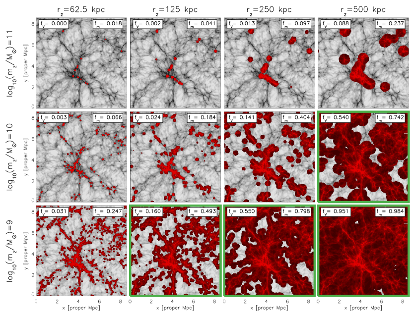
Figure 1: Thin (1 comoving Mpc/$h$ thick) slices of the $z=3$ gas density field through the centre of the L025N512 simulation for models with different $r_{\rm z}$ (the proper radius out to which galaxies enrich the IGM) and $m_{\rm z}$ (the minimum halo mass that is responsible for enriching the IGM). Each density field is shown in grey-scale in regions where, for a given combination of $r_{\rm z}$ and $m_{\rm z}$, the gas is unenriched, and in red where metals are present. Each row of plots corresponds to a different value of $m_{\rm z}$ and each column shows a different value of $r_{\rm z}$. The numbers at the top of each panel show what fraction of the total simulation volume ($f_{\rm V}$) and gas mass ($f_{\rm m}$) are enriched with metals in each model. Panels outlined in green show models that satisfy the constraints provided by the observed $\tau\hbox{\scriptsize C\,{\tiny IV}}-\tau\hbox{\scriptsize H\,{\tiny I}}$ relation. All models that reproduce the observations have volume filling factors $>10\%$.

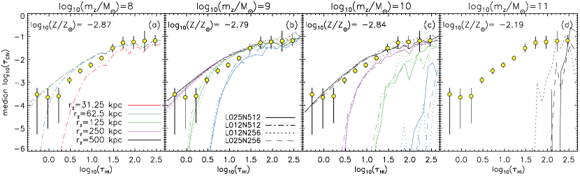
Figure 2: The dependence of the relation between $\tau\hbox{\scriptsize H\,{\tiny I}}$ and $\tau\hbox{\scriptsize C\,{\tiny IV}}$ on the model parameters $r_{\rm z}$ (the physical radius out to which galaxies enrich the IGM) and $m_{\rm z}$ (the minimum halo mass that is capable of enriching the IGM). Each panel shows a different choice for $m_{\rm z}$ and in each of the panels the yellow points with error bars show the observed relation of Aguirre et al. (2005), with arrows representing upper limits. The curves show the simulation results, with the different colours representing the different choices for $r_{\rm z}$, and different line styles corresponding to different simulations. The metallicity, $Z$, required to match the normalisation of the observed data at the maximum value of $\tau\hbox{\scriptsize H\,{\tiny I}}$ (for the maximum value of $r_{\rm z}$) is shown at the top of each panel. The black curve in panel a is not visible because for $m_{\rm z}=10^{8}\,{\rm M}_{\odot}$ both $r_{\rm z}=250$ kpc and $r_{\rm z}=500$ kpc have $f_{\rm V}=1.00$ and hence predict identical results. All coloured curves in each panel are scaled to the same metallicity. In order to match the observed median optical depth of C iv in regions with a low H i optical depth, it is necessary that low-mass haloes ($m_{\rm z}\leq 10^{10.5}\,{\rm M}_{\odot}$) enrich the IGM out to distances $>10^{2}\,$kpc.

Fig. 1 shows a thin (1 comoving Mpc/$h$ thick) slice of the density field at $z=3$ through the centre of the L025N512 simulation. Each panel shows a different combination of $r_{\rm z}$ and $m_{\rm z}$. Gas with zero metallicity is shown in grey-scale, while metal-enriched gas is coloured red. In addition, the values for $f_{\rm V}$ and $f_{\rm m}$ are indicated for each model. Panels showing metal distributions that are consistent with the observations (see below) are outlined in green.

The fractions of the mass and volume that are enriched do not track each other in a simple way. The ratio $f_{\rm m}/f_{\rm V}$ is always $\geq 1$ because metals are only placed around collapsed structures and thus preferentially in overdense regions. For $m_{\rm z}=10^{10}\,{\rm M}_{\odot}$, changing $r_{\rm z}$ from 31.25 kpc to 500 kpc changes the ratio $f_{\rm m}/f_{\rm V}$ from 22.7 to 1.3, as a larger value of $r_{\rm z}$ at fixed $m_{\rm z}$ allows metals to disperse further out of the high-density peaks. Similarly, changing $m_{\rm z}$ at fixed $r_{\rm z}=250$ kpc, we find that the ratio $f_{\rm m}/f_{\rm V}$ rises from 2.8 for $m_{\rm z}=10^{9}\,{\rm M}_{\odot}$ to 7.5 for $m_{\rm z}=10^{11}\,{\rm M}_{\odot}$, because more massive haloes are preferentially located in higher density environments. Given that we understand how changing the pattern of metal enrichment alters the relative mass and volume filling factors, we now ask how this impacts the $\tau\hbox{\scriptsize C\,{\tiny IV}}-\tau\hbox{\scriptsize H\,{\tiny I}}$ relation.

The curves in Fig. 2 show the relation between $\tau\hbox{\scriptsize C\,{\tiny IV}}$ and $\tau\hbox{\scriptsize H\,{\tiny I}}$ in the synthetic absorption spectra. Each panel corresponds to a different $m_{\rm z}$. The solid lines in panels b, c and d ($\log_{10}(m_{\rm z}/{\rm M}_{\odot})={9,10,11}$, respectively) show the predicted $\tau\hbox{\scriptsize C\,{\tiny IV}}-\tau\hbox{\scriptsize H\,{\tiny I}}$ relation from the L025N512 simulation with various imposed metallicity distributions. The dot-dashed lines in panels a and b ($\log_{10}(m_{\rm z}/{\rm M}_{\odot})={8,9}$, respectively) show the predicted $\tau\hbox{\scriptsize C\,{\tiny IV}}-\tau\hbox{\scriptsize H\,{\tiny I}}$ relations for the small volume, high-resolution simulation, L012N512. In every panel we compare our simulated predictions to the observed optical depth pixel statistics of Schaye et al. (2003), for the redshift range $2.479\leq z\leq 4.033$, as published in Aguirre et al. (2005), shown as the yellow points with $1\sigma$ error bars. The data come from six quasar spectra, Q0420–388, Q1425+604, Q2126–158, Q1422+230, Q0055–269, and Q1055+461, that were taken with either the Keck/HIRES or the VLT/UVES. A full description of the sample is given in Schaye et al. (2003). In each panel $Z$ was chosen such that the $r_{\rm z}=500$ kpc curve exactly matches the observations at the highest value of $\tau\hbox{\scriptsize H\,{\tiny I}}$ and the metallicity required for this normalisation is given in each panel.

In the present work we are not aiming to reproduce the shape of the $\tau\hbox{\scriptsize C\,{\tiny IV}}-\tau\hbox{\scriptsize H\,{\tiny I}}$ relation in detail and, indeed, would not necessarily expect our simple models to be capable of doing this. Rather, we require that the models predict a median $\tau\hbox{\scriptsize C\,{\tiny IV}}-\tau\hbox{\scriptsize H\,{\tiny I}}$ relation that is consistent with, or larger, than observed and that the $\tau\hbox{\scriptsize C\,{\tiny IV}}-\tau\hbox{\scriptsize H\,{\tiny I}}$ relation is not steeper than observed. We effectively combine the two conditions by scaling $Z$ in each run to match the normalisation of the observed $\tau\hbox{\scriptsize C\,{\tiny IV}}-\tau\hbox{\scriptsize H\,{\tiny I}}$ relation at $\log_{10}\tau\hbox{\scriptsize H\,{\tiny I}}=2.5$, the largest optical depth probed by the observations, and then requiring the model to predict median $\tau\hbox{\scriptsize C\,{\tiny IV}}$ at low $\tau\hbox{\scriptsize H\,{\tiny I}}$ that are consistent with or greater than observed.

We stress that overprediction of $\tau\hbox{\scriptsize C\,{\tiny IV}}$ is not a problem at small $\tau\hbox{\scriptsize H\,{\tiny I}}$ because our simple models make the assumption that the metallicity inside each enriched bubble is constant with radius. The overestimate at low $\tau\hbox{\scriptsize C\,{\tiny IV}}$ could therefore be solved by imposing a metallicity that decreases with radius. On the other hand, we will assume that underprediction of $\tau\hbox{\scriptsize C\,{\tiny IV}}$ at low $\tau\hbox{\scriptsize H\,{\tiny I}}$ signals the failure of the model because a metallicity that increases with radius is likely unphysical. Such an unphysical metallicity gradient would also have been required if we had chosen to scale the metallicity to match the low $\tau\hbox{\scriptsize H\,{\tiny I}}$ points, because the unsuccessful, constant metallicity models predict much steeper $\tau\hbox{\scriptsize C\,{\tiny IV}}-\tau\hbox{\scriptsize H\,{\tiny I}}$ relations than observed (see Fig. 2). In fact, such an approach would not be possible for most of the models that we rule out, because they typically predict the median $\tau\hbox{\scriptsize C\,{\tiny IV}}$ to be zero at low $\tau\hbox{\scriptsize H\,{\tiny I}}$.

In principle, we could produce significantly better fits to the $\tau\hbox{\scriptsize C\,{\tiny IV}}-\tau\hbox{\scriptsize H\,{\tiny I}}$ relation by considering more complex models (e.g. including metallicity gradients, anisotropic outflows or scatter in metallicities), but that is not the aim of the present study. Given that such models would still not be self-consistent if the enrichment is done in post-processing, it is not obvious that the use of more complex models would be justified.

Before proceeding, we evaluate the effect of our simulation’s finite box size and numerical resolution on our results. Firstly, the dotted curves in panels b, c and d show the effect of decreasing the box size by a factor of two in each dimension, while keeping the numerical resolution fixed (L012N256 vs. L025N512). It is clear that for $m_{\rm z}\leq 10^{10}\,{\rm M}_{\odot}$ our results are converged with respect to box size, but that for $m_{\rm z}=10^{12}\,{\rm M}_{\odot}$ the 12.5 Mpc/$h$ and 25 Mpc/$h$ volumes predict significantly different $\tau\hbox{\scriptsize C\,{\tiny IV}}-\tau\hbox{\scriptsize H\,{\tiny I}}$ relations, indicating that for haloes of this mass the simulation results from the 25 Mpc/$h$ volume are not necessarily converged. Note, however, that allowing only haloes with masses $\geq 10^{11}\,{\rm M}_{\odot}$ to enrich the IGM yields $\tau\hbox{\scriptsize C\,{\tiny IV}}-\tau\hbox{\scriptsize H\,{\tiny I}}$ relations that are far steeper than those allowed by the observations. We thus conclude that our simulation boxes are sufficiently large for our purposes. Secondly, the long-dashed curves in panels c and d show the effect of degrading the simulation mass resolution by a factor of eight while keeping the box size constant (L025N256 vs. L025N512). Decreasing the resolution does not significantly change any of the conclusions derived from this analysis.

Considering first the case where only haloes with mass $>10^{11}\,{\rm M}_{\odot}$ enrich the IGM, we find that even if such objects were able to enrich out to a radius of $500$ kpc, they would fall far short of being able to account for the observed $\tau\hbox{\scriptsize C\,{\tiny IV}}$ at $\tau\hbox{\scriptsize H\,{\tiny I}}<10$ because there are too few of them to enrich enough of the low-density gas. If we now consider a lower value of $m_{\rm z}=10^{9}\,{\rm M}_{\odot}$, the lower clustering strength and higher number density of these less massive haloes allows them to pollute lower density gas, even if they enrich out to much smaller distances. All values of $r_{\rm z}\geq 125$ kpc provide a good match to the observations (note that measurements of $\tau\hbox{\scriptsize C\,{\tiny IV}}$ are upper limits for $\log_{10}(\tau\hbox{\scriptsize H\,{\tiny I}})<0.3$). The intermediate value of $m_{\rm z}=10^{10}\,{\rm M}_{\odot}$ provides, as expected, results that are intermediate between the two cases presented above: the observations are reproduced for $r_{\rm z}=500\,$kpc but not for $r_{\rm z}=250\,$kpc and smaller. Considering now the extremely high-resolution simulation (L012N512; panel a), we find that if $m_{\rm z}$ is as low as $10^{8}\,{\rm M}_{\odot}$, then the observed $\tau\hbox{\scriptsize C\,{\tiny IV}}-\tau\hbox{\scriptsize H\,{\tiny I}}$ relation can be matched even if $r_{\rm z}$ is as small as 62.5 kpc, but not for $r_{\rm z}=$31.25 kpc.

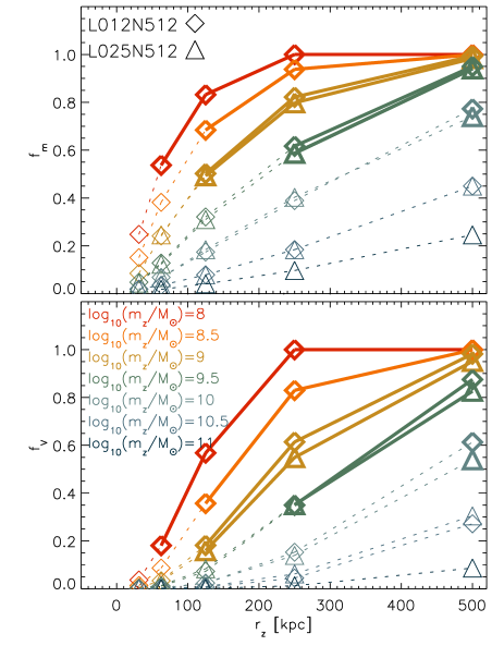
Figure 3: Fraction of the volume ($f_{\rm V}$; top panel) and gas mass ($f_{\rm m}$; bottom panel) of the simulation that is enriched with metals as a function of $r_{\rm z}$ (the proper radius out to which galaxies enrich the IGM). Each colour represents a different choice for $m_{\rm z}$ (the minimum halo mass that is capable of enriching the IGM), and the diamonds (triangles) show results for L012N512 (L025N512). Thick curves and symbols show models that reproduce the $\tau\hbox{\scriptsize C\,{\tiny IV}}-\tau\hbox{\scriptsize H\,{\tiny I}}$ relation, thin, dotted lines show models that do not. We require $f_{\rm V}>0.1$ and $f_{\rm m}>0.5$ in order to match the observations.

Our results for the volume and mass filling factors of metals are summarised in Fig. 3, where we show the mass (upper panel) and volume (lower panel) filling fractions as a function of $r_{\rm z}$ for different values of $m_{\rm z}$. Models that predict enough C iv at low $\tau\hbox{\scriptsize H\,{\tiny I}}$ are indicated with bold symbols and are connected with solid, thick lines. It is clear that in order to reproduce the observations, we require that the IGM is enriched primarily by low-mass ($m_{\rm tot}<10^{10}\,{\rm M}_{\odot}$) haloes that are capable of driving gas out to distances $>10^{2}\,$kpc by $z=3$. Allowing only haloes with masses $\geq 10^{10.5}\,{\rm M}_{\odot}$ to enrich the IGM, results in metal distributions that fall far short of the observations for all sensible values of $r_{\rm z}$. Models relying on (the progenitors of) observed Lyman break galaxies ($m_{\rm tot}\sim 10^{12}\,{\rm M}_{\odot}$; Adelberger et al., 2005) to do the enrichment, predict filling factors that are far too small to account for the observations and have not even been plotted. In our models, the volume filling factor of metals must be $>10\%$ in order to reproduce the observations, indicating that the observed $\tau\hbox{\scriptsize C\,{\tiny IV}}-\tau\hbox{\scriptsize H\,{\tiny I}}$ relation tells us robustly that a significant fraction of the volume and mass of the IGM is enriched by metals. On the other hand, a model volume filling factor $>10\%$ is not necessarily sufficient. Models that attain such large volume fractions by enriching the gas around high-mass haloes to very large distances often fail to reproduce the observations. We note that the values of the volume and mass filling fractions that we infer by comparing our models to the observations are approximate, even ignoring uncertainties associated with small-scale metal mixing. The filling fractions could change by factors of a few due to, for example, scatter in the metallicity around galaxies of a fixed mass and non-spherical bubbles.

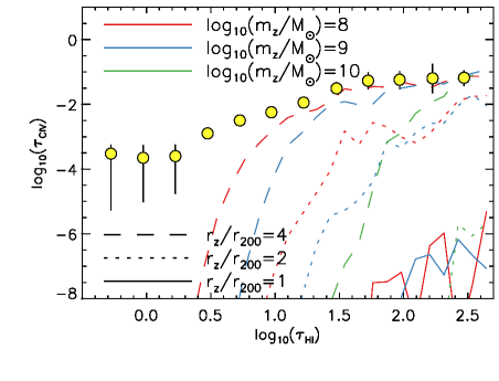
Figure 4: The $z=3$ $\tau\hbox{\scriptsize C\,{\tiny IV}}-\tau\hbox{\scriptsize H\,{\tiny I}}$ relation for models in which $r_{\rm z}$ (the physical radius out to which galaxies enrich the IGM) is set to a fixed multiple of the halo virial radius. Yellow points with error bars represent the observations presented in Aguirre et al. (2005). Each curve represents a different imposed metal enrichment pattern, with different colours corresponding to different values of $m_{\rm z}$, and different line styles representing different choices for $r_{\rm z}$, as indicated in the legends. Even if all haloes can enrich the IGM out to four times their own virial radius, the observed $\tau\hbox{\scriptsize C\,{\tiny IV}}-\tau\hbox{\scriptsize H\,{\tiny I}}$ relation is not reproduced. This implies that dynamical effects alone are insufficient to explain the observed distribution of C iv.

Finally, in Fig. 4 we show the effect of allowing haloes to enrich out a fixed multiple of their virial radii, $r_{200}$. The yellow data points with error bars show again the observations of Schaye et al. (2003) as presented in Aguirre et al. (2005), and the curves show the results for the imposed metallicity distributions indicated in the legend. It is striking that even if all haloes that form stars are able to pollute the IGM as far out as four times their own virial radius, the low optical depth part of the $\tau\hbox{\scriptsize C\,{\tiny IV}}-\tau\hbox{\scriptsize H\,{\tiny I}}$ relation is not reproduced. As dynamical processes (e.g. tidal or ram pressure stripping) are only expected to affect the metal distribution on scales $\la r_{200}$, this implies that some sort of ejective feedback is necessary in order to pollute the low-density IGM. The conclusion that dynamical processes such as stripping are not, on their own, sufficient is consistent with the models of Aguirre et al. (2001a) as well as with the hydrodynamical simulations of Wiersma et al. (2011).

4 Discussion and conclusions

By combining realistic cosmological density and temperature distributions with toy models for the metal distribution, in which only haloes more massive than a critical mass ($m_{\rm z}$) are able to enrich a spherical region (of proper radius $r_{\rm z}$) to a metallicity of $Z$, we have investigated which metal distributions can reproduce the observations of C iv associated with weak H i absorption ($\tau_{\rm HI}\ll 10$) as measured in quasar absorption spectra.

The results presented in Sec. 3 imply that in order to match the observed median optical depth of C iv as a function of $\tau_{\rm HI}$, we require that low-mass haloes, $m_{200}<10^{10}\,{\rm M}_{\odot}$, are able to drive metals into the IGM, enriching the gas around them out to proper distances of $\ga 10^{2}$ kpc to metallicities of $\sim 10^{-3}\,{\rm Z}_{\odot}$.

We now verify that this scenario is physically possible by comparing the required metal mass to an estimate of the maximum allowed mass of carbon in the Universe. We can estimate the maximum allowed mass of carbon in the IGM from the stellar mass density at $z=3$. Under the assumption that all of the stars formed in a single burst at $t=0$, and assuming a Chabrier stellar initial mass function and using the lifetimes, yields and supernova rates used in the simulation and summarised in Wiersma et al. (2009b), the maximum allowed cosmic density of carbon is $0.006\rho_{\ast}$, where $\rho_{\ast}$ is the cosmic density in stars and has been measured to be $\rho_{\ast}=10^{7.55}\,{\rm M}_{\odot}/{\rm Mpc}^{3}$ (Marchesini et al., 2009) at $z=3$, giving us a maximum allowed total density in carbon of $\rho_{{\rm C}}=2.2\times 10^{5}\,{\rm M}_{\odot}/{\rm Mpc}^{3}$. For the models that can successfully reproduce the observed optical depth distributions, the cosmic density of carbon varies from $8\times 10^{3}\,{\rm M}_{\odot}/{\rm Mpc}^{3}$ ($m_{\rm z}=10^{10}\,{\rm M}_{\odot}$; $r_{\rm z}=250\,{\rm kpc}$) to $2\times 10^{4}\,{\rm M}_{\odot}/{\rm Mpc}^{3}$ ($m_{\rm z}=10^{9}\,{\rm M}_{\odot}$; $r_{\rm z}=500\,{\rm kpc}$). In each case the total amount of carbon is an order of magnitude below the maximum allowed amount, so the models are physically reasonable on these grounds.

We thus conclude that in order to recover the observed median C iv optical depth in regions of low H i optical depth ($\tau\hbox{\scriptsize H\,{\tiny I}}\sim 1-10$), we require that the galaxies in low-mass haloes ($m_{\rm z}<10^{10}\,{\rm M}_{\odot}$) enrich the IGM out to distances $\ga 10^{2}\,$kpc. Galaxies residing in much higher mass haloes ($m_{\rm z}>10^{10.5}\,{\rm M}_{\odot}$) are too rare and too strongly clustered to contribute significantly to the enrichment of the low-density IGM. In every one of the models that is capable of reproducing the observations, the metal volume filling factor is $>10\%$ and the gas mass fraction enriched with metals is $>50\%$.

As discussed in detail in section 2.2, our models are not fully self-consistent in the sense that we have imposed metal distribution is post-processing. Although we found that post-processing hydro simulations without winds or with very strong winds led to identical conclusions, we cannot rule out the possitibity that future self-consistent models would yield different results. Unfortunately, current simulations suffer from large uncertainties due to their use of subgrid recipes for the generation of winds and still lack the resolution to resolve outflows from low-mass galaxies in a representative volume.

Two additional caveats must, however, be stressed. Firstly, the models presented here implicitly assume that the metals are well mixed on small scales. If, as suggested by observations (e.g. Schaye et al., 2007), the intergalactic metals are concentrated in metal-rich patches which together account for large covering factors, then the required filling factors could be smaller. In that case the filling factors derived here apply to the metal distribution smoothed over the scales that are somewhat smaller than the size of the bubbles, i.e. tens of kpc.

Secondly, there exists considerable uncertainty in the spectral shape of the ionizing background, which leads to uncertainties the fraction of carbon that exists as C iv. Aguirre et al. (2008) considered several models for the UV background, including some extreme ones, and found that only the fiducial Haardt & Madau (2001) model, which is the model used here, resulted in reasonable values for the relative abundances inferred from observations. Schaye et al. (2003) found that assuming a much harder (softer) spectrum would flatten (steepen) the metallicity-density relation inferred from the observed $\tau\hbox{\scriptsize C\,{\tiny IV}}$-$\tau\hbox{\scriptsize H\,{\tiny I}}$ relation, which implies that our models would predict steeper (flatter) $\tau\hbox{\scriptsize C\,{\tiny IV}}$-$\tau\hbox{\scriptsize H\,{\tiny I}}$ relations than for our standard UV background, which would increase (decrease) the inferred filling factors.

Our finding that the observations imply that the IGM was enriched by very low-mass galaxies is in agreement with a variety of theoretical studies (e.g. Aguirre et al., 2001b; Madau et al., 2001; Scannapieco et al., 2002; Thacker et al., 2002; Samui et al., 2008; Oppenheimer et al., 2009; Wiersma et al., 2010). For example, by modelling the propagation of galactic winds in already completed simulations, Aguirre et al. (2001b) found that in order to explain the metallicities measured in the low column density part of the IGM, galaxies with baryonic masses $>10^{8.5}\,{\rm M}_{\odot}$ needed to launch winds with velocities of at least $200-300$ km/s. The results presented here are also consistent with Wiersma et al. (2010), who used fully self-consistent hydrodynamical simulations (including the simulations underlying our models) that massive haloes ($>10^{12}\,{\rm M}_{\odot}$) are unimportant for the enrichment of the diffuse IGM and that most of the metals that reside in the IGM at $z=0$ were ejected by a population of low-mass galaxies at high redshift.

In contrast, Scannapieco et al. (2006) found that in order to match the strong clustering of C iv lines that they measured in their observations, the absorption needed to be generated primarily by gas that is strongly clustered around massive galaxies. Their best fit model required $m_{\rm z}=10^{12}\,{\rm M}_{\odot}$ and $r_{\rm z}=500\,{\rm kpc}$. Using these parameters in our model leads to such low volume ($f_{\rm V}=6\times 10^{-3}$) and mass ($f_{\rm m}=0.03$) filling factors that the corresponding curves would not appear on any of the plots presented here. We plan to explore the apparent tension between line clustering and optical depth statistics in future work.

In summary, we have found that in order for a simulated cosmological gas density field to reproduce the observed $\tau\hbox{\scriptsize C\,{\tiny IV}}-\tau\hbox{\scriptsize H\,{\tiny I}}$ relation, we require that both the fractions of the volume and mass of the IGM that have been polluted with metals are substantial, with all our successful parameter choices yielding model volume filling factors greater than 10% and model mass filling factors greater than 50%. The models favour metals being ejected from a population of low-mass ($m_{\rm tot}<10^{10}\,{\rm M}_{\odot}$) haloes at high redshift.

References

- Adelberger et al. (2005) Adelberger K. L., Steidel C. C., Pettini M., Shapley A. E., Reddy N. A., Erb D. K., 2005, ApJ, 619, 697
- Aguirre et al. (2008) Aguirre A., Dow-Hygelund C., Schaye J., Theuns T., 2008, ApJ, 689, 851
- Aguirre et al. (2001a) Aguirre A., Hernquist L., Schaye J., Katz N., Weinberg D. H., Gardner J., 2001a, ApJ, 561, 521
- Aguirre et al. (2001b) Aguirre A., Hernquist L., Schaye J., Weinberg D. H., Katz N., Gardner J., 2001b, ApJ, 560, 599
- Aguirre et al. (2005) Aguirre A., Schaye J., Hernquist L., Kay S., Springel V., Theuns T., 2005, ApJL, 620, L13
- Aracil et al. (2004) Aracil B., Petitjean P., Pichon C., Bergeron J., 2004, A&A, 419, 811
- Bertone et al. (2005) Bertone S., Stoehr F., White S. D. M., 2005, MNRAS, 359, 1201
- Carswell et al. (2002) Carswell B., Schaye J., Kim T., 2002, ApJ, 578, 43
- Cen & Chisari (2011) Cen R., Chisari N. E., 2011, ApJ, 731, 11
- Cen et al. (2005) Cen R., Nagamine K., Ostriker J. P., 2005, ApJ, 635, 86
- Cen & Ostriker (2006) Cen R., Ostriker J. P., 2006, ApJ, 650, 560
- Cowie et al. (1995) Cowie L. L., Hu E. M., Songaila A., 1995, AJ, 110, 1576
- Cowie & Songaila (1998) Cowie L. L., Songaila A., 1998, Nature, 394, 44
- Dalla Vecchia & Schaye (2008) Dalla Vecchia C., Schaye J., 2008, MNRAS, 387, 1431
- Efstathiou (1992) Efstathiou G., 1992, MNRAS, 256, 43P
- Ellison et al. (2000) Ellison S. L., Songaila A., Schaye J., Pettini M., 2000, AJ, 120, 1175
- Faucher-Giguère et al. (2008) Faucher-Giguère C., Lidz A., Hernquist L., Zaldarriaga M., 2008, ApJ, 688, 85
- Ferland et al. (1998) Ferland G. J., Korista K. T., Verner D. A., Ferguson J. W., Kingdon J. B., Verner E. M., 1998, PASP, 110, 761
- Germain et al. (2009) Germain J., Barai P., Martel H., 2009, ApJ, 704, 1002
- Haardt & Madau (2001) Haardt F., Madau P., 2001, in Clusters of Galaxies and the High Redshift Universe Observed in X-rays, D. M. Neumann & J. T. V. Tran, ed.
- Kobayashi et al. (2007) Kobayashi C., Springel V., White S. D. M., 2007, MNRAS, 376, 1465
- Madau et al. (2001) Madau P., Ferrara A., Rees M. J., 2001, ApJ, 555, 92
- Marchesini et al. (2009) Marchesini D., van Dokkum P. G., Förster Schreiber N. M., Franx M., Labbé I., Wuyts S., 2009, ApJ, 701, 1765
- Martin (2005) Martin C. L., 2005, ApJ, 621, 227
- Oppenheimer & Davé (2006) Oppenheimer B. D., Davé R., 2006, MNRAS, 373, 1265
- Oppenheimer & Davé (2008) —, 2008, MNRAS, 387, 577
- Oppenheimer et al. (2009) Oppenheimer B. D., Davé R., Finlator K., 2009, MNRAS, 396, 729
- Pettini et al. (2001) Pettini M., Shapley A. E., Steidel C. C., Cuby J., Dickinson M., Moorwood A. F. M., Adelberger K. L., Giavalisco M., 2001, ApJ, 554, 981
- Pieri et al. (2010) Pieri M. M., Frank S., Weinberg D. H., Mathur S., York D. G., 2010, ApJL, 724, L69
- Pieri & Haehnelt (2004) Pieri M. M., Haehnelt M. G., 2004, MNRAS, 347, 985
- Pieri et al. (2007) Pieri M. M., Martel H., Grenon C., 2007, ApJ, 658, 36
- Pinsonneault et al. (2010) Pinsonneault S., Martel H., Pieri M. M., 2010, ApJ, 725, 2087
- Quinn et al. (1996) Quinn T., Katz N., Efstathiou G., 1996, MNRAS, 278, L49
- Rakic et al. (2011) Rakic O., Schaye J., Steidel C. C., Rudie G. C., 2011, MNRAS, 414, 3265
- Rauch et al. (1997) Rauch M., Miralda-Escude J., Sargent W. L. W., Barlow T. A., Weinberg D. H., Hernquist L., Katz N., Cen R., Ostriker J. P., 1997, ApJ, 489, 7
- Samui et al. (2008) Samui S., Subramanian K., Srianand R., 2008, MNRAS, 385, 783
- Scannapieco et al. (2002) Scannapieco E., Ferrara A., Madau P., 2002, ApJ, 574, 590
- Scannapieco et al. (2006) Scannapieco E., Pichon C., Aracil B., Petitjean P., Thacker R. J., Pogosyan D., Bergeron J., Couchman H. M. P., 2006, MNRAS, 365, 615
- Schaye (2001) Schaye J., 2001, ApJ, 559, 507
- Schaye & Aguirre (2005) Schaye J., Aguirre A., 2005, in IAU Symposium, Vol. 228, From Lithium to Uranium: Elemental Tracers of Early Cosmic Evolution, V. Hill, P. François, & F. Primas, ed., pp. 557–568
- Schaye et al. (2003) Schaye J., Aguirre A., Kim T., Theuns T., Rauch M., Sargent W. L. W., 2003, ApJ, 596, 768
- Schaye et al. (2007) Schaye J., Carswell R. F., Kim T., 2007, MNRAS, 379, 1169
- Schaye & Dalla Vecchia (2008) Schaye J., Dalla Vecchia C., 2008, MNRAS, 383, 1210
- Schaye et al. (2010) Schaye J., Dalla Vecchia C., Booth C. M., Wiersma R. P. C., Theuns T., Haas M. R., Bertone S., Duffy A. R., McCarthy I. G., van de Voort F., 2010, MNRAS, 402, 1536
- Schaye et al. (2000a) Schaye J., Rauch M., Sargent W. L. W., Kim T., 2000a, ApJL, 541, L1
- Schaye et al. (2000b) Schaye J., Theuns T., Rauch M., Efstathiou G., Sargent W. L. W., 2000b, MNRAS, 318, 817
- Schwartz & Martin (2004) Schwartz C. M., Martin C. L., 2004, ApJ, 610, 201
- Shapley et al. (2003) Shapley A. E., Steidel C. C., Pettini M., Adelberger K. L., 2003, ApJ, 588, 65
- Shen et al. (2010) Shen S., Wadsley J., Stinson G., 2010, MNRAS, 407, 1581
- Simcoe et al. (2004) Simcoe R. A., Sargent W. L. W., Rauch M., 2004, ApJ, 606, 92
- Songaila (2005) Songaila A., 2005, AJ, 130, 1996
- Spergel et al. (2007) Spergel D. N., Bean R., Doré O., et al., 2007, ApJS, 170, 377
- Springel (2005) Springel V., 2005, MNRAS, 364, 1105
- Springel et al. (2001) Springel V., White S. D. M., Tormen G., Kauffmann G., 2001, MNRAS, 328, 726
- Steidel et al. (2010) Steidel C. C., Erb D. K., Shapley A. E., Pettini M., Reddy N., Bogosavljević M., Rudie G. C., Rakic O., 2010, ApJ, 717, 289
- Tescari et al. (2011) Tescari E., Viel M., D’Odorico V., Cristiani S., Calura F., Borgani S., Tornatore L., 2011, MNRAS, 411, 826
- Thacker et al. (2002) Thacker R. J., Scannapieco E., Davis M., 2002, ApJ, 581, 836
- Theuns et al. (1998) Theuns T., Leonard A., Efstathiou G., Pearce F. R., Thomas P. A., 1998, MNRAS, 301, 478
- Theuns et al. (2002) Theuns T., Viel M., Kay S., Schaye J., Carswell R. F., Tzanavaris P., 2002, ApJL, 578, L5
- Thoul & Weinberg (1996) Thoul A. A., Weinberg D. H., 1996, ApJ, 465, 608
- Tornatore et al. (2010) Tornatore L., Borgani S., Viel M., Springel V., 2010, MNRAS, 402, 1911
- Tytler et al. (1995) Tytler D., Fan X., Burles S., Cottrell L., Davis C., Kirkman D., Zuo L., 1995, in QSO Absorption Lines, G. Meylan, ed., pp. 289–+
- Weinberg et al. (1997) Weinberg D. H., Miralda-Escude J., Hernquist L., Katz N., 1997, ApJ, 490, 564
- Wiersma et al. (2010) Wiersma R. P. C., Schaye J., Dalla Vecchia C., Booth C. M., Theuns T., Aguirre A., 2010, MNRAS, 409, 132
- Wiersma et al. (2009a) Wiersma R. P. C., Schaye J., Smith B. D., 2009a, MNRAS, 393, 99
- Wiersma et al. (2011) Wiersma R. P. C., Schaye J., Theuns T., 2011, MNRAS, 415, 353
- Wiersma et al. (2009b) Wiersma R. P. C., Schaye J., Theuns T., Dalla Vecchia C., Tornatore L., 2009b, MNRAS, 399, 574