Earthquakes Patterns Statistical properties of signals and noise

Earthquake-like patterns of acoustic emission
in crumpled plastic sheets

Abstract

We report remarkable similarities in the output signal of two distinct out-of-equilibrium physical systems - earthquakes and the intermittent acoustic noise emitted by crumpled plastic sheets - Biaxially Oriented Polypropylene (BOPP) films. We show that both signals share several statistical properties including the distribution of energy, distribution of energy increments for distinct time scales, distribution of return intervals and correlations in the magnitude and sign of energy increments. This analogy is consistent with the concept of universality in complex systems and could provide some insight on the mechanisms behind the complex behavior of earthquakes.

Understanding the underlying mechanisms that govern the complex spatio-temporal behavior of earthquakes is a stimulating challenge[1, 2]. Concepts and methods from statistical physics has been largely applied to study earthquakes, contributing to identify several patterns in seismic activity[3, 4, 5, 6, 7, 8, 9, 10, 11]. This approach also has been contributing to identify universal behavior in earthquakes - similarities between seismic records and the output signal of systems in different research areas.

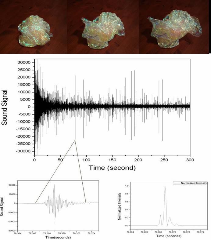
Figure 1: Obtaining the energy intensity from the recorded acoustic noise. Top: A sample of crumpled plastic sheet in relaxation. Middle: The corresponding acoustic noise recorded (in arbitrary units). Bottom-left: Detail of a single event; and Bottom-right: the corresponding intensity of a single event, $I=cp^{2}$, where $c$ is a constant and $p$ is the sound pressure. The variable $S$, given by the area under the corresponding set of peaks, is related to the energy dissipated in the event. Because of the short time distance between events in the beginning of the relaxing process, it was not possible to discriminate individual events. Then, for each experimental dataset, we cut out the first 10 seconds in the recording.

For example, it has been reported that $\gamma$-ray events emitted by neutron stars and earthquakes share several distinctive statistical properties indicating tectonic activity on neutron stars - ’starquakes’ - analogous to earthquakes on Earth[12]. Another example is a reported analogy between earthquakes and the Internet. Specifically, it has been found that two known empirical power laws for earthquakes - the Omori law and the Gutenberg-Richter law - hold also for the Internet (ping experiment). In this context, sudden drastic changes of the Internet time series are referred as ’internetquakes’[13, 14]. Earthquake patterns also can be observed in financial markets. It has been reported, for instance, that stock price fluctuations follow a power law distribution with exponent $\approx 3$[15]. This behavior is quantitatively similar to those found in earthquakes (see refs. [13, 8]), indicating an analogy between natural and financial earthquakes. For other examples of universal behavior in complex systems, see refs. [16, 17, 18, 19, 20, 21].

Here, we compare earthquakes with the output signal of an out-of-equilibrium physical system - the intermittent acoustic noise emitted by crumpled plastic sheets. Some out-of-equilibrium physical systems emit crackling noises as a response to external conditions through events spanning a broad range of sizes[22, 23, 24, 25, 26, 27, 28, 29]. In particular, the sharp and intermittent noises emitted by some kinds of crumpled papers and similar materials - including plastic sheets - qualitatively remember earthquakes which arise when two tectonic plates rub each other. Starting from this qualitative picture, we search for a quantitative support for this analogy. Specifically, in a series of experiments we measure the acoustic noise emitted by a crumpled plastic sheet - a Biaxially Oriented Polypropylene (BOPP) film - in relaxation and compare these records with real data on the magnitude of earthquakes. We find that both processes exhibit several similar statistical properties.

To quantitatively test this analogy, we consider real data on earthquakes obtained from the Northern California catalog for the period 1966-2006[30]. This seismic database contains $\sim 435,000$ records from one of the most active and studied geological faults on the Earth - the San Andreas Fault. For each event, we calculate a measure of the energy dissipated, $E=\exp(M)$, where $M$ is the reported magnitude of the earthquake.

We also perform a series of experiments in order to obtain measures of the energy dissipated by crumpled plastic sheets in relaxation process. First we crumpled a given sample of plastic sheet (of size $1.0m$ x $1.5m$) into a compact ball. This procedure is similar to the common experience of crumpling an unwanted sheet of paper prior to disposing of it[24]. In such conditions, the plastic sheet emit sound in discrete pulses of a variety of intensities for a relatively large time after released to relax (about 10 minutes).

We record the sound emitted with a condenser microphone (Shure Microflex $MX202W/N$) positioned at 1 meter from the sample for five minutes and digitalized at frequency 8000 Hz. For the analysis, the noise was reduced by applying a cutoff filter for low frequencies. A single event is identified by a set of peaks with intensity larger than a threshold value. The start time of the single sound is taken as the time corresponding to the first sound with intensity larger than the threshold, whose value was chosen above the noise intensity. The end time corresponding to the time when the intensity becomes lower than the threshold for a time bigger than a given $t_{c}\approx 1-2ms$ (the characteristic length of single event). Figure 1 shows a typical example of the acoustic emission recorded and the corresponding energy intensity $S$ obtained for a specific event.

We first determine the probability distribution of the energy intensity for earthquakes and crumpled plastic sheets. Figure 2a shows that both distributions are consistent with a power law decay,

$$P(x)\sim x^{-\alpha},$$ (1)

with $\alpha\simeq 3$. This result, already known for earthquakes, suggests that both systems are self-organized into a scale-free state - there is not a typical scale for the dissipated energy. Observe that the power law exponent is quantitatively similar for earthquakes and crumpled plastic sheets.

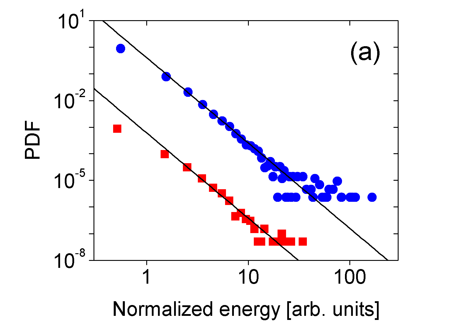
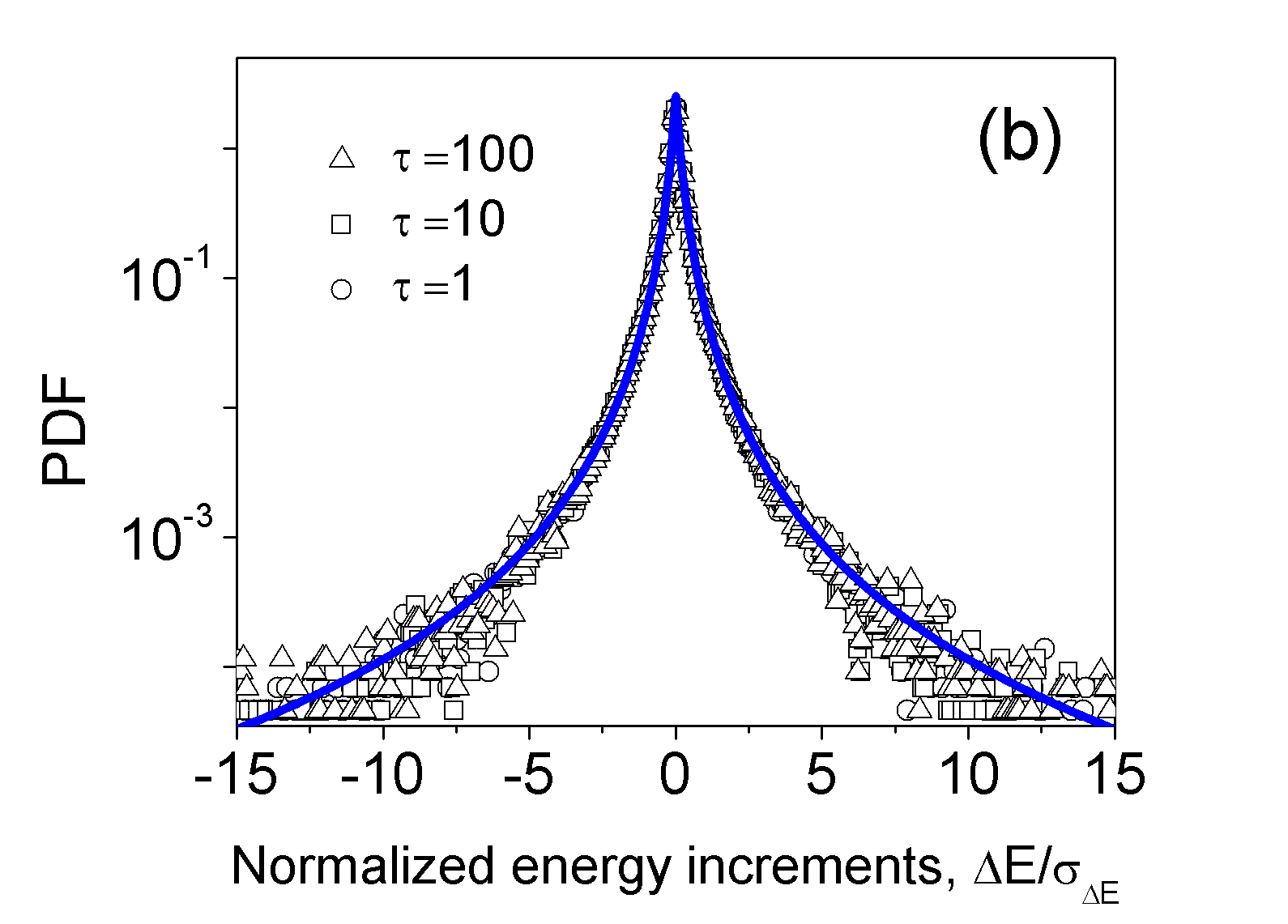
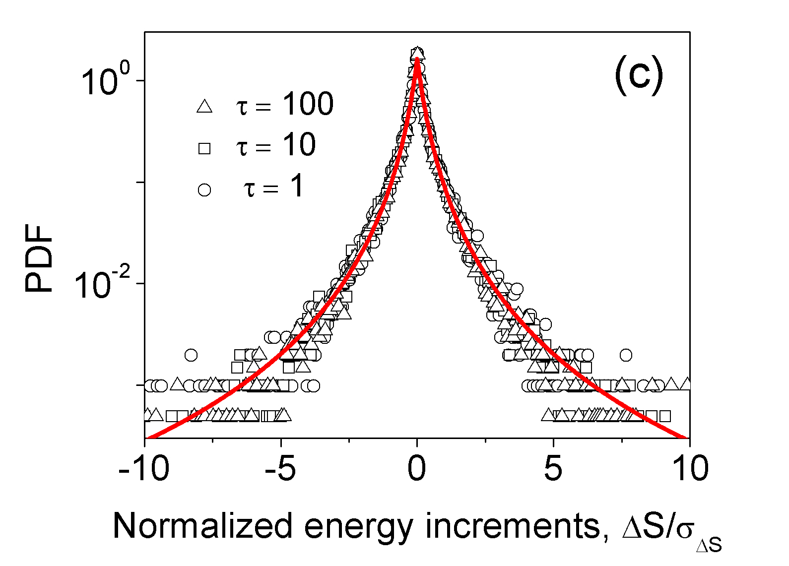
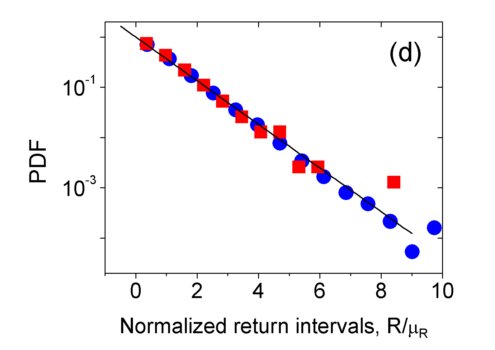
Figure 2: Analysis of the probability density function (PDF) of data. (a) Probability density, $P(E/\sigma_{E})$ and $P(S/\sigma_{S})$, of normalized energy for earthquakes (circles) and crumpled films (squares). $\sigma$ is the standard deviation calculated over all records in a given series. The curves are shown vertically shifted for clarity. The solid lines are power laws given by eq. (1), with exponent $\alpha=3.2$. (b) Probability density of normalized increments, $P(\Delta E/\sigma_{\Delta E})$, for time scales $\tau=1,10,100$. The solid line corresponds to equation (2) with $\alpha=3.2$. (c) Probability density $P(\Delta S/\sigma_{\Delta S})$, for time scales $\tau=1,10,100$. As well as in b, the solid line is given by equation (2) with $\alpha=3.2$. (d) Probability density of normalized return intervals, $P(R/\mu_{R})$, for earthquakes (circles) and crumpled films (squares). In both cases, $R$ is calculated within subseries of size 1016. $\mu_{R}$ is the average of $R$ in a given subseries. The threshold is $R_{c}=2$. The solid line is an exponential distribution $P(r)=\exp[-r]$.

To find information on the dynamics of energy dissipation, we define energy increments as $\Delta E=E(i+\tau)-E(i)$ and $\Delta S=S(i+\tau)-S(i)$, where $E(i)$ and $S(i)$ are proportional to the energy of i-th event. The distributions of energy increments, for different values of the time scale $\tau$, are shown in Figures 2b (earthquakes) and 2c (crumpled plastic sheets). All curves are symmetrical, very peaked and have wings larger than expected for a normal process. In both cases, data for distinct time scales collapse onto a single curve indicating that the distribution of energy increments exhibits a common functional form for all time scales in the range considered. We also shuffled the original series and then calculated the distribution of $\Delta E$ and $\Delta S$ again, but no significant changes were observed. This result may indicate no correlations or weak correlations in the time organization of energy intensities.

Assuming a given variable $x$ following a power law distribution with exponent $\alpha$ (see eq. (1)) and no correlation between two events (a first approximation), the probability distribution for the increments $\Delta x=x(i+\tau)-x(i)$ is given by $P(\Delta x)=K\int_{0}^{\infty}dx\int_{0}^{\infty}dx^{\prime}(xx^{\prime})^{\alpha}\delta(x^{\prime}-x-\epsilon)=K\int_{\tau}^{\infty}dx[x(x+|\epsilon|)]^{-\alpha}$, where $K$ is a normalization constant and $\epsilon$ is a small positive value to avoid divergence in $x=0$. The integration leads, for real and positive $\alpha$, to the normalized probability density function (PDF)

$$P(\Delta x)=\frac{(\alpha-1)^{2}}{\epsilon(2\alpha-1)}F_{1}^{2}\left(\alpha,2\alpha-1,2\alpha,-\frac{|\Delta x|}{\epsilon}\right),$$ (2)

where $F_{1}^{2}$ is the confluent hypergeometric function[8]. This PDF is shown in Figures 2b and 2c in comparison with real data. Notice that both curves are given by eq. (2) with the same parameters. The good adjustment to the data indicates that the distribution of energy increments exhibits a common shape for both systems.

The non-Gaussian behavior of the distributions of energy increments, shown in Figures 2b and 2c, also can be characterized by q-Gaussian distributions - typical in Tsallis statistics[31, 32, 33]. In fact, it has been reported that eq. (2) can be very well reproduced by means of q-Gaussians, whose values of $q$ are related with the parameter $\alpha$[8]. In the range considered, a q-Gaussian distribution, with $q\simeq 1.75$, practically coincides with the curves shown in Figures 2b and 2c (solid lines). For $q>1$, the tails of a q-Gaussian decreases as a power law with exponent $\beta=2/(q-1)$. This result indicates that the tails of the distribution of energy increments follows a power law behavior,

$$P(\Delta x)\sim\Delta x^{-\beta},$$ (3)

with $\beta\simeq 2.7$ for both systems.

Another way to characterize the dynamics of the output signal of a given system is to analyze the return interval series. The return intervals $R$ are defined as the interval between events that exceed a certain threshold $R_{c}$. We obtain $R$ from the normalized energy series - with elements $E/\sigma_{E}$ and $S/\sigma_{S}$, where $\sigma$ is the standard deviation. Figure 2d shows the distribution $P(r)$ for earthquakes and crumpled plastic sheets, where $r=R/\mu_{R}$ and $\mu_{R}$ is the average of $R$ in a given subseries of size 1016 (the typical size of a given experimental record for a crumpled sheet). For comparison, we also show the exponential distribution $P(r)=\exp[-r]$. Observe that the distribution of return intervals for earthquakes and crumpled films share a common shape. We perform a parallel analysis for several values of the threshold $R_{c}$ but no significative changes were observed. The exponential behavior found in the distribution of return intervals suggests no correlation or weak correlations in the energy series of both systems.

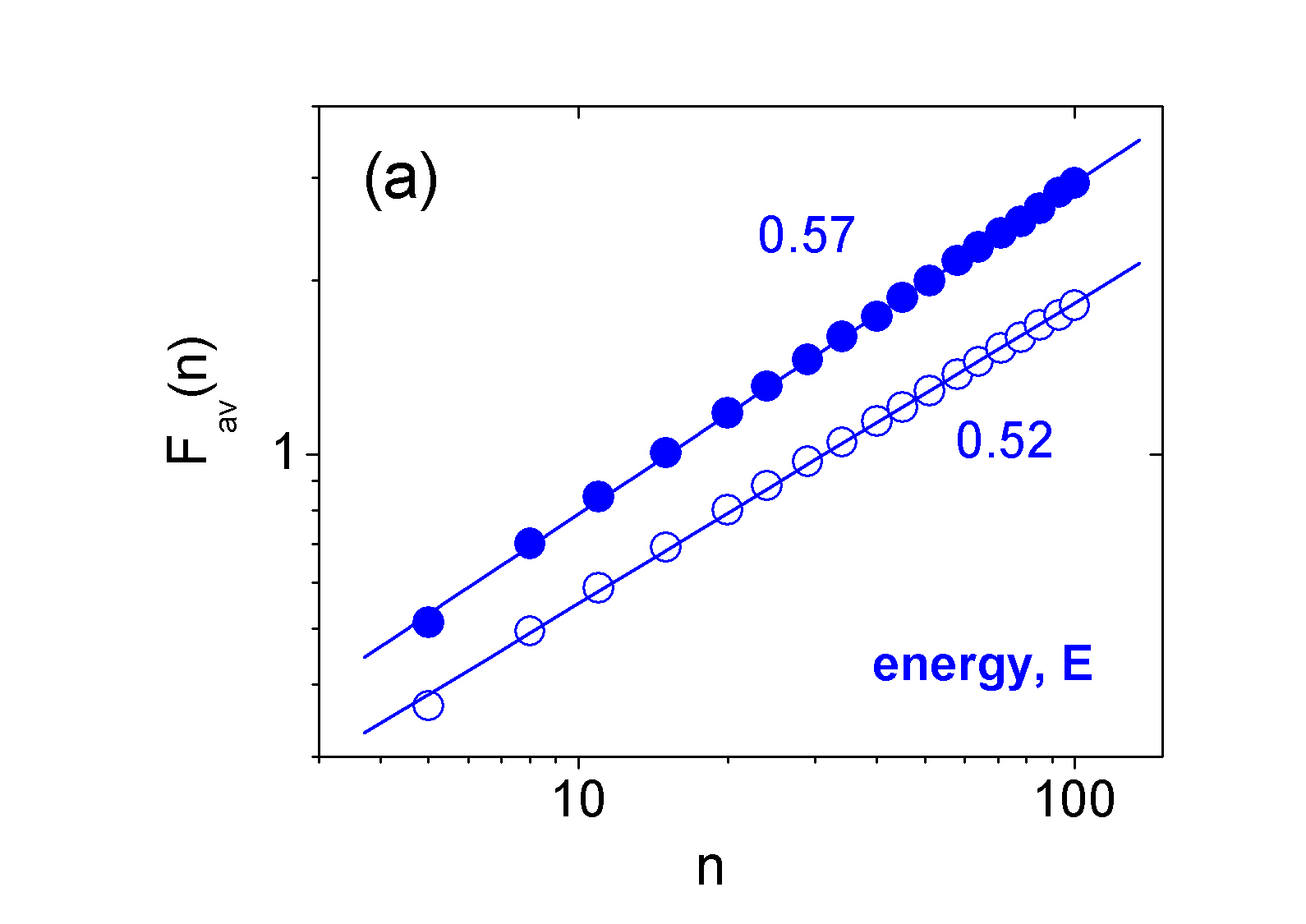
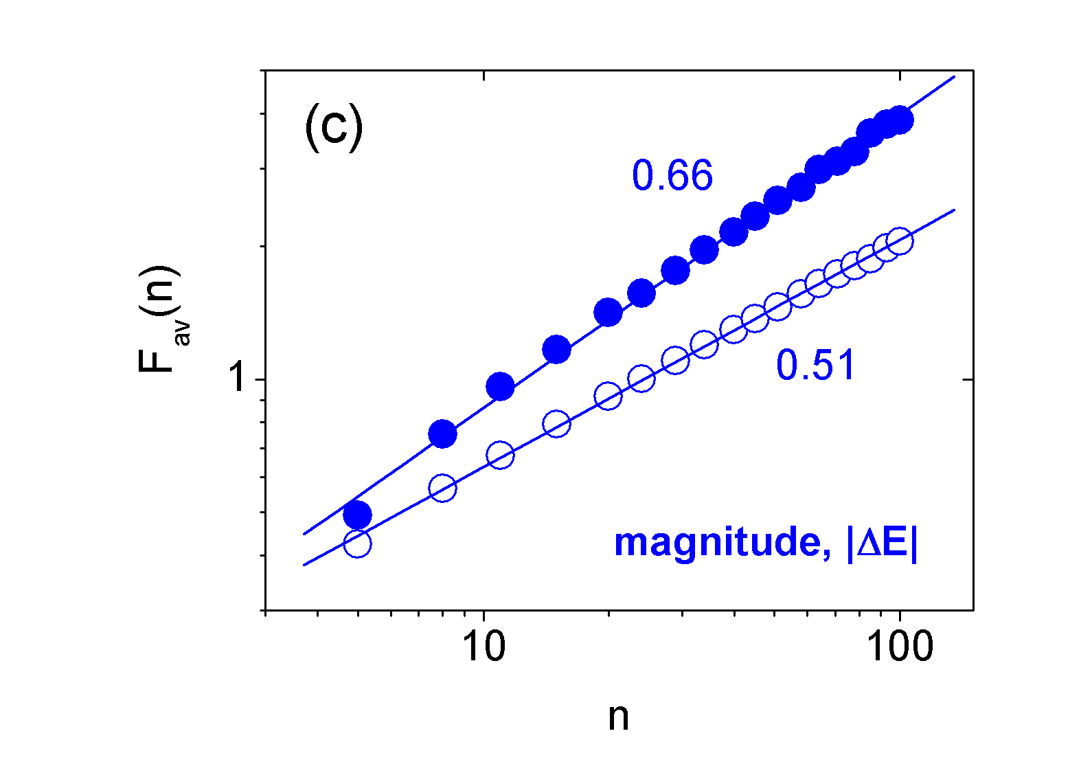
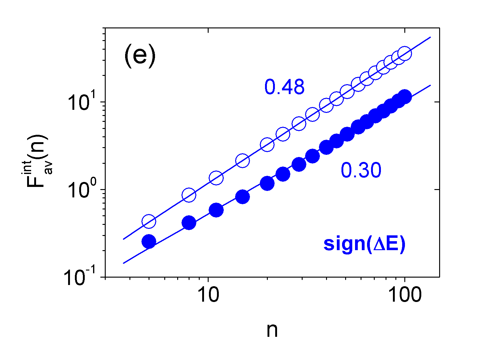
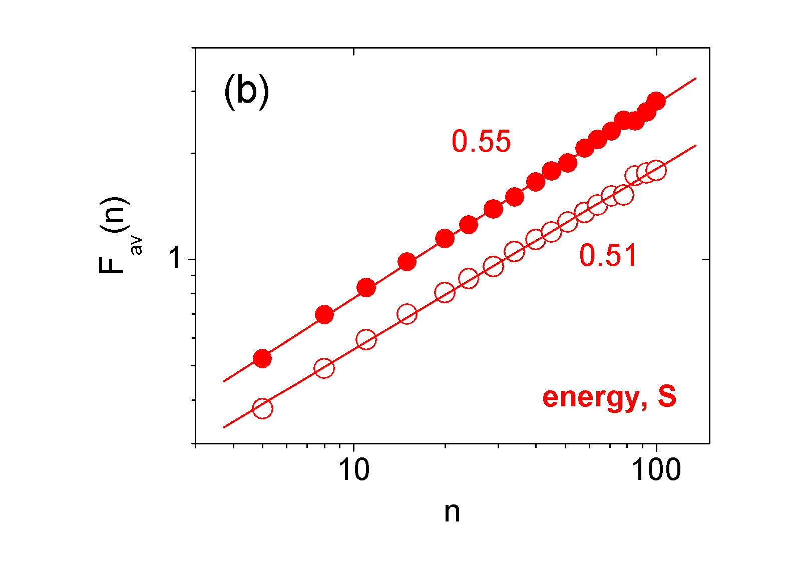
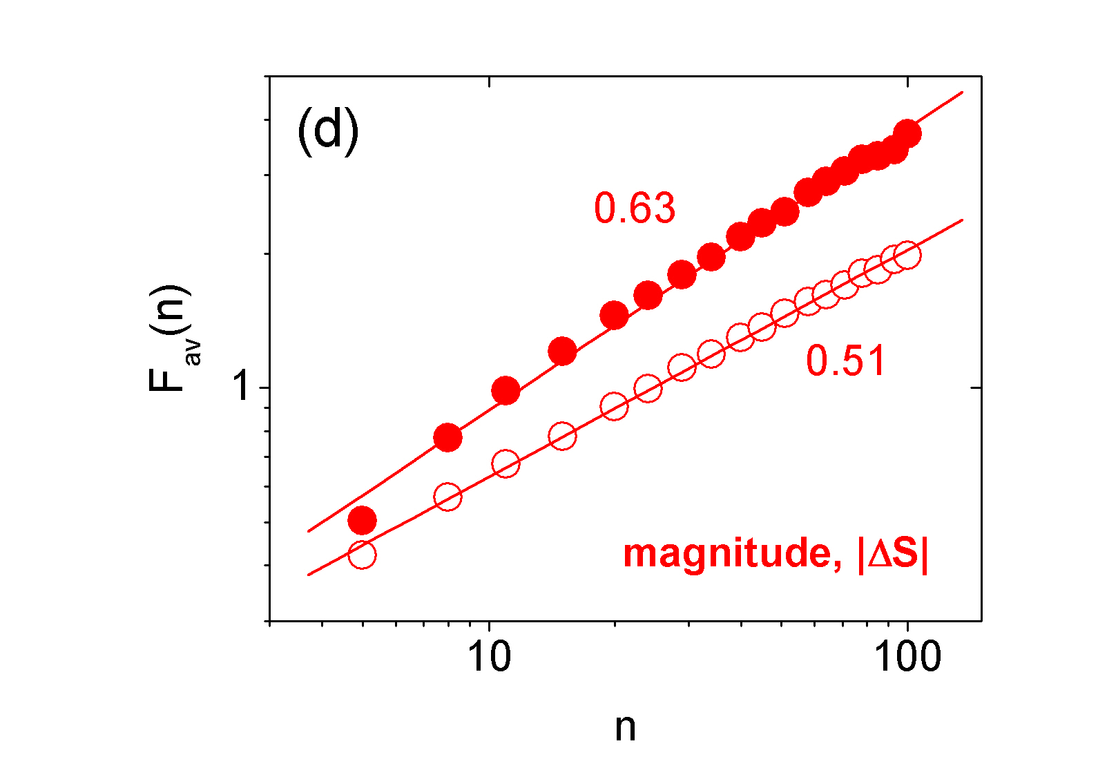
Figure 3: Analysis of temporal correlations in the data. $F_{av}(n)$ is an average of the DFA fluctuation function $F(n)$ calculated for several subseries. $F_{av}^{int}(n)$ is the average DFA fluctuation function obtained from integrated subseries. We investigate $F$ in the range $5\leq n\leq 100$. We also show $F_{av}$ and $F_{av}^{int}$ obtained from shuffled series (open circles). In all cases, the exponent $h$ is obtained by least square linear fits to the data. As expected, $h\simeq 0.5$ for all shuffled series. (a) $F_{av}(n)$ calculated from normalized energy series for earthquakes, $E/\sigma(E)$. The slope gives $h=0.57$. (b) $F_{av}(n)$ calculated from normalized energy series for crumpled plastic sheets, $S/\sigma(S)$. The linear fits gives $h=0.55$. (c) $F_{av}(n)$ calculated from normalized magnitude series for earthquakes, $|\Delta E|/\sigma(|\Delta E|)$, giving $h=0.66$. (d) $F_{av}(n)$ calculated from normalized magnitude series for crumpled plastic sheets, $|\Delta S|/\sigma(|\Delta S|)$. In this case, $h=0.63$. (e) $F_{av}^{int}(n)$ calculated from integrated sign series for earthquakes, $\mbox{sign}(\Delta E)$. The slope is $1.30$, giving $h=0.30$. (f) $F_{av}^{int}(n)$ calculated from integrated sign series for crumpled plastic sheets, $\mbox{sign}(\Delta S)$. The slope is also $1.30$, giving $h=0.30$.

Next, we investigate fractal properties in the output signal of the systems. For a given time series $x(i)$, the autocorrelation function is defined as $C(\tau)=\langle x(i)x(i+\tau)\rangle-\langle x(i)^{2}\rangle$. In order to reduce fluctuations in $C(\tau)$ it is common to obtain the root mean square fluctuation function $F(\tau)$, such that $F(\tau)^{2}=\sum_{i=1}^{\tau}\sum_{j=1}^{\tau}C(j-1)$[38]. The net displacement after $\tau$ steps is $y(\tau)=\sum_{i=1}^{\tau}x(i)$ and the root mean square fluctuation is defined as $\widehat{F}(\tau)=\sqrt{\langle\Delta y(\tau)^{2}\rangle-\langle\Delta y(\tau)\rangle^{2}}$, where $\Delta y(\tau)=y(\tau_{0}+\tau)-y(\tau_{0})$. For fractal series, $\widehat{F}(\tau)$ follows a power law behavior, $\widehat{F}(\tau)\sim\tau^{h}$, where $h$ is the scaling exponent which quantifies the degree of correlations. When $h>0.5$ ($h<0.5$) the series is long-range correlated (anti-correlated). Uncorrelated series present $h=0.5$. Short-range correlations also may exhibit $h=0.5$.

For nonstationary records, it is common to apply detrended fluctuation analysis (DFA)[34, 35] to investigate correlations in the data. For fractal series, the DFA root mean square fluctuation, $F(n)$, also follows a power law behavior,

$$F(n)\sim n^{h},$$ (4)

where $n$ is a time scale. Here we apply DFA method in order to quantify temporal correlations in the data.

The typical size of a given time series in the experiment of crumpled plastic sheets is $\sim 1016$ (20 samples). In order to perform a parallel analysis, we partition the energy series for earthquakes in subseries of size $1016$ (428 samples). For each subseries we obtain the DFA root mean square fluctuation, $F(n)$, and perform an average of $F(n)$ over all subseries - obtaining $F_{av}(n)$. Because the size of a typical subseries, we investigate $F(n)$ in the range $5<n<100$. Figures 3a and 3b shows $F_{av}(n)$ for the energy series for earthquakes and crumpled plastic sheets - $E$ and $S$. We find $h\simeq 0.55$ for both records suggesting weak correlations in the data. As expected, we find $h\simeq 0.5$ for shuffled series.

Starting from the sequence of energy increments, we also obtain two sub-series: magnitude of energy increments - $|\Delta E|$ and $|\Delta S|$ - and sign of energy increments - $\mbox{sign}[\Delta E]$ and $\mbox{sign}[\Delta S]$. The function $\mbox{sign}[\Delta x]$ assumes the values $-1$, $0$ or $1$ if the increment $\Delta x$ is negative, null or positive, respectively. For details of the magnitude-sign decomposition approach, see refs. [36, 37]. Figures 3c and 3d shows $F_{av}(n)$ for the magnitude series of energy increments for earthquakes and plastic sheets. For both records $h\simeq 0.65$ indicating long range correlations in the data. Figures 3e and 3f shows $F_{av}^{int}(n)$ - the average DFA fluctuation function obtained from integrated series - for the sign series of energy increments for earthquakes and plastic sheets. This previous integration is necessary in DFA method when $h<0.5$. For both records we find $h\simeq 0.30$ indicating anti-correlations in the data. As expected, shuffled magnitude and sign series exhibits $h\simeq 0.5$ indicating uncorrelated behavior. Notice the quantitative agreement between the values of $h$ for both systems.

The analysis reported here indicates remarkable similarities between two distinct out-of-equilibrium physical systems, providing a quantitative support for the analogy between earthquakes and crumpled films. Specifically, we show that for both signals i) the distribution of energy follows a power law with exponent $\alpha\simeq 3$; ii) the distribution of energy increments exhibits a common non-Gaussian shape in the range $1\leq\tau\leq 100$, with power law tails with exponent $\beta\simeq 3$; iii) the distribution of return intervals follows an exponential behavior; iv) the DFA power law exponent is $h\simeq 0.55$ for energy series, $h\simeq 0.65$ for magnitude series of energy increments and $h\simeq 0.30$ for sign series of energy increments in the range $5\leq n\leq 100$. These findings are consistent with the hypothesis that earthquakes and crumpled plastic sheets may be driven by common underlying mechanisms.

The nature of both processes analyzed here also presents analogies. It has been pointed that the energy stored in a crumpled material is originated in the buckling process while the film is crumpled, and it is mainly concentrated in the formed ridges[39, 40]. The nonequilibrium behavior observed in the relaxation process can be understood as a consequence of the frustration in the crossed ridges, characterizing a stress[41]. Moreover, it is known that Earth s crust can also exhibit buckling under viscous stresses on its layers[40].

Some phenomenological models, as the epidemic-type aftershock sequence model (ETAS)[42, 43], the continuous-time random walk models (CTRW)[43] and the Olami-Feder-Christensen model (OFC)[8, 44, 45] try to incorporate the main properties of the complex spatiotemporal behavior of earthquakes. Since the experiments with crumpled plastic sheets are simple and reproducible, they may be used as an additional data source to compare with artificial data. We hope that this analogy could provide some insight on the mechanisms behind the complex spatial and temporal behavior of earthquakes.

- [1] \NameTurcotte D. L. \REVIEWProc. Natl. Acad. Sci. U. S. A.9219956697.
- [2] \NameKagan Y. Y. \REVIEWPure Appl. Geophys.1551999233.
- [3] \NameBak P., Christensen K., Danon L. Scanlon T. \REVIEWPhys. Rev. Lett.882002178501.
- [4] \NameMega M. S., Allegrini P., Grigolini P., Latora V., Palatella L., Rapisarda A. Vincigerra S. \REVIEWPhys. Rev. Lett.902003188501.
- [5] \NameAbe S. Suzuki N. \REVIEWEurophys. Lett.652004581.
- [6] \NameCorral A. \REVIEWPhys. Rev. Lett.952005028501.
- [7] \NameSaichev A. Sornette D. \REVIEWPhys. Rev. Lett.972006078501.
- [8] \NameCaruso F., Pluchino A., Latora V., Vinciguerra S. Rapisarda A. \REVIEWPhys. Rev. E752007055101(R).
- [9] \NameLennartz S., Livina V. N., Bunde A. Havlin S. \REVIEWEPL81200869001.
- [10] \NameBalankin A. S., Matamoros D. M., Ortiz J. P., Ortiz M. P., Leon E. P. Ochoa D. S. \REVIEWEPL85200939001.
- [11] \NameAbe S. Suzuki N. \REVIEWEPL87200948008.
- [12] \NameCheng B., Epstein R. I., Guyer R. A. Young A. C. \REVIEWNature3821995518.
- [13] \NameAbe S. Suzuki N. \REVIEWPhysica A3192003552.
- [14] \NameAbe S. Suzuki N. \REVIEWPhysica D1932004310.
- [15] \NameGabaix X., Gopikrishnan P., Plerou V. Stanley H. E. \REVIEWNature4232003267.
- [16] \NamePenna T. J. P. Oliveira P. M. C. \REVIEWPhys. Rev. E521995R2168.
- [17] \NameGhashghaie S., Breymann W., Peinke J., Talkner P. Dodge Y. \REVIEWNature3811996767.
- [18] \NamePlerou V., Amaral L. A. N., Gopikrishnan P., Meyer M. Stanley H. E. \REVIEWNature4001999433.
- [19] \NameFukuda K., Amaral L. A. N. Stanley H. E. \REVIEWEurophys. Lett.622003189.
- [20] \NamePicoli S., Mendes R. S., Malacarne L. C. Papa A. R. R. \REVIEWEPL80200750006.
- [21] \NamePicoli S. Mendes R. S. \REVIEWPhys. Rev. E772008036105.
- [22] \NameSethna J. P., Dahmen K. A., Myers C. R. \REVIEWNature4102001242.
- [23] \NameMarder M., Deegan R. D. Sharon E. \REVIEWPhysics Today60200733.
- [24] \NameHoule P. A. Sethna J. P. \REVIEWPhys. Rev. E541996278.
- [25] \NameDidonna B. \REVIEWNature Materials52006167.
- [26] \NameMiguel M. C., Vespignani A., Zapperi S., Weiss J. Grasso J. R. \REVIEWNature4102001667.
- [27] \NameRicheton T., Weiss J. Louchet F. \REVIEWNature Materials42005465.
- [28] \NameCote P. J. Meisel L. V. \REVIEWPhys. Rev. Lett.6719911334.
- [29] \NameUrbach J. S., Madison R. C. Markert J. T. \REVIEWPhys. Rev. Lett.751995276.
- [30] http://www.ncedc.org/ncedc/catalog-search.html.
- [31] \NameTsallis, C. \REVIEWJournal of Statistical Physics521988479.
- [32] \NameTsallis C., Mendes R. S. Plastino A. R. \REVIEWPhysica A 2611998534.
- [33] \NamePicoli S., Mendes R. S., Malacarne L. C. Santos R. P. B. \REVIEWBrazilian Journal of Physics392009468.
- [34] \NamePeng C.-K. et al. \REVIEWPhys. Rev. E4919941685.
- [35] \NameBuldyrev S. V. et al. \REVIEWPhys. Rev. E5119955084.
- [36] \NameAshkenazy Y. et al. \REVIEWPhys. Rev. Lett.8620011900.
- [37] \NameAshkenazy Y. et al. \REVIEWPhysica A323200319.
- [38] \NameMontroll E. W. Shlesinger M. F. \BookNonequilibrium Phenomena II. From stochastic to hydrodynamics \PublNorth-Holland, Amsterdam \Year1984.
- [39] \NameWood A. J. \REVIEWPhysica A313200283.
- [40] \NameWitten T. A. \REVIEWRev. Mod. Phys.792007643.
- [41] \NameKramer E. M. Lobkovsky A. E. \REVIEWPhys. Rev. E5319961465.
- [42] \NameOgata Y. \REVIEWJ. Am. Stat. Assoc.8319889.
- [43] \NameSaichev A. Sornette D. \REVIEWPhys. Rev. Lett.972006078501.
- [44] \NameHelmstetter A. Sornette D. \REVIEWPhys. Rev. E662002061104.
- [45] \NameOlami Z., Feder H. J. S. Christensen K. \REVIEWPhys. Rev. Lett.6819921244.