Computation of the shortest path between two curves on a parametric surface by geodesic-like method

Abstract

In this paper, we present the geodesic-like algorithm for the computation of the shortest path between two objects on NURBS surfaces and periodic surfaces. This method can improve the distance problem not only on surfaces but in $\mathbb{R}^{3}$. Moreover, the geodesic-like algorithm also provides an efficient approach to simulate the minimal geodesic between two holes on a NURBS surfaces.

1 Introduction

Computing the distance between two objects on a surface plays an important role in many fields such as CAD, CAGD, robotics and computer graphics etc. In the Euclidean 3-space $\mathbb{R}^{3}$, it has a simple mathematical presentation as following:

$$\min_{p\in c_{1},\;q\in c_{2}}\|p-q\|,$$ (1)

where $c_{1}$ and $c_{2}$ are two objects in $\mathbb{R}^{3}$.

Although this representation is simple, however, it is hard to improve in general. The simplest case is the distance between two points and it can be estimated exactly by the Pythagorean theorem. If only one object is a point, then this problem is equivalent to the orthogonal projection problem, which has many applications [18, 19]. Many investigators have investigated the orthogonal projection problem. Chen et al. [3, 4], MaYL et al. [15] and Selimovic et al. [25] presented some effective methods that improve the distance problem between a point and a NURBS curve. Hu et al. [9] developed a good method to improve the orthogonal projection onto curves and surfaces. For the case that none of these objects is a single point, Kim [12] presented a method to estimate the distance between a canal surface and a simple surface in 2003, while Chen et al. [5] improved this problem on two implicit algebraic surfaces in 2006.

Unlike one can find many methods to investigate the distance problem in $\mathbb{R}^{3}$, there are few methods to study that on a curved surface. Maekawa [16] presented a very good method for solving the shortest path and the orthogonal projection problems on free-form parametric surfaces. Generally, the distance problem on a regular surface is more complicated than that in $\mathbb{R}^{3}$, even though the distance is just between two points on the surface, which is equivalent to find the length of the shortest path between them. We can find more information in reference [17]. This classical problem has many applications, such as in object segmentation, multi-scale image analysis and CAD etc. [2, 13, 24]. There are also many methods to estimate the shortest path on triangular mesh [14, 26], polyhedral [10, 21] and regular surface [11, 23] etc. These methods can be extend to improve the distance between one point and one curve or between two curves on surface but they are not effective methods.

In 2009, Chen [6] presents a new method to find geodesics on surfaces by the system of geodesic-like equations

$$\nabla E(u_{i},v_{j})=0.$$ (2)

In this paper, the distance problem on NURBS surfaces and parametric surfaces will be improved by the geodesic-like method with B-spline basis. In fact, the geodesic-like method can also estimate the distance between two objects in $\mathbb{R}^{3}$ but its efficiency is less than other algorithms that we known.

This paper is structured as follows. Section 2 describes the definition of the distance problem on regular surfaces and the notion of geodesic-like curves. We shall present our geodesic-like algorithm to estimate the distance between two objects on surfaces, especially on periodic surfaces, in section 3. Section 4 presents some examples about the distance problem on NURBS surfaces by simulations. Finally, we illustrate a discussion about our method and conclude this paper in Section 5.

2 Preliminaries

Let us introduce the distance problem between two curves on a regular surface and the system of geodesic-like equations in this section. Suppose that $S$ is a regular surface and $(U,\mathbf{x})$ is a system of coordinates on $S$. A curve $\gamma(t)=(x_{1}(t),x_{2}(t))$ is a geodesic curve in $(U,\mathbf{x})$ on $S$ if it satisfies the system of geodesic equations [1]

$$\frac{d^{2}x_{k}}{dt^{2}}+\sum_{i,j}\Gamma_{ij}^{k}\frac{dx_{i}}{dt}\frac{dx_{j}}{dt}=0,\mbox{~{}~{}~{}~{}}k=1,2.$$ (3)

From calculus of variation, a geodesic has an equivalent definition as below.

Definition 1

A geodesic on a regular surface is a critical point of the energy variations. That is, the geodesic $\gamma(t)$ is a critical point of the energy function

$$E(s)=\frac{1}{2}\int_{a}^{b}\|\frac{\partial f}{\partial t}(s,t)\|^{2}dt,$$ (4)

where $f(s,t)$ is any proper variation of $\gamma(t)$.

Here is a basic relationship between the length and energy functions.

Theorem 2

Let $S$ be a regular surface and $p,q\in S$ be two distinct points. If $\alpha$ is a shortest path between $p$ and $q$ on $S$, then $\alpha$ is a geodesic on $S$ which pass through $p$ and $q$. That is, the geodesic $\gamma(t)$ is a critical point of the length function

$$L(s)=\int_{a}^{b}\|\frac{\partial f}{\partial t}(s,t)\|dt.$$ (5)

The distance between two points on a surface $S$ is defined by the length of minimum path on $S$ from $p$ to $q$. Then

$$d(p,q)=\min_{\gamma\in\Gamma}L(\gamma),$$ (6)

where $\Gamma$ is the set of all paths on $S$ from $p$ to $q$ and $L(\gamma)$ is the length of the curve $\gamma$ on $S$. From Theorem 2, the set $\Gamma$ can be only considered the set of all geodesic on $S$ from $p$ to $q$.

Consider the parametric surface $S$ with a parametrization $\mathbf{x}:U\rightarrow\mathbb{R}^{3}$ and two curves $\mathbf{c}_{1}$ and $\mathbf{c}_{2}$ on $S$. For simplicity, we denote $c_{1},c_{2}:[a,b]\rightarrow U$ such that $\mathbf{c}_{1}=\mathbf{x}(c_{1}([a,b]))$ and $\mathbf{c}_{2}=\mathbf{x}(c_{2}[a,b]))$. Thus the distance between $\mathbf{c}_{1}$ and $\mathbf{c}_{2}$ on $S$ can be computed by

$$d(\mathbf{c}_{1},\mathbf{c}_{2})=\min_{s,t\in[a,b]}d(\mathbf{x}(c_{1}(s)),\mathbf{x}(c_{2}(t))).$$ (7)

That is, $d(\mathbf{c}_{1},\mathbf{c}_{2})$ is the length of minimal geodesic from $\mathbf{c}_{1}$ to $\mathbf{c}_{2}$. Equation (7) introduces a simple algorithm to improve this distance problem but it is too expansive. Let us describe it roughly.

Algorithm 1

First, we digitize the curves $\mathbf{c}_{1}$ and $\mathbf{c}_{2}$ to two sequences of points, $\{p_{i}\}_{i=0}^{m}$ and $\{q_{j}\}_{j=0}^{n}$, respectively. For each $i,j$, estimating the minimal geodesic $\gamma_{ij}$ between $p_{i}$ and $q_{j}$. Then the shortest path in $\{\gamma_{ij}\}_{(i,j)=(0,0)}^{(m,n)}$ approaches the minimal geodesic between $\mathbf{c}_{1}$ and $\mathbf{c}_{2}$ on surface $S$ when $m,n$ are large enough. Of course its length approaches the minimum distance between $\mathbf{c}_{1}$ and $\mathbf{c}_{2}$ on $S$.

Solve the geodesic between two fixed points is crucial to solve Algorithm 1. One can find many effective methods in the references [8, 11, 14, 21, 23, 26]. However, if the numbers of $\{p_{i}\}$ and $\{q_{j}\}$ are large, this algorithm becomes very slow. In fact, Algorithm 1 is the simplest and the slowest method to improve this problem.

We will improve the geodesic problem by the notion of geodesic-like curves [6].

Definition 3

Let $\mathbf{x}(u,v)$ be a parametrization of a regular surface $S$, $\mathbf{x}:U\subset\mathbb{R}^{2}\rightarrow S$. A curve $\tilde{\alpha}(s)$ on $U$ is called a geodesic-like curve of order $n+1$ on $S$ if $\tilde{\alpha}(s)=\sum_{i=0}^{n}N^{n}_{i}(s)(\tilde{u}_{i},\tilde{v}_{i})$ is a B-spline curve and satisfies the system of geodesic equations

$$(\nabla E)(\tilde{u}_{i},\tilde{v}_{j})=0,$$ (8)

where

$$E(u_{i},v_{j})=\frac{1}{2}\int_{a}^{b}\|\mathbf{x}(\alpha(t))\|^{2}dt$$

is the energy function of curve

$$\alpha(t)=\sum_{i=0}^{n}N_{i}^{n}(t)(u_{i},v_{i})$$

and $(\nabla E)(u_{i},v_{j})$ is the gradient of $E(u_{i},v_{j})$.

Equation (8) is called the system of standard geodesic-like equations. Although the system of geodesic-like equations are integral equations, they can be improved by the Newton’s method, the iterator method or other numerical methods [7, 11, 20, 22, 27] effectively.

Since any piecewise differential curve can be approximated by the B-spline curves, a geodesic-like curve approaches a geodesic on $S$ when the order of the geodesic-like curve is large enough. In the other words, we can estimate the distance between two points on $S$ via the minimal geodesic-like curves. We summarize this property as follows.

Theorem 4

Let $S$ be a parametric surface and let $\gamma:[0,1]\to S$ be a geodesic. Assume that the curve $\alpha_{n}=\sum_{i=0}^{n}N^{n}_{i}(t)(u_{i},v_{i})$ is the geodesic-like curve between $\gamma(0)$ and $\gamma(1)$ for each positive integer $n\geq 2$. Then

$$\lim_{n\rightarrow\infty}\alpha_{n}=\gamma.$$ (9)

3 Distance problem by geodesic-like algorithm

The system of geodesic-like equations provides an elegant method to improve the distance problem between two objects on surfaces. We are now in a position to introduce this method in this section. The parametrization $\mathbf{x}$ on $S$ is defined on $U=[a,b]\times[c,d]$. That is

$$\mathbf{x}:[a,b]\times[c,d]\rightarrow S\subset\mathbb{R}^{3}.$$

Let $c_{1}$ and $c_{2}$ be two differentiable parameterized curves on $S$ and

$$\begin{array}[]{l}c_{1}(s):[0,1]\rightarrow[a,b]\times[c,d]\cr c_{2}(t):[0,1]\rightarrow[a,b]\times[c,d].\end{array}$$

Thus $\mathbf{c}_{1}=\mathbf{x}(c_{1}([0,1]))$ and $\mathbf{c}_{2}=\mathbf{x}(c_{2}([0,1]))$ are two curves on $S$. To exclude the zero distance case from our consideration, we can assume that the two curves have no intersection. Denote $c_{1}(s)=(u_{0}(s),v_{0}(s))$ and $c_{2}(t)=(u_{n}(t),v_{n}(t))$ where $u_{0}$, $u_{n}:[0,1]\rightarrow[a,b]$ and $v_{0}$, $v_{n}:[0,1]\rightarrow[c,d]$ are all differentiable functions. Note that a B-spline curve $\alpha$ from $[0,1]$ into $[a,b]\times[c,d]$ with $\alpha(0)\in c_{1}$ and $\alpha(1)\in c_{2}$ always has the form as

$$\begin{array}[]{ll}\alpha(x)&=\sum_{i=1}^{n-1}N^{n}_{i}(x)(u_{i},v_{i})+N^{n}_{0}(x)c_{1}(s)+N^{n}_{n}(x)c_{2}(t)\cr&=\sum_{i=1}^{n-1}N^{n}_{i}(x)(u_{i},v_{i})+N^{n}_{0}(x)(u_{0}(s),v_{0}(s))+N^{n}_{n}(x)(u_{n}(t),v_{n}(t))\end{array}$$ (10)

where $x\in[0,1]$.

Hence, we rewrite the system of geodesic-like equations to the following three different forms. These formulas improve the distance between two curves on $S$, the orthogonal projection problem on $S$ and the shortest path between two points on $S$, respectively.

The system of geodesic-like equations between two curves:

From the equation (10), the parameters of the energy function $E$ are $s,t,u_{1},\cdots,u_{n-1},v_{1},\cdots,v_{n-1}$. The system of geodesic-like equations between two curves can be rewritten as

$$(\nabla E)=(E_{s},E_{t},E_{u_{1}},E_{u_{2}},\cdots,E_{u_{n}-1},E_{v_{1}},E_{v_{2}},\cdots,E_{v_{n}-1})=0$$ (11)

The system of geodesic-like equations between one point and one curve:

If $\mathbf{c}_{1}$ is a constat curve on $S$, then the derivative of $E$ about $t$ is vanish. Thus we obtain the geodesic-like equation between one point and one curve.

$$(\nabla E)=(E_{t},E_{u_{1}},E_{u_{2}},\cdots,E_{u_{n}-1},E_{v_{1}},E_{v_{2}},\cdots,E_{v_{n}-1})=0.$$ (12)

Of course, The orthogonal projection projection problem on surface cab be improve by equation (12).

The system of geodesic-like equations between two points:

Moreover, if $\mathbf{c}_{1}$ and $\mathbf{c}_{2}$ are both constant curves on $S$, then the geodesic-like equations between these two points is

$$(\nabla E)=(E_{u_{1}},E_{u_{2}},\cdots,E_{u_{n}-1},E_{v_{1}},E_{v_{2}},\cdots,E_{v_{n}-1})=0.$$ (13)

A curve satisfies one of equations (11) - (13) is called a geodesic-like curve between $\mathbf{c}_{1}$ and $\mathbf{c}_{2}$. Let us describe how to find the local minimal geodesic-like curve between two curves $\mathbf{c}_{1}$ and $\mathbf{c}_{2}$ on the surface $S$. In this algorithm, we solve the system of geodesic-like curve equations by the Newton’s method and the iterator method.

Algorithm 2

(Geodesic-like algorithm)

Step 1:

Given two closed curves $\mathbf{c}_{1}$ and $\mathbf{c}_{2}$ on the surface. Input an initial curve $\mathbf{\alpha}$ such that the endpoints of $\mathbf{\alpha}$ are on $\mathbf{c}_{1}$ and $\mathbf{c}_{2}$.

Step 2:

Solving the geodesic-like equations (equation (11) or (13)) by the initial curve $\mathbf{\alpha}$ and obtain a geodesic-like curve, which we still denote it by $\mathbf{\alpha}$, between $c_{1}$ and $c_{2}$.

Step 3:

If the set $(\mathbf{\alpha}\cap\mathbf{c}_{1})\cup(\mathbf{\alpha}\cap\mathbf{c}_{2})$ consists of the endpoints of $\mathbf{\alpha}$, then $\mathbf{\alpha}$ is the local minimal geodesic-like curve between $\mathbf{c}_{1}$ and $\mathbf{c}_{2}$. Otherwise, trimming away some parts of the curve $\mathbf{\alpha}$ such that the intersections of this trimmed curve, which we still denote it by $\mathbf{\alpha}$, and $(\bf{\alpha}\cap\mathbf{c}_{1})\cup(\mathbf{\alpha}\cap\mathbf{c}_{2})$ are only the endpoints of this trimmed curve (see Figure 1). Then repeat Step 2.

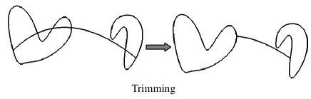
Figure 1: the method of trimmed curves

By Theorem 4, one will proceed by the geodesic-like algorithm to obtain the shortest path between $\mathbf{c}_{1}$ and $\mathbf{c}_{2}$ when the order $n$ is large enough. We summarize it as follows.

Theorem 5

Let $S$ be a parametric surface and $\mathbf{c}_{1}$, $\mathbf{c}_{2}$ be two closed curves on $S$. For each $n\geq 2$, $\tilde{\alpha}_{n}$ is the local minimal geodesic-like curve that obtained by the geodesic-like Algorithm (algorithm 2). If the set $\{\tilde{\alpha}_{n}\}$ is a convergent sequence, then there exists a local minimal geodesic $\gamma$ between $\mathbf{c}_{1}$ and $\mathbf{c}_{2}$ such that

$$\lim_{n\rightarrow\infty}\tilde{\alpha}_{n}=\gamma.$$ (14)

Moreover, $\tilde{\alpha}_{n}$ is orthogonal to $\mathbf{c}_{1}$ and $\mathbf{c}_{2}$ when $n$ is large enough.

3.1 Periodic surfaces

If $S$ is a periodic surface about one or two directions, then we may not obtain the local minimal geodesic-like curve by the Algorithm 2. It is because that the minimality of geodesics may not be preserved by the map of parametrization. To avoid this problem, we shall rewrite the domain $U$ of parametrization of $S$. For simplicity, we assume that the original domain of parametrization is $U=[0,1]\times[0,1]$ and then the parametrization $\mathbf{x}:[0,1]\times[0,1]\rightarrow S.$

One-directional periodic surface

Assume that $S$ is a parametrization surface with u-directional period and $\mathbf{x}$ is the parametrization on $S$. Its domain of parametrization, the $uv$-plane, is as in Figure 2. Then $\mathbf{x}(0,v)=\mathbf{x}(1,v)$ for each $v\in[0,1]$. Hence there is a function $\tilde{\mathbf{x}}:\mathbb{R}\times[0,1]\rightarrow S$ such that $\tilde{\mathbf{x}}(\tilde{u},v)=\mathbf{x}(u,v)$ for some $u\in[0,1]$ provided $(\tilde{u}-u)$ is an integer. Using the map $\tilde{\mathbf{x}}$, we can find two curves $c_{1}^{0}$ and $c_{1}^{1}$ from $[0,1]$ to $\mathbb{R}\times[0,1]$ such that $\tilde{\mathbf{x}}(c_{1}^{0}([0,1]))=\tilde{\mathbf{x}}(c_{1}^{1}([0,1]))=\mathbf{c}_{1}$ on $S$. Moreover, we assume that $c_{1}^{0}=c_{1}\subset[0,1]\times[0,1]$ and $c_{1}^{1}\subset[1,2]\times[0,1]$. Using Algorithm 2, the geodesic-likes curves from $c_{1}^{0}$ to $c_{2}$and from $c_{1}^{1}$ to $c_{2}$ on $U$ can be found and we denote them by $\gamma_{0}$ and $\gamma_{1}$ respectively (see Figure 2). Then the one in $\{\mathbf{x}(\gamma_{0}),\mathbf{x}(\gamma_{1})\}$ with smaller length is the local minimal geodesic-like curve between $\mathbf{c}_{1}$ and $\mathbf{c}_{2}$ on $S$.

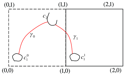
Figure 2: Local minimal geodesic-like curve on a one-directional periodic surface.

Two-directional periodic surface

If $S$ is a periodic surface about two directions, then we shall find $\tilde{\mathbf{x}}:\mathbb{R}\times\mathbb{R}\rightarrow S$ such that $\tilde{\mathbf{x}}(\tilde{u},\tilde{v})=\mathbf{x}(u,v)$ for some $u,v\in[0,1]$ if both $(\tilde{u}-u)$ and $(\tilde{v}-v)$ are integers. Similarly, we can find four curves $c_{1}^{0}\subset[0,1]\times[0,1]$, $c_{1}^{1}\subset[1,2]\times[0,1]$, $c_{1}^{2}\subset[0,1]\times[1,2]$ and $c_{1}^{3}\subset[1,2]\times[1,2]$ (see Figure 3) such that $\mathbf{x}(c_{1}^{i})=\mathbf{x}(c_{1})=\mathbf{c}_{1}$ on $S$ for $i=0,1,2,3$. Denote the minimal geodesic-like curve between $c_{1}^{i}$ and $c_{2}$ by $\gamma_{i}$ for $i=0,1,2,3$. Thus the minimal geodesic-like curve on $S$ between $\mathbf{c}_{1}$ and $\mathbf{c}_{2}$ on $S$ is the one in $\{\mathbf{x}(\gamma_{i})\}_{i=0}^{3}$ with the shortest length.

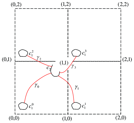
Figure 3: Local minimal geodesic-like curve on a two-directional periodic surface.

4 Simulations

To apply our method in practice, we present some examples by simulation. The geodesic-like curves in our simulations are all uniform quadratic B-spline curves in $\mathbb{R}^{2}$.

First we consider an open surface $S$ and two closed curves $\mathbf{c}_{1}$ and $\mathbf{c}_{2}$ on $S$ as in Figure 4. The surface $S$ is a cubic B-spline surface with (8,4) control points. The red curve in figure 4 is the local minimal geodesic-like curve of order 11 between $\mathbf{c}_{1}$ and $\mathbf{c}_{2}$ and its error is less than $10^{-6}$.

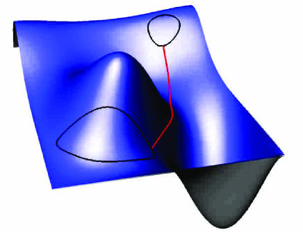
Figure 4: Distance between two closed curves on a NURBS surface

Secondly, a surface of revolution is an example of one-dimensional periodic surfaces. Figure 5 is the domain of parametrization ($uv$-plane) of the surface of revolution as in Figure 6. In Figure 5, there are two geodesic-like curves in the $uv$-plane, one is from $c_{1}^{0}$ to $c_{2}$ and the other is from $c_{1}^{1}$ to $c_{2}$. Then the image under parametrization of the shorter one is the local minimal geodesic-like curve between these two curves on the surface.

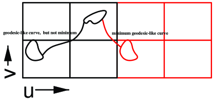
Figure 5: domain of parametrization of a $u$-periodic periodic surface

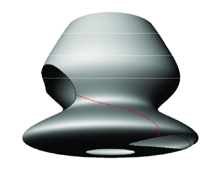
Figure 6: One-directional periodic surface

Thirdly, a typical example of two-dimensional periodic surfaces is the torus. Figure 7 is the domain of parametrization of a torus as in Figure 8. There are four geodesic-like curves in the $uv$-plane. Therefore, the image under parametrization of the shortest one is the local minimal geodesic-like curve between two closed curves on the torus.

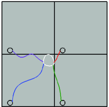
Figure 7: Distance between two closed curves on torus (uv-plane)

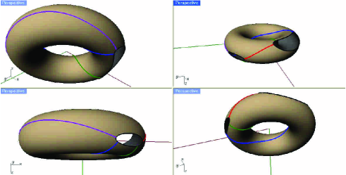
Figure 8: Distance between two closed curves on torus

Lastly, we construct a face model as in Figure 9 by NURBS surface and find the minimal geodesic-like curves between two holds (the eyes) on the surface. The data in Figure10 are about the geodesic-like curves of different orders between the two holes in Figure 9. Here in Figure 10 the order means the number of control points while error(%) is the percentage of error, which is defined by

$$\mbox{error(\%) }=\frac{\mbox{ Length }-\mbox{ minimum distance}}{\mbox{ minimum distance}}\times 100\%.$$ (15)

The red curve in Figure 9 is the local minimal geodesic-like curve of order 30 and the green curve is the exact minimal geodesic between two holes. Then the lengths of geodesic-like curves constructed by our method approaches the minimum distance between the two holes. To deserve to be mentioned, error(%) will be less than $10^{-7}$ provided the geodesic-like curve is constructed by 60 control points. It proposes that the geodesic-like algorithm has increased actually computational efficiency of this simulation .

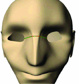
Figure 9: The distance between two holds on a face model

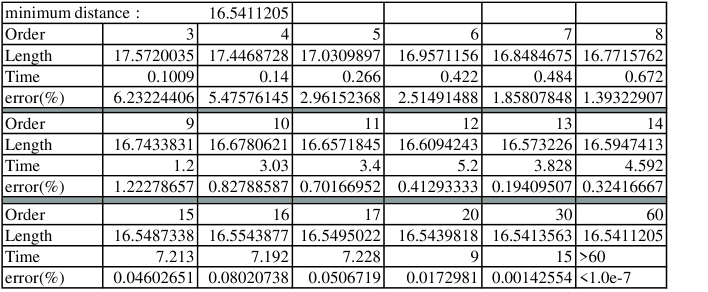
Figure 10: The table of the distance between two holds on a face model with different orders

5 Discussion

The geodesic-like algorithm provides an effective and reliable computation of shortest paths between two curves on surfaces. For computing the shortest paths between two curves on $\mathbb{R}^{3}$, our method is comparable with other well-known methods. Especially, the construction of geodesic-like curves only bases on the uniform quadratic B-spline curves since it is enough to us to consider the geodesic-like curves in the plane. Significatively, our method can be extended to solve the distance problem between any two objects on surfaces and the distance problem in higher dimension.

To solve the system of geodesic-like equations, however, Newton’s method is too expansive. Moreover, it can only solve local minimal geodesic-like curves but not global minimum ones. In the future investigation, we expect to find a numerical method to solve efficiently all local minimal geodesic-like curves between two objects on surfaces to overcome these problems.

References

- [1] M.p. Do Carmo, Differential Geometry of Curves and Surfaces. Prentice-Hall, Englewood Cliffs, NJ(1976).
- [2] V. Caselles, R. Kimmel, G. Sapiro, Geodesic active contours, Int. J. Comput. Vision 22 (1) (1997) 61 V71.
- [3] XD Chen, H Su, b JH Yong, JC Paul , JG Sun, A counterexample on point inversion and projection for NURBS curve. CAGD 24 (2007) 302.
- [4] X.-D. Chen, J.-H. Yong, Guozhao Wang, J.-C. Paul, Gang Xu, Computing the minimum distance between a point and a NURBS curve. CAD 40 (2008)1051-1054.
- [5] X.-D. Chen, J.-H. Yonga, G.-Q. Zhenga, J.-C. Paula, J.-G. Suna, Computing minimum distance between two implicit algebraic surfaces CAD 38 (2006) 1053-1061.
- [6] S.-G. Chen. Geodesic-like curves on parametric surfaces. submitted to CAGD (2009).
- [7] JM Gutierrez, MA Hernandez . An acceleration of Newton’s method: Super- Halley method. Applied Mathematics and Computation 117 (2001) 223-239.
- [8] I. Hotz, H. Hagen, Visualizing geodesics. In: Proceedings IEEE Visualization, Salt Lake City, UT (2000) 311-318.
- [9] SM Hu, J. Wallner, A second order algorithm for orthogonal projection onto curves and surfaces. CAGD 22 (2005) 251-60.
- [10] T. Kanai, H. Suzuki, Approxmiate shortest path on a polyhedral surface and its applications. CAD 33 (2001) 801-811
- [11] Emin Kasap, Mustafa Yapici, F. Talay Akyildiz, A numerical study for computation of geodesic curves Applied Mathematics and Computation 171 (2005) 1206-1213.
- [12] K.-J. Kim, Minimum distance between a canal surface and a simple surface. CAD 35 (2003) 871-879.
- [13] R. Kimmel, Intrinsic scale space for images on surfaces: the geodesic curvature flow, Graph. Models Image Process 59 (1997) 365 V372.
- [14] Dimas Martinez, Luiz Velho. Paulo C. Carvalho, Computing geodesics on triangular meshes. Computer & Graphics. volume 29 (2005) 667-675.
- [15] YL Ma, WT Hewitt, Point inversion and projection for NURBS curve and surface: Control polygon approach. CAGD 20 (2003) 79-99.
- [16] T. Maekawa, Computation of shortest path on free-form parametric surfaces, Journal of Mechanical Design, Transactions of ASME 118 (1996) 499-508.
- [17] N. Patrikalakis, T. Maekawa, Shape interrogation for computer aided design and manufacturing. Springer (2001).
- [18] L. Piegl, W. Tiller, Parametrization for surface fitting in reverse engineering. CAD 33 (2001) 593-603.
- [19] J. Pegna, FE. Wolter, Surface curve design by orthogonal projection of space curves onto free-form surfaces. Journal of Mechanical Design, ASME Transactions 18 (1996) 45-52.
- [20] E. Polak, Optimization, algorithms and consistent approximations, Berlin (Heidelberg, NY): Springer-Verlag (1997).
- [21] K. Polthier, M. Schmies, In: Hege, H.C., Polthier, H.K. (Eds.), Straightest Geodesics On Polyhedral Surfaces in Mathematical Visualization. Springer-Verlag, Berlin (1998).
- [22] WH Press, SA Teukolsky, WT Vetterling, BP Flannery, Numerical recipes in C: The art of scientific computing. 2nd ed.NewYork: Cambridge University Press (1992).
- [23] G. V. V. Ravi Kumar, Prabha Srinivasan, V. Devaraja Holla, K. G. Shastry, B. G. Prakash, Geodesic curve computations on surfaces, CAGD 20 (2003) 119-133
- [24] J. Sánchez-Reyesa, R. Doradob, Constrained design of polynomial surfaces from geodesic curves. CAD 40 (2008) 49-55.
- [25] I. Selimovic, Improved algorithms for the projection of points on NURBS curves and surfaces. CAGD 23 (2006) 439-445.
- [26] V. Surazhsky, T. Surazhsky, D. Kirsanov, S. Gortler, H. Hoppe. Fast exact and approximate geodesics on meshes. ACM Transactions on Graphics (Proc. of SIGGRAPH 2005), 24(3), 553-560.
- [27] Ye Y. Combining binary search and Newton’s method to compute real roots for a class of real functions. Journal of Complexity 1994;10(3):271-280.