Spinon Phonon Interaction and Ultrasonic Attenuation in Quantum Spin Liquids
Yi Zhou
Department of Physics and Zhejiang Institute of Modern Physics, Zhejiang University, Hangzhou, 310027, P.R. China
Patrick A Lee
Department of Physics, Massachusetts Institute of Technology,
77 Massachusetts Avenue, Cambridge, MA 02139
Abstract
Several experimental candidates for quantum spin liquids have been discovered in the past few years which appear to support gapless fermionic S = 1 2 𝑆 1 2 S={1\over 2} U ( 1 ) 𝑈 1 U(1) T c subscript 𝑇 𝑐 T_{c} U ( 1 ) 𝑈 1 U(1)
pacs: 71.27.+a,75.10.Jm,71.10.-w,74.70.Kn
Quantum spin liquid in dimensions greater than one is a long sought state of matter which has eluded experimental
investigation until recently.Lee08 1 2 1 2 {1\over 2} U ( 1 ) 𝑈 1 U(1) Z 2 subscript 𝑍 2 Z_{2} κ − limit-from 𝜅 \kappa- 2 Cu2 (CN)3 salt (abbreviated as ET) Kanoda03 Itou08 2 (EtMe3 Sb) which we shall refer to as dmit.
Both materials are Mott insulators on an approximate triangular lattice with spin 1 2 1 2 \frac{1}{2} J ≈ 250 𝐽 250 J\approx 250 SYamashita κ 𝜅 \kappa κ / T 𝜅 𝑇 \kappa/T MYamashita09 κ / T 𝜅 𝑇 \kappa/T MYamashita10
Initial theoretical work pointed to a state where spinons form a Fermi surface and are coupled to U ( 1 ) 𝑈 1 U(1) Motrunich ; SSLee Manna 1 / T 1 T 1 subscript 𝑇 1 𝑇 1/T_{1}T Itou10 Grover
Two other examples, the Kagome compound ZnCu3 (OH)6 Cl2 and the three dimensional hyper-Kagome Na4 Ir3 O8
also satisfy the condition of being spin liquids in that they do not show magnetic order and both are characterized
by gapless excitations.Kagome07 ; Takagi07
In this paper we address two questions. First, how do the spinons couple to phonons, and, secondly, is there a way
to unambiguously identify the pairing transition of spinons? As we shall see, the two questions are related because
the attenuation of transverse sound turns out to be sensitive to the gauge magnetic field fluctuations and is
a sensitive probe of the Meissner effect of gauge magnetic field at the onset of any pairing instability.
The coupling of electrons to phonons is often discussed in terms of the screened Coulomb coupling between electrons
and nuclei and one may have the impression that the charge neutral spinon may couple differently. It turns out that
in the long wavelength limit, the coupling matrix elements are exactly the same. This is because in this limit
the coupling can be viewed as a distortion of the Fermi surface by the local stress of the unit cell and is the same
whether the fermions are charged or not. Recently the spin phonon coupling was discused
in terms of interactions mediated by gauge fields
with the conclusion that the coupling is
comparable to the electron phonon coupling.Mross
We begin with a derivation of the spinon phonon coupling following Blount’s discussion of the electron phonon problem
which was also used in Tsuneto’s theory of ultrasound attenuation.Blount ; Tsuneto E 0 ( 𝒌 ) subscript 𝐸 0 𝒌 E_{0}(\bm{k}) E 0 ( 𝒌 ) subscript 𝐸 0 𝒌 E_{0}(\bm{k})
H 0 = E 0 ( 𝒑 ) + V imp ( 𝒓 ′ ) , subscript 𝐻 0 subscript 𝐸 0 𝒑 subscript 𝑉 imp superscript 𝒓 ′ H_{0}=E_{0}(\bm{p})+V_{\rm imp}({\bm{r}}^{\prime}), (1)
where 𝒑 = − i ∂ ∂ 𝒓 𝒑 𝑖 𝒓 {\bm{p}}=-i{\partial\over\partial{\bm{r}}} V imp subscript 𝑉 imp V_{\rm imp} 𝒓 ′ superscript 𝒓 ′ {\bm{r}}^{\prime} δ 𝑹 ( 𝒓 ′ , t ) 𝛿 𝑹 superscript 𝒓 ′ 𝑡 \delta{\bm{R}}({\bm{r}}^{\prime},t) 𝒓 ′ superscript 𝒓 ′ {\bm{r}}^{\prime} 𝒓 = 𝒓 ′ − δ 𝑹 ( 𝒓 ′ , t ) 𝒓 superscript 𝒓 ′ 𝛿 𝑹 superscript 𝒓 ′ 𝑡 {\bm{r}}={\bm{r}}^{\prime}-\delta{\bm{R}}({\bm{r}^{\prime}},t) U = e i S 𝑈 superscript 𝑒 𝑖 𝑆 U=e^{iS} S = 1 2 ( 𝒑 ⋅ δ 𝑹 + δ 𝑹 ⋅ 𝒑 ) . 𝑆 1 2 ⋅ 𝒑 𝛿 𝑹 ⋅ 𝛿 𝑹 𝒑 S={1\over 2}({\bm{p}}\cdot\delta{\bm{R}}+\delta{\bm{R}}\cdot{\bm{p}}).
H 0 + H 1 = U H U − 1 + i ∂ U ∂ t U − 1 subscript 𝐻 0 subscript 𝐻 1 𝑈 𝐻 superscript 𝑈 1 𝑖 𝑈 𝑡 superscript 𝑈 1 H_{0}+H_{1}=UHU^{-1}+i{\partial U\over\partial t}U^{-1} (2)
where H 0 subscript 𝐻 0 H_{0} 𝒓 ′ superscript 𝒓 ′ {\bm{r}}^{\prime} 𝒓 𝒓 {\bm{r}} δ 𝑹 𝛿 𝑹 \delta{\bm{R}}
H 1 = i [ S , E 0 ( 𝒑 ) ] + i 2 ∑ α { ∇ α , ∂ S ∂ t δ R α } subscript 𝐻 1 𝑖 𝑆 subscript 𝐸 0 𝒑 𝑖 2 subscript 𝛼 subscript ∇ 𝛼 𝑆 𝑡 𝛿 subscript 𝑅 𝛼 H_{1}=i[S,E_{0}(\bm{p})]+{i\over 2}\sum_{\alpha}\left\{\nabla_{\alpha},{\partial S\over\partial t}\delta R_{\alpha}\right\} (3)
Next we write δ 𝑹 ∼ e i ( 𝒒 ⋅ 𝒓 − ω t ) similar-to 𝛿 𝑹 superscript 𝑒 𝑖 ⋅ 𝒒 𝒓 𝜔 𝑡 \delta\bm{R}\sim e^{i({\bm{q}}\cdot{\bm{r}}-\omega t)} ω = v s q 𝜔 subscript 𝑣 𝑠 𝑞 \omega=v_{s}q v s subscript 𝑣 𝑠 v_{s} 3 ∇ δ 𝑹 bold-∇ 𝛿 𝑹 {\bm{\nabla}}\delta{\bm{R}} ∂ δ 𝑹 ∂ t 𝛿 𝑹 𝑡 {\partial\delta{\bm{R}}\over\partial t}
H 1 = ∑ α β ∂ δ R β ∂ r α p β v α + i 𝒑 ⋅ ∂ δ 𝑹 ∂ t subscript 𝐻 1 subscript 𝛼 𝛽 𝛿 subscript 𝑅 𝛽 subscript 𝑟 𝛼 subscript 𝑝 𝛽 subscript 𝑣 𝛼 ⋅ 𝑖 𝒑 𝛿 𝑹 𝑡 H_{1}=\sum_{\alpha\beta}{\partial\delta R_{\beta}\over\partial r_{\alpha}}p_{\beta}v_{\alpha}+i{\bm{p}}\cdot{\partial\delta{\bm{R}}\over\partial t} (4)
where v α ( 𝒑 ) = d E 0 / d 𝒑 α subscript 𝑣 𝛼 𝒑 𝑑 subscript 𝐸 0 𝑑 subscript 𝒑 𝛼 v_{\alpha}(\bm{p})=dE_{0}/d{\bm{p}}_{\alpha} 4 E ( 𝒑 ) 𝐸 𝒑 E(\bm{p}) 𝒑 𝒑 \bm{p} 4 ω k F 𝜔 subscript 𝑘 𝐹 \omega k_{F} ω k F / ( q k F v F ) = v s / v F 𝜔 subscript 𝑘 𝐹 𝑞 subscript 𝑘 𝐹 subscript 𝑣 𝐹 subscript 𝑣 𝑠 subscript 𝑣 𝐹 \omega k_{F}/(qk_{F}v_{F})=v_{s}/v_{F}
Now we introduce the phonons
H ph = ∑ 𝒒 , λ , σ ω 𝒒 λ a 𝒒 λ † a 𝒒 λ subscript 𝐻 ph subscript 𝒒 𝜆 𝜎
subscript 𝜔 𝒒 𝜆 subscript superscript 𝑎 † 𝒒 𝜆 subscript 𝑎 𝒒 𝜆 H_{\rm ph}=\sum_{{\bm{q}},\lambda,\sigma}\omega_{{\bm{q}}\lambda}a^{\dagger}_{{\bm{q}}\lambda}a_{{\bm{q}}\lambda} (5)
where λ 𝜆 \lambda ε ^ 𝒒 λ subscript ^ 𝜀 𝒒 𝜆 \hat{\varepsilon}_{{\bm{q}}\lambda} δ 𝑹 𝛿 𝑹 \delta{\bm{R}} 4
H s − ph = ∑ 𝒌 , 𝒒 , λ , σ M 𝒌 λ ( 𝒒 ) f 𝒌 + 𝒒 σ † f 𝒌 σ ( a 𝒒 λ + a − 𝒒 λ † ) , subscript 𝐻 s ph subscript 𝒌 𝒒 𝜆 𝜎
subscript 𝑀 𝒌 𝜆 𝒒 subscript superscript 𝑓 † 𝒌 𝒒 𝜎 subscript 𝑓 𝒌 𝜎 subscript 𝑎 𝒒 𝜆 subscript superscript 𝑎 † 𝒒 𝜆 H_{\rm s-ph}=\sum_{{\bm{k}},{\bm{q}},\lambda,\sigma}M_{{\bm{k}}\lambda}({\bm{q}})f^{\dagger}_{{\bm{k}}+{\bm{q}}\sigma}f_{{\bm{k}}\sigma}(a_{{\bm{q}}\lambda}+a^{\dagger}_{-{\bm{q}}\lambda}), (6)
M 𝒌 λ ( 𝒒 ) = ( 𝒌 ⋅ ε ^ 𝒒 λ ) [ 𝒒 ⋅ 𝒗 ( 𝒌 ) ] ( 2 ρ ion ω 𝒒 λ ) − 1 / 2 subscript 𝑀 𝒌 𝜆 𝒒 ⋅ 𝒌 subscript ^ 𝜀 𝒒 𝜆 delimited-[] ⋅ 𝒒 𝒗 𝒌 superscript 2 subscript 𝜌 ion subscript 𝜔 𝒒 𝜆 1 2 M_{{\bm{k}}\lambda}(\bm{q})=({\bm{k}}\cdot{\hat{\varepsilon}}_{{\bm{q}}\lambda})[{\bm{q}}\cdot{\bm{v}}({\bm{k}})](2\rho_{\rm ion}\omega_{{\bm{q}}\lambda})^{-1/2} (7)
where ρ ion subscript 𝜌 ion \rho_{\rm ion} 𝒂 𝒂 {\bm{a}} E ( 𝒌 ) = k 2 / 2 m 𝐸 𝒌 superscript 𝑘 2 2 𝑚 E(\bm{k})=k^{2}/2m
H 0 s = ∑ 𝒌 , σ 1 2 m ( 𝒌 + 𝒂 ) 2 f 𝒌 σ † f 𝒌 σ . subscript 𝐻 0 𝑠 subscript 𝒌 𝜎
1 2 𝑚 superscript 𝒌 𝒂 2 subscript superscript 𝑓 † 𝒌 𝜎 subscript 𝑓 𝒌 𝜎 H_{0s}=\sum_{\bm{k},\sigma}{1\over 2m}({\bm{k}}+{\bm{a}})^{2}f^{\dagger}_{{\bm{k}}\sigma}f_{{\bm{k}}\sigma}. (8)
In addition we have the impurity scattering term
H imp = ∑ i σ v imp ( 𝒓 i ) f σ † ( 𝒓 i ) f σ ( 𝒓 i ) subscript 𝐻 imp subscript 𝑖 𝜎 subscript 𝑣 imp subscript 𝒓 𝑖 subscript superscript 𝑓 † 𝜎 subscript 𝒓 𝑖 subscript 𝑓 𝜎 subscript 𝒓 𝑖 H_{\rm imp}=\sum_{i\sigma}v_{\rm imp}({\bm{r}}_{i})f^{\dagger}_{\sigma}({\bm{r}}_{i})f_{\sigma}({\bm{r}}_{i}) τ 𝜏 \tau l = v F τ 𝑙 subscript 𝑣 𝐹 𝜏 l=v_{F}\tau
From this point on we can discuss the sound attenuation in spin liquids in parallel with the theory for metals
and superconductors. Historically the first discussion was in the hydrodynamic regime valid for q l ≪ 1 much-less-than 𝑞 𝑙 1 ql\ll 1 Mason ; Morse τ s subscript 𝜏 𝑠 \tau_{s}
τ s L = 1 ρ ion v s 2 ( 4 3 η + χ ) , τ s T = 1 ρ ion v s 2 η formulae-sequence superscript subscript 𝜏 𝑠 𝐿 1 subscript 𝜌 ion superscript subscript 𝑣 𝑠 2 4 3 𝜂 𝜒 superscript subscript 𝜏 𝑠 𝑇 1 subscript 𝜌 ion superscript subscript 𝑣 𝑠 2 𝜂 \tau_{s}^{L}={1\over\rho_{\rm ion}v_{s}^{2}}\left({4\over 3}\eta+\chi\right),\tau_{s}^{T}={1\over\rho_{\rm ion}v_{s}^{2}}\eta (9)
for the longitudinal and transverse sound, respectively, where η , χ 𝜂 𝜒
\eta,\chi α 𝛼 \alpha l ph subscript 𝑙 ph l_{\rm ph} k = ( ω / v s ) ( 1 + i ω τ s ) − 1 / 2 𝑘 𝜔 subscript 𝑣 𝑠 superscript 1 𝑖 𝜔 subscript 𝜏 𝑠 1 2 k=(\omega/v_{s})(1+i\omega\tau_{s})^{-1/2} α = ω 2 τ s 2 v s 𝛼 superscript 𝜔 2 subscript 𝜏 𝑠 2 subscript 𝑣 𝑠 \alpha={\omega^{2}\tau_{s}\over 2v_{s}} ω τ s ≪ 1 much-less-than 𝜔 subscript 𝜏 𝑠 1 \omega\tau_{s}\ll 1 η = 1 15 N ( 0 ) m 2 v F 4 τ 𝜂 1 15 𝑁 0 superscript 𝑚 2 superscript subscript 𝑣 𝐹 4 𝜏 \eta={1\over 15}N(0)m^{2}v_{F}^{4}\tau N ( 0 ) 𝑁 0 N(0) χ 𝜒 \chi ≪ η much-less-than absent 𝜂 \ll\eta
The hydrodynamic theory was extended by Pippard to all values of q l 𝑞 𝑙 ql Pippard q l ≳ 1 greater-than-or-equivalent-to 𝑞 𝑙 1 ql\gtrsim 1
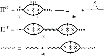
Figure 1: Feynman digrams for phonon self energy.
Let us first re-derive the results for metals. We compute the phonon self energy Π ( q , ω ) Π 𝑞 𝜔 \Pi(q,\omega) G ret ( adv ) ( k , ω ) = ( ω − ξ k ± i / 2 τ ) − 1 subscript 𝐺 ret adv 𝑘 𝜔 superscript plus-or-minus 𝜔 subscript 𝜉 𝑘 𝑖 2 𝜏 1 G_{\rm ret(adv)}(k,\omega)=(\omega-\xi_{k}\pm i/2\tau)^{-1} ξ k = k 2 / 2 m − μ subscript 𝜉 𝑘 superscript 𝑘 2 2 𝑚 𝜇 \xi_{k}=k^{2}/2m-\mu k TF − 1 superscript subscript 𝑘 TF 1 k_{\rm TF}^{-1} q − 1 superscript 𝑞 1 q^{-1} M ~ k λ subscript ~ 𝑀 𝑘 𝜆 \tilde{M}_{k\lambda} 7 M ~ 𝒌 λ ( 𝒒 ) = [ ( 𝒌 ⋅ ε ^ 𝒒 λ ) ( 𝒌 ⋅ 𝒒 ) − 1 3 k 2 ( 𝒒 ⋅ ε ^ 𝒒 λ ) ] / m 2 ρ ion ω 𝒒 λ subscript ~ 𝑀 𝒌 𝜆 𝒒 delimited-[] ⋅ 𝒌 subscript ^ 𝜀 𝒒 𝜆 ⋅ 𝒌 𝒒 1 3 superscript 𝑘 2 ⋅ 𝒒 subscript ^ 𝜀 𝒒 𝜆 𝑚 2 subscript 𝜌 ion subscript 𝜔 𝒒 𝜆 \tilde{M}_{{\bm{k}}\lambda}(\bm{q})=[({\bm{k}}\cdot\hat{\varepsilon}_{{\bm{q}}\lambda})({\bm{k}}\cdot{\bm{q}})-{1\over 3}k^{2}({\bm{q}}\cdot\hat{\varepsilon}_{{\bm{q}}\lambda})]/m\sqrt{2\rho_{\rm ion}\omega_{{\bm{q}}\lambda}} Blount 7 𝒌 𝒌 \bm{k} 𝒒 𝒒 \bm{q} Π ( 0 ) superscript Π 0 \Pi^{(0)} Π ( 1 ) superscript Π 1 \Pi^{(1)} 𝒋 𝒋 \bm{j} 𝒋 ⋅ 𝑨 ⋅ 𝒋 𝑨 {\bm{j}}\cdot{\bm{A}}
D ret EM = 1 i ω σ ⟂ ( q , ω ) + ω 2 − c 2 q 2 superscript subscript 𝐷 ret EM 1 𝑖 𝜔 subscript 𝜎 perpendicular-to 𝑞 𝜔 superscript 𝜔 2 superscript 𝑐 2 superscript 𝑞 2 D_{\rm ret}^{\rm EM}={1\over i\omega\sigma_{\perp}(q,\omega)+\omega^{2}-c^{2}q^{2}} (10)
and c 𝑐 c ω 2 superscript 𝜔 2 \omega^{2} 10 σ ⟂ ( q , ω ) = g σ 0 subscript 𝜎 perpendicular-to 𝑞 𝜔 𝑔 subscript 𝜎 0 \sigma_{\perp}(q,\omega)=g\sigma_{0} σ 0 = e 2 n τ / m subscript 𝜎 0 superscript 𝑒 2 𝑛 𝜏 𝑚 \sigma_{0}=e^{2}n\tau/m
g = 3 2 a Re [ s 2 ( a ) − s 0 ( a ) ] , s n ( a ) = 1 2 i ∫ − 1 1 𝑑 u u n u + i / a , formulae-sequence 𝑔 3 2 𝑎 Re delimited-[] subscript 𝑠 2 𝑎 subscript 𝑠 0 𝑎 subscript 𝑠 𝑛 𝑎 1 2 𝑖 subscript superscript 1 1 differential-d 𝑢 superscript 𝑢 𝑛 𝑢 𝑖 𝑎 g={3\over 2a}{\rm Re}[s_{2}(a)-s_{0}(a)],\,\,s_{n}(a)={1\over 2i}\int^{1}_{-1}du{u^{n}\over u+i/a},
where a = q l / ( 1 + i ω τ ) 𝑎 𝑞 𝑙 1 𝑖 𝜔 𝜏 a=ql/(1+i\omega\tau) ω τ ≪ 1 much-less-than 𝜔 𝜏 1 \omega\tau\ll 1 a = q l 𝑎 𝑞 𝑙 a=ql g → 1 − 2 15 ( q l ) 2 → 𝑔 1 2 15 superscript 𝑞 𝑙 2 g\rightarrow 1-{2\over 15}(ql)^{2} q l ≪ 1 much-less-than 𝑞 𝑙 1 ql\ll 1 g → 3 π 4 ( q l ) − 1 → 𝑔 3 𝜋 4 superscript 𝑞 𝑙 1 g\rightarrow{3\pi\over 4}(ql)^{-1} q l ≫ 1 much-greater-than 𝑞 𝑙 1 ql\gg 1 ( q l ≫ 1 ) much-greater-than 𝑞 𝑙 1 (ql\gg 1) 10 N ( 0 ) ω / v F q 𝑁 0 𝜔 subscript 𝑣 𝐹 𝑞 N(0)\omega/v_{F}q ( q l ≪ 1 ) much-less-than 𝑞 𝑙 1 (ql\ll 1) k 0 − 1 superscript subscript 𝑘 0 1 k_{0}^{-1} k 0 2 = ω σ 0 / c 2 superscript subscript 𝑘 0 2 𝜔 subscript 𝜎 0 superscript 𝑐 2 k_{0}^{2}=\omega\sigma_{0}/c^{2}
The diagrams are evaluated to give (see supplementary materials for details)
Im Π ret ( 0 ) = ω N ( 0 ) k F 3 4 ρ ion m v s 2 s 1 ( q l ) − s 3 ( q l ) i q l . Im subscript superscript Π 0 ret 𝜔 𝑁 0 superscript subscript 𝑘 𝐹 3 4 subscript 𝜌 ion 𝑚 superscript subscript 𝑣 𝑠 2 subscript 𝑠 1 𝑞 𝑙 subscript 𝑠 3 𝑞 𝑙 𝑖 𝑞 𝑙 {\rm Im}\Pi^{(0)}_{\rm ret}={\omega N(0)k_{F}^{3}\over 4\rho_{\rm ion}mv_{s}^{2}}{s_{1}(ql)-s_{3}(ql)\over iql}. (11)
On the other hand, Π ret ( 1 ) superscript subscript Π ret 1 \Pi_{\rm ret}^{(1)} k 0 subscript 𝑘 0 k_{0} q 𝑞 q l − 1 superscript 𝑙 1 l^{-1} c 2 q 2 ≪ ω σ ⟂ ( q , ω ) much-less-than superscript 𝑐 2 superscript 𝑞 2 𝜔 subscript 𝜎 perpendicular-to 𝑞 𝜔 c^{2}q^{2}\ll\omega\sigma_{\perp}(q,\omega) D ret EM = ( i ω σ ⟂ ( q , ω ) ) − 1 superscript subscript 𝐷 ret EM superscript 𝑖 𝜔 subscript 𝜎 perpendicular-to 𝑞 𝜔 1 D_{\rm ret}^{\rm EM}=\left(i\omega\sigma_{\perp}(q,\omega)\right)^{-1} q ≪ k 0 much-less-than 𝑞 subscript 𝑘 0 q\ll k_{0} q l ≪ 1 much-less-than 𝑞 𝑙 1 ql\ll 1 q 2 ≪ k 0 2 / ( q l ) much-less-than superscript 𝑞 2 superscript subscript 𝑘 0 2 𝑞 𝑙 q^{2}\ll k_{0}^{2}/(ql) q l ≫ 1 much-greater-than 𝑞 𝑙 1 ql\gg 1 q 2 ≫ k 0 2 / q l much-greater-than superscript 𝑞 2 superscript subscript 𝑘 0 2 𝑞 𝑙 q^{2}\gg k_{0}^{2}/ql q ≪ k 0 much-less-than 𝑞 subscript 𝑘 0 q\ll k_{0} Pippard Π net ( 1 ) superscript subscript Π net 1 \Pi_{\rm net}^{(1)}
Π ret ( 1 ) = 1 − g g Im Π ret ( 0 ) + O ( v s / v F ) . subscript superscript Π 1 ret 1 𝑔 𝑔 Im subscript superscript Π 0 ret 𝑂 subscript 𝑣 𝑠 subscript 𝑣 𝐹 \Pi^{(1)}_{\rm ret}={1-g\over g}{\rm Im}\Pi^{(0)}_{\rm ret}+O(v_{s}/v_{F}). (12)
The ultrasound attenuation coefficient is given by
α = − 2 v s Im ( Π ret ( 0 ) + Π ret ( 1 ) ) = n m ρ ion v s τ 1 − g g 𝛼 2 subscript 𝑣 𝑠 Im superscript subscript Π ret 0 superscript subscript Π ret 1 𝑛 𝑚 subscript 𝜌 ion subscript 𝑣 𝑠 𝜏 1 𝑔 𝑔 \alpha=-{2\over v_{s}}{\rm Im}(\Pi_{\rm ret}^{(0)}+\Pi_{\rm ret}^{(1)})={nm\over\rho_{\rm ion}v_{s}\tau}{1-g\over g} (13)
where the identity s 1 − s 3 = − 2 i 3 ( 1 − g ) + O ( v s / v F ) subscript 𝑠 1 subscript 𝑠 3 2 𝑖 3 1 𝑔 𝑂 subscript 𝑣 𝑠 subscript 𝑣 𝐹 s_{1}-s_{3}=-{2i\over 3}(1-g)+O(v_{s}/v_{F}) n 𝑛 n 13 g = 1 − 2 15 ( q l ) 2 𝑔 1 2 15 superscript 𝑞 𝑙 2 g=1-{2\over 15}(ql)^{2} q l ≪ 1 much-less-than 𝑞 𝑙 1 ql\ll 1
Now consider the onset of superconductivity.
Π ( 0 ) superscript Π 0 \Pi^{(0)} T c subscript 𝑇 𝑐 T_{c} Π ( 1 ) superscript Π 1 \Pi^{(1)} Π ( 1 ) superscript Π 1 \Pi^{(1)} T c subscript 𝑇 𝑐 T_{c} e 2 n s ( T ) / m superscript 𝑒 2 subscript 𝑛 𝑠 𝑇 𝑚 e^{2}n_{s}(T)/m n s subscript 𝑛 𝑠 n_{s} 10 i ω σ ⟂ ( q , ω ) 𝑖 𝜔 subscript 𝜎 perpendicular-to 𝑞 𝜔 i\omega\sigma_{\perp}(q,\omega) Π ( 1 ) superscript Π 1 \Pi^{(1)} D ret EM subscript superscript 𝐷 EM ret D^{\rm EM}_{\rm ret} Leibowitz 12 ( 1 − g ) 1 𝑔 (1-g) ∼ 2 15 ( q l ) 2 similar-to absent 2 15 superscript 𝑞 𝑙 2 \sim{2\over 15}(ql)^{2} q l ≪ 1 much-less-than 𝑞 𝑙 1 ql\ll 1 1 − 3 π 4 q l 1 3 𝜋 4 𝑞 𝑙 1-{3\pi\over 4ql} q l ≫ 1 much-greater-than 𝑞 𝑙 1 ql\gg 1
Next we turn our attention to the attenuation of transverse sound by spinons.
The main difference is that the spinons and gauge fields are treated in 2D.
Furthermore, the Maxwell term ω 2 − c 2 q 2 superscript 𝜔 2 superscript 𝑐 2 superscript 𝑞 2 \omega^{2}-c^{2}q^{2} 10
D ret T = 1 i ω σ ~ ⟂ ( q , ω ) − χ q 2 subscript superscript 𝐷 𝑇 ret 1 𝑖 𝜔 subscript ~ 𝜎 perpendicular-to 𝑞 𝜔 𝜒 superscript 𝑞 2 D^{T}_{\rm ret}={1\over i\omega\tilde{\sigma}_{\perp}(q,\omega)-\chi q^{2}} (14)
where σ ~ ⟂ = g ~ σ ~ 0 subscript ~ 𝜎 perpendicular-to ~ 𝑔 subscript ~ 𝜎 0 \tilde{\sigma}_{\perp}=\tilde{g}\tilde{\sigma}_{0} σ ~ 0 = n τ / m subscript ~ 𝜎 0 𝑛 𝜏 𝑚 \tilde{\sigma}_{0}=n\tau/m n 𝑛 n χ = 1 / ( 24 π m ) 𝜒 1 24 𝜋 𝑚 \chi=1/(24\pi m) Lee/Nagaosa 8 e 𝑒 e g ~ ~ 𝑔 \tilde{g}
g ~ = 2 a [ t 2 ( a ) − t 0 ( a ) ] , t n ( a ) = 1 2 i ∫ 0 2 π 𝑑 θ cos n θ cos θ + i / a . formulae-sequence ~ 𝑔 2 𝑎 delimited-[] subscript 𝑡 2 𝑎 subscript 𝑡 0 𝑎 subscript 𝑡 𝑛 𝑎 1 2 𝑖 subscript superscript 2 𝜋 0 differential-d 𝜃 superscript 𝑛 𝜃 𝜃 𝑖 𝑎 \tilde{g}={2\over a}[t_{2}(a)-t_{0}(a)],\,\,t_{n}(a)={1\over 2i}\int^{2\pi}_{0}d\theta{\cos^{n}\theta\over\cos\theta+i/a}.
Once again, g ~ ~ 𝑔 \tilde{g} q l 𝑞 𝑙 ql g ~ = 1 − ( q l ) 2 4 ~ 𝑔 1 superscript 𝑞 𝑙 2 4 \tilde{g}=1-{(ql)^{2}\over 4} q l ≪ 1 much-less-than 𝑞 𝑙 1 ql\ll 1 g ~ = 2 q l ~ 𝑔 2 𝑞 𝑙 \tilde{g}={2\over ql} q l ≫ 1 much-greater-than 𝑞 𝑙 1 ql\gg 1
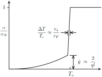
Figure 2: Schematic plot of the attenuation of transverse sound (for q l ≳ 1 ) ql\gtrsim 1) α N subscript 𝛼 𝑁 \alpha_{N} Δ T Δ 𝑇 \Delta T
Just as in the EM case, we consider the case when χ q 2 ≪ ω σ ~ ⟂ much-less-than 𝜒 superscript 𝑞 2 𝜔 subscript ~ 𝜎 perpendicular-to \chi q^{2}\ll\omega\tilde{\sigma}_{\perp} D ret T = ( i ω σ ~ ⟂ ) − 1 subscript superscript 𝐷 𝑇 ret superscript 𝑖 𝜔 subscript ~ 𝜎 perpendicular-to 1 D^{T}_{\rm ret}=(i\omega\tilde{\sigma}_{\perp})^{-1} α 𝛼 \alpha 13 g ~ ~ 𝑔 \tilde{g} τ 𝜏 \tau q 𝑞 q ω 𝜔 \omega τ 𝜏 \tau MYamashita10 τ 𝜏 \tau T 𝑇 T T c subscript 𝑇 𝑐 T_{c} χ q 2 ≪ ω σ ~ ⟂ much-less-than 𝜒 superscript 𝑞 2 𝜔 subscript ~ 𝜎 perpendicular-to \chi q^{2}\ll\omega\tilde{\sigma}_{\perp} q l ≳ 1 greater-than-or-equivalent-to 𝑞 𝑙 1 ql\gtrsim 1 ω σ ~ ⟂ 𝜔 subscript ~ 𝜎 perpendicular-to \omega\tilde{\sigma}_{\perp} ( v s / v F ) k F 2 / m subscript 𝑣 𝑠 subscript 𝑣 𝐹 superscript subscript 𝑘 𝐹 2 𝑚 (v_{s}/v_{F})k_{F}^{2}/m χ q 2 𝜒 superscript 𝑞 2 \chi q^{2} v s / v F ≫ ( q / k F ) 2 much-greater-than subscript 𝑣 𝑠 subscript 𝑣 𝐹 superscript 𝑞 subscript 𝑘 𝐹 2 v_{s}/v_{F}\gg(q/k_{F})^{2} v s / v F ≈ 10 − 3 subscript 𝑣 𝑠 subscript 𝑣 𝐹 superscript 10 3 v_{s}/v_{F}\approx 10^{-3} ( q l ≪ 1 ) much-less-than 𝑞 𝑙 1 (ql\ll 1) ( v s / v F ) q l >> ( q / k F ) 2 much-greater-than subscript 𝑣 𝑠 subscript 𝑣 𝐹 𝑞 𝑙 superscript 𝑞 subscript 𝑘 𝐹 2 (v_{s}/v_{F})ql>>(q/k_{F})^{2}
Finally we can estimate the temperature range Δ T = T c − T Δ 𝑇 subscript 𝑇 𝑐 𝑇 \Delta T=T_{c}-T i ω σ ~ ⟂ 𝑖 𝜔 subscript ~ 𝜎 perpendicular-to i\omega\tilde{\sigma}_{\perp} i ω σ ~ − n s ( T ) / m 𝑖 𝜔 ~ 𝜎 subscript 𝑛 𝑠 𝑇 𝑚 i\omega\tilde{\sigma}-n_{s}(T)/m 14 T c subscript 𝑇 𝑐 T_{c} Im Π s ( 1 ) = Im Π N ( 1 ) / ( 1 + ( n s ( T ) / m ω σ 0 ~ g ~ ) 2 ) Im superscript subscript Π s 1 Im subscript superscript Π 1 N 1 superscript subscript n s T m 𝜔 ~ subscript 𝜎 0 ~ g 2 \rm{Im}\Pi_{s}^{(1)}=\rm{Im}\Pi^{(1)}_{N}/\left(1+(n_{s}(T)/m\omega\tilde{\sigma_{0}}\tilde{g})^{2}\right) Π s , N ( 1 ) subscript superscript Π 1 𝑠 𝑁
\Pi^{(1)}_{s,N} q l ≫ 1 much-greater-than 𝑞 𝑙 1 ql\gg 1 Π ( 1 ) superscript Π 1 \Pi^{(1)} Δ T Δ 𝑇 \Delta T Im Π s ( 1 ) Im superscript subscript Π s 1 \rm{Im}\Pi_{s}^{(1)} n s ( T ) = 2 n ( Δ T / T c ) subscript 𝑛 𝑠 𝑇 2 𝑛 Δ 𝑇 subscript 𝑇 𝑐 n_{s}(T)=2n(\Delta T/T_{c})
Δ T T c ≈ v s v F . Δ 𝑇 subscript 𝑇 𝑐 subscript 𝑣 𝑠 subscript 𝑣 𝐹 {\Delta T\over T_{c}}\approx{v_{s}\over v_{F}}. (15)
We conclude that fermionic spinons
in a fermion
couple to phonons in a way which is identical to electron phonon coupling
in the long wavelength limit. For q l ≫ 1 much-greater-than 𝑞 𝑙 1 ql\gg 1 T c subscript 𝑇 𝑐 T_{c} 15 U ( 1 ) 𝑈 1 U(1)
We thank T. Senthil for helpful comments. PAL acknowledges support by NSF under DMR–0804040. YZ is supported by NSFC (No.11074218),
973 Program (No.2011CBA00103), and the Fundamental Research Funds for the Central Universities in China.
References
(1)
Patrick. A. Lee, Science, 321, 1306 (2008)
(2)
Y. Shimizu et al ., Phys. Rev. Lett. 91 , 107001 (2003).
(3)
T. Itou em et al., Phys. Rev. B 77 104413 (2008).
(4)
S. Yamashita et al. , Nature Physics 4 , 459 (2008); preprint.
(5)
M. Yamashita et al ., Nature Phys. 5 , 44 (2009).
(6)
M. Yamashita et al ., Science 328 , 1246 (2010).
(7)
O. Motrunich, Phys. Rev. B 72 , 045105 (2005).
(8)
Sung-Sik Lee and P.A. Lee, Phys. Rev. Lett. 95 , 036403 (2005).
(9)
R. Manna et al ., Phys. Rev. Lett. 104 , 016403 (2010).
(10)
T. Itou et al ., Nature Phys. 6 , 673 (2010).
(11)
T. Grover et al ., Phys. Rev. B 81 , 245121 (2010).
(12)
J. S. Helton, et. al. , Phys. Rev. Lett. 98 , 107204 (2007).
(13)
Y. Okamoto et al .,, Phys. Rev. Lett. 99 , 137207 (2007).
(14)
D. Mross and T. Senthil, arXiv 1007.2413.
(15)
E. I. Blount, Phys. Rev. 114 , 418 (1959).
(16)
T. Tsuneto, Phys. Rev. 121 , 402 (1961).
(17)
W. P. Mason, Phy. Rev. 97 , 557 (1955).
(18)
R. W. Morse, Phy. Rev. 97 , 1716 (1955).
(19)
A. B. Pippard, Phil. Mag. 41 , 1104 (1955); Proc. R. Soc. London, A257, No. 1289, 165 (1960).
(20)
J.R. Leibowitz, Phys. Rev. 136 , A22 (1964).
(21)
P.A. Lee and N. Nagaosa, Phys. Rev. B 5621 (1992).
I Supplementary Material
I.1 Sound absorption and attenuation in a liquid
Fluid viscosity will cause sound absorption and attenuation in a liquid. To
discuss this effect, we begin with linearlized Navier-Stokes equation,
ρ ∂ 𝐮 ∂ t = − ∇ p + ( 4 3 η + χ ) ∇ ( ∇ ⋅ 𝐮 ) − η ∇ × ∇ × 𝐮 , 𝜌 𝐮 𝑡 ∇ 𝑝 4 3 𝜂 𝜒 ∇ ⋅ ∇ 𝐮 𝜂 ∇ ∇ 𝐮 \rho\frac{\partial\mathbf{u}}{\partial t}=-\nabla p+\left(\frac{4}{3}\eta+\chi\right)\nabla\left(\nabla\cdot\mathbf{u}\right)-\eta\nabla\times\nabla\times\mathbf{u,} (16)
where ρ 𝜌 \rho 𝐮 𝐮 \mathbf{u} p 𝑝 p η 𝜂 \eta χ 𝜒 \chi ρ 𝜌 \rho ρ = ρ 0 ( 1 + s ) 𝜌 subscript 𝜌 0 1 𝑠 \rho=\rho_{0}\left(1+s\right) s 𝑠 s ρ 0 subscript 𝜌 0 \rho_{0}
∇ ⋅ 𝐮 = − ∂ s ∂ t . ⋅ ∇ 𝐮 𝑠 𝑡 \nabla\cdot\mathbf{u}=-\frac{\partial s}{\partial t}. (17)
The acoustic pressure p 𝑝 p
p = ( ∂ p ∂ ρ ) ρ 0 ρ 0 s = ρ 0 v s 2 s 𝑝 subscript 𝑝 𝜌 subscript 𝜌 0 subscript 𝜌 0 𝑠 subscript 𝜌 0 superscript subscript 𝑣 𝑠 2 𝑠 p=\left(\frac{\partial p}{\partial\rho}\right)_{\rho_{0}}\rho_{0}s=\rho_{0}v_{s}^{2}s (18)
in terms of s 𝑠 s v s subscript 𝑣 𝑠 v_{s}
( 1 + τ s ∂ ∂ t ) ∇ 2 p = 1 v s 2 ∂ 2 p ∂ t 2 , 1 subscript 𝜏 𝑠 𝑡 superscript ∇ 2 𝑝 1 superscript subscript 𝑣 𝑠 2 superscript 2 𝑝 superscript 𝑡 2 \left(1+\tau_{s}\frac{\partial}{\partial t}\right)\nabla^{2}p=\frac{1}{v_{s}^{2}}\frac{\partial^{2}p}{\partial t^{2}}, (19)
with a relaxation time given by Eqs.(10). If we assume monofrequency motion,
the above wave quations is reduced to a lossy Helmholtz equation
∇ 2 p + k 2 p = 0 , superscript ∇ 2 𝑝 superscript 𝑘 2 𝑝 0 \nabla^{2}p+k^{2}p=0, (20)
where k = ω v s 1 ( 1 + i ω τ s ) 1 / 2 𝑘 𝜔 subscript 𝑣 𝑠 1 superscript 1 𝑖 𝜔 subscript 𝜏 𝑠 1 2 k=\frac{\omega}{v_{s}}\frac{1}{\left(1+i\omega\tau_{s}\right)^{1/2}} α = − 𝛼 \alpha=- k 𝑘 k
α = 1 2 ω v s [ 1 + ( ω τ s ) 2 − 1 1 + ( ω τ s ) 2 ] 1 / 2 . 𝛼 1 2 𝜔 subscript 𝑣 𝑠 superscript delimited-[] 1 superscript 𝜔 subscript 𝜏 𝑠 2 1 1 superscript 𝜔 subscript 𝜏 𝑠 2 1 2 \alpha=\frac{1}{\sqrt{2}}\frac{\omega}{v_{s}}\left[\frac{\sqrt{1+\left(\omega\tau_{s}\right)^{2}}-1}{1+\left(\omega\tau_{s}\right)^{2}}\right]^{1/2}. (21)
In the limit ω τ s ≪ 1 much-less-than 𝜔 subscript 𝜏 𝑠 1 \omega\tau_{s}\ll 1
I.2 Screened spinon phonon coupling for longitudinal mode
Without the loss of generality, the spinon phonon coupling M 𝐤 λ ( 𝐪 ) subscript 𝑀 𝐤 𝜆 𝐪 M_{\mathbf{k}\lambda}\left(\mathbf{q}\right)
M 𝐤 λ ( 𝐪 ) = 1 3 f ( k , q ) + ∑ l ≥ 1 , m a l m Y l m ( θ , ϕ ) , subscript 𝑀 𝐤 𝜆 𝐪 1 3 𝑓 𝑘 𝑞 subscript 𝑙 1 𝑚
subscript 𝑎 𝑙 𝑚 subscript 𝑌 𝑙 𝑚 𝜃 italic-ϕ M_{\mathbf{k}\lambda}\left(\mathbf{q}\right)=\frac{1}{3}f(k,q)+\sum\limits_{l\geq 1,m}a_{lm}Y_{lm}\left(\theta,\phi\right), (22)
where f ( k , q ) = k 2 q m 2 ρ i o n ω 𝐪 λ 𝑓 𝑘 𝑞 superscript 𝑘 2 𝑞 𝑚 2 subscript 𝜌 𝑖 𝑜 𝑛 subscript 𝜔 𝐪 𝜆 f(k,q)=\frac{k^{2}q}{m\sqrt{2\rho_{ion}\omega_{\mathbf{q}\lambda}}} θ 𝜃 \theta 𝐤 𝐤 \mathbf{k} 𝐪 𝐪 \mathbf{q} ϕ italic-ϕ \phi 𝐤 𝐤 \mathbf{k} k TF − 1 superscript subscript 𝑘 TF 1 k_{\text{TF}}^{-1} q − 1 superscript 𝑞 1 q^{-1} 1 3 f ( k , q ) 1 3 𝑓 𝑘 𝑞 \frac{1}{3}f(k,q) M ~ 𝐤 λ ( 𝐪 , ω ) subscript ~ 𝑀 𝐤 𝜆 𝐪 𝜔 \tilde{M}_{\mathbf{k}\lambda}\left(\mathbf{q},\omega\right) 22 v s / v F subscript 𝑣 𝑠 subscript 𝑣 𝐹 v_{s}/v_{F}
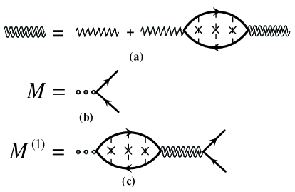
Figure 3: (a) Screening effect of spinon density-density interaction U 𝑈 U U ( 0 ) superscript 𝑈 0 U^{(0)} U 𝑈 U P 𝑃 P
We firstly consider screening effect of the bare spinon density-density
interaction U ( 0 ) ( 𝐪 , ω ) superscript 𝑈 0 𝐪 𝜔 U^{(0)}\left(\mathbf{q},\omega\right)
U ( 𝐪 , ω ) = U ( 0 ) ( 𝐪 , ω ) 1 − P ( 𝐪 , ω ) U ( 0 ) ( 𝐪 , ω ) , 𝑈 𝐪 𝜔 superscript 𝑈 0 𝐪 𝜔 1 𝑃 𝐪 𝜔 superscript 𝑈 0 𝐪 𝜔 U\left(\mathbf{q},\omega\right)=\frac{U^{\left(0\right)}\left(\mathbf{q},\omega\right)}{1-P\left(\mathbf{q},\omega\right)U^{\left(0\right)}\left(\mathbf{q},\omega\right)}, (23)
where P 𝑃 P U 𝑈 U M ~ 𝐤 λ ( 𝐪 , ω ) subscript ~ 𝑀 𝐤 𝜆 𝐪 𝜔 \tilde{M}_{\mathbf{k}\lambda}\left(\mathbf{q},\omega\right)
M ~ 𝐤 λ ( 𝐪 , ω ) = M 𝐤 λ ( 𝐪 ) + M 𝐤 λ ( 1 ) ( 𝐪 , ω ) , subscript ~ 𝑀 𝐤 𝜆 𝐪 𝜔 subscript 𝑀 𝐤 𝜆 𝐪 superscript subscript 𝑀 𝐤 𝜆 1 𝐪 𝜔 \tilde{M}_{\mathbf{k}\lambda}\left(\mathbf{q},\omega\right)=M_{\mathbf{k}\lambda}\left(\mathbf{q}\right)+M_{\mathbf{k}\lambda}^{(1)}\left(\mathbf{q},\omega\right), (24)
where M 𝐤 λ ( 1 ) superscript subscript 𝑀 𝐤 𝜆 1 M_{\mathbf{k}\lambda}^{(1)}
M 𝐤 λ ( 1 ) ( 𝐪 , i ω n ) = 2 β ∑ i k m , 𝐤 M 𝐤 λ ( 𝐪 ) 𝒢 ( 𝐤 + 𝐪 , i k m ) 𝒢 ( 𝐤 , i ω n + i k m ) U ( 𝐪 , i ω n ) γ ( 𝐪 , 𝐤 , i k m , i ω n + i k m ) , superscript subscript 𝑀 𝐤 𝜆 1 𝐪 𝑖 subscript 𝜔 𝑛 2 𝛽 subscript 𝑖 subscript 𝑘 𝑚 𝐤
subscript 𝑀 𝐤 𝜆 𝐪 𝒢 𝐤 𝐪 𝑖 subscript 𝑘 𝑚 𝒢 𝐤 𝑖 subscript 𝜔 𝑛 𝑖 subscript 𝑘 𝑚 𝑈 𝐪 𝑖 subscript 𝜔 𝑛 𝛾 𝐪 𝐤 𝑖 subscript 𝑘 𝑚 𝑖 subscript 𝜔 𝑛 𝑖 subscript 𝑘 𝑚 M_{\mathbf{k}\lambda}^{(1)}\left(\mathbf{q},i\omega_{n}\right)=\frac{2}{\beta}\sum_{ik_{m},\mathbf{k}}M_{\mathbf{k}\lambda}\left(\mathbf{q}\right)\mathcal{G}\left(\mathbf{k+q},ik_{m}\right)\mathcal{G}\left(\mathbf{k},i\omega_{n}+ik_{m}\right)U\left(\mathbf{q},i\omega_{n}\right)\gamma\left(\mathbf{q},\mathbf{k},ik_{m},i\omega_{n}+ik_{m}\right), (25)
as shown in Fig.3(c). The vertex function γ 𝛾 \gamma
γ ( 𝐪 , 𝐤 , i k m , i ω n + i k m ) 𝛾 𝐪 𝐤 𝑖 subscript 𝑘 𝑚 𝑖 subscript 𝜔 𝑛 𝑖 subscript 𝑘 𝑚 \displaystyle\gamma\left(\mathbf{q,k},ik_{m},i\omega_{n}+ik_{m}\right) = \displaystyle= 1 + n i m p ∑ 𝐤 ′ 𝒢 ( 𝐤 ′ + 𝐪 , i k m ) 𝒢 ( 𝐤 ′ , i ω n + i k m ) 1 subscript 𝑛 𝑖 𝑚 𝑝 subscript superscript 𝐤 ′ 𝒢 superscript 𝐤 ′ 𝐪 𝑖 subscript 𝑘 𝑚 𝒢 superscript 𝐤 ′ 𝑖 subscript 𝜔 𝑛 𝑖 subscript 𝑘 𝑚 \displaystyle 1+n_{imp}\sum_{\mathbf{k}^{\prime}}\mathcal{G}\left(\mathbf{k}^{\prime}\mathbf{+q},ik_{m}\right)\mathcal{G}\left(\mathbf{k}^{\prime},i\omega_{n}+ik_{m}\right) (26)
× T 𝐤 + 𝐪 , 𝐤 ′ + 𝐪 ( i k m ) T 𝐤 ′ 𝐤 ( i ω n + i k m ) γ ( 𝐪 , 𝐤 ′ , i k m , i ω n + i k m ) , absent subscript 𝑇 𝐤 𝐪 superscript 𝐤 ′ 𝐪
𝑖 subscript 𝑘 𝑚 subscript 𝑇 superscript 𝐤 ′ 𝐤 𝑖 subscript 𝜔 𝑛 𝑖 subscript 𝑘 𝑚 𝛾 𝐪 superscript 𝐤 ′ 𝑖 subscript 𝑘 𝑚 𝑖 subscript 𝜔 𝑛 𝑖 subscript 𝑘 𝑚 \displaystyle\times T_{\mathbf{k+q,k}^{\prime}\mathbf{+q}}\left(ik_{m}\right)T_{\mathbf{k}^{\prime}\mathbf{k}}\left(i\omega_{n}+ik_{m}\right)\gamma\left(\mathbf{q,k}^{\prime},ik_{m},i\omega_{n}+ik_{m}\right),
where T 𝐤 ′ 𝐤 subscript 𝑇 superscript 𝐤 ′ 𝐤 T_{\mathbf{k}^{\prime}\mathbf{k}} n i m p subscript 𝑛 𝑖 𝑚 𝑝 n_{imp}
To proceed we shall make use of the following approximations,
𝒢 adv ( 𝐤 + 𝐪 , ϵ ) 𝒢 ret ( 𝐤 , ϵ + ω ) subscript 𝒢 adv 𝐤 𝐪 italic-ϵ subscript 𝒢 ret 𝐤 italic-ϵ 𝜔 \displaystyle\mathcal{G}_{\text{adv}}\left(\mathbf{k+q},\epsilon\right)\mathcal{G}_{\text{ret}}\left(\mathbf{k},\epsilon+\omega\right) ≃ similar-to-or-equals \displaystyle\simeq 2 i π δ ( ϵ − ξ 𝐤 ) q v F cos θ + ω + i / τ , 2 𝑖 𝜋 𝛿 italic-ϵ subscript 𝜉 𝐤 𝑞 subscript 𝑣 𝐹 𝜃 𝜔 𝑖 𝜏 \displaystyle\frac{2i\pi\delta\left(\epsilon-\xi_{\mathbf{k}}\right)}{qv_{F}\cos\theta+\omega+i/\tau}, (27)
∫ d ϵ 2 π i n F ( ϵ ) 𝒢 ret ( 𝐤 + 𝐪 , ϵ ) 𝒢 ret ( 𝐤 , ϵ + ω ) 𝑑 italic-ϵ 2 𝜋 𝑖 subscript 𝑛 𝐹 italic-ϵ subscript 𝒢 ret 𝐤 𝐪 italic-ϵ subscript 𝒢 ret 𝐤 italic-ϵ 𝜔 \displaystyle\int\frac{d\epsilon}{2\pi i}n_{F}\left(\epsilon\right)\mathcal{G}_{\text{ret}}\left(\mathbf{k+q},\epsilon\right)\mathcal{G}_{\text{ret}}\left(\mathbf{k},\epsilon+\omega\right) ≃ similar-to-or-equals \displaystyle\simeq − ∂ n F ( ξ 𝐤 ) ∂ ξ 𝐤 , subscript 𝑛 𝐹 subscript 𝜉 𝐤 subscript 𝜉 𝐤 \displaystyle-\frac{\partial n_{F}\left(\xi_{\mathbf{k}}\right)}{\partial\xi_{\mathbf{k}}}, (28)
∫ d ϵ 2 π i n F ( ϵ ) 𝒢 adv ( 𝐤 + 𝐪 , ϵ ) 𝒢 adv ( 𝐤 , ϵ − ω ) 𝑑 italic-ϵ 2 𝜋 𝑖 subscript 𝑛 𝐹 italic-ϵ subscript 𝒢 adv 𝐤 𝐪 italic-ϵ subscript 𝒢 adv 𝐤 italic-ϵ 𝜔 \displaystyle\int\frac{d\epsilon}{2\pi i}n_{F}\left(\epsilon\right)\mathcal{G}_{\text{adv}}\left(\mathbf{k+q},\epsilon\right)\mathcal{G}_{\text{adv}}\left(\mathbf{k},\epsilon-\omega\right) ≃ similar-to-or-equals \displaystyle\simeq ∂ n F ( ξ 𝐤 ) ∂ ξ 𝐤 . subscript 𝑛 𝐹 subscript 𝜉 𝐤 subscript 𝜉 𝐤 \displaystyle\frac{\partial n_{F}\left(\xi_{\mathbf{k}}\right)}{\partial\xi_{\mathbf{k}}}. (29)
For l ≥ 1 𝑙 1 l\geq 1
∫ 𝑑 Ω Y l m ( θ , ϕ ) ∫ d ϵ 2 π i n F ( ϵ ) 𝒢 ret(adv) ( 𝐤 + 𝐪 , ϵ ) 𝒢 ret(adv) ( 𝐤 , ϵ + ω ) = 0 . differential-d Ω subscript 𝑌 𝑙 𝑚 𝜃 italic-ϕ 𝑑 italic-ϵ 2 𝜋 𝑖 subscript 𝑛 𝐹 italic-ϵ subscript 𝒢 ret(adv) 𝐤 𝐪 italic-ϵ subscript 𝒢 ret(adv) 𝐤 italic-ϵ 𝜔 0 \int d\Omega Y_{lm}\left(\theta,\phi\right)\int\frac{d\epsilon}{2\pi i}n_{F}\left(\epsilon\right)\mathcal{G}_{\text{ret(adv)}}\left(\mathbf{k+q},\epsilon\right)\mathcal{G}_{\text{ret(adv)}}\left(\mathbf{k},\epsilon+\omega\right)=0. (30)
With the help of optical sum rule and using the relation
1 2 τ = − n i m p Im T 𝐤𝐤 , 1 2 𝜏 subscript 𝑛 𝑖 𝑚 𝑝 Im subscript 𝑇 𝐤𝐤 \frac{1}{2\tau}=-n_{imp}\text{Im}T_{\mathbf{kk}},
we find that
γ 1 ( 𝐪 , 𝐤 , ϵ , ϵ + ω ) subscript 𝛾 1 𝐪 𝐤 italic-ϵ italic-ϵ 𝜔 \displaystyle\gamma_{1}\left(\mathbf{q,k},\epsilon,\epsilon+\omega\right) ≡ \displaystyle\equiv γ ( 𝐪 , 𝐤 , ϵ − i η , ϵ + ω + i η ) = 1 1 + s 0 ( a ) / a , 𝛾 𝐪 𝐤 italic-ϵ 𝑖 𝜂 italic-ϵ 𝜔 𝑖 𝜂 1 1 subscript 𝑠 0 𝑎 𝑎 \displaystyle\gamma\left(\mathbf{q,k},\epsilon-i\eta,\epsilon+\omega+i\eta\right)=\frac{1}{1+s_{0}\left(a\right)/a}, (31)
γ 2 ( 𝐪 , 𝐤 , ϵ , ϵ + ω ) subscript 𝛾 2 𝐪 𝐤 italic-ϵ italic-ϵ 𝜔 \displaystyle\gamma_{2}\left(\mathbf{q,k},\epsilon,\epsilon+\omega\right) ≡ \displaystyle\equiv γ ( 𝐪 , 𝐤 , ϵ + i η , ϵ + ω + i η ) = 1 , 𝛾 𝐪 𝐤 italic-ϵ 𝑖 𝜂 italic-ϵ 𝜔 𝑖 𝜂 1 \displaystyle\gamma\left(\mathbf{q,k},\epsilon+i\eta,\epsilon+\omega+i\eta\right)=1, (32)
where a = q l / ( 1 + i ω τ ) 𝑎 𝑞 𝑙 1 𝑖 𝜔 𝜏 a=ql/(1+i\omega\tau) ω τ = v s v F q l ≪ 1 𝜔 𝜏 subscript 𝑣 𝑠 subscript 𝑣 𝐹 𝑞 𝑙 much-less-than 1 \omega\tau=\frac{v_{s}}{v_{F}}ql\ll 1 a = q l 𝑎 𝑞 𝑙 a=ql P 𝑃 P
P ( 𝐪 , i ω n ) = ∑ 𝐤 ∑ i k m 𝒢 ( 𝐤 + 𝐪 , i k m ) 𝒢 ( 𝐤 , i ω n + i k m ) γ ( 𝐪 , 𝐤 , i k m , i ω n + i k m ) , 𝑃 𝐪 𝑖 subscript 𝜔 𝑛 subscript 𝐤 subscript 𝑖 subscript 𝑘 𝑚 𝒢 𝐤 𝐪 𝑖 subscript 𝑘 𝑚 𝒢 𝐤 𝑖 subscript 𝜔 𝑛 𝑖 subscript 𝑘 𝑚 𝛾 𝐪 𝐤 𝑖 subscript 𝑘 𝑚 𝑖 subscript 𝜔 𝑛 𝑖 subscript 𝑘 𝑚 P\left(\mathbf{q},i\omega_{n}\right)=\sum_{\mathbf{k}}\sum_{ik_{m}}\mathcal{G}\left(\mathbf{k+q},ik_{m}\right)\mathcal{G}\left(\mathbf{k},i\omega_{n}+ik_{m}\right)\gamma\left(\mathbf{q,k},ik_{m},i\omega_{n}+ik_{m}\right), (33)
Taking analytical continuation, we have
P ( 𝐪 , ω ) 𝑃 𝐪 𝜔 \displaystyle P\left(\mathbf{q},\omega\right) = \displaystyle= 2 i ∑ 𝐤 ∫ − ∞ ∞ d ϵ 2 π n F ( ϵ ) γ 2 ( 𝐪 , 𝐤 , ϵ , ϵ + ω ) 2 𝑖 subscript 𝐤 superscript subscript 𝑑 italic-ϵ 2 𝜋 subscript 𝑛 𝐹 italic-ϵ subscript 𝛾 2 𝐪 𝐤 italic-ϵ italic-ϵ 𝜔 \displaystyle 2i\sum_{\mathbf{k}}\int_{-\infty}^{\infty}\frac{d\epsilon}{2\pi}n_{F}\left(\epsilon\right)\gamma_{2}\left(\mathbf{q,k},\epsilon,\epsilon+\omega\right) (34)
× [ 𝒢 ret ( 𝐤 , ϵ + ω ) 𝒢 ret ( 𝐤 + 𝐪 , ϵ ) − 𝒢 adv ( 𝐤 + 𝐪 , ϵ − ω ) 𝒢 adv ( 𝐤 , ϵ ) ] absent delimited-[] subscript 𝒢 ret 𝐤 italic-ϵ 𝜔 subscript 𝒢 ret 𝐤 𝐪 italic-ϵ subscript 𝒢 adv 𝐤 𝐪 italic-ϵ 𝜔 subscript 𝒢 adv 𝐤 italic-ϵ \displaystyle\times\left[\mathcal{G}_{\text{ret}}\left(\mathbf{k},\epsilon+\omega\right)\mathcal{G}_{\text{ret}}\left(\mathbf{k+q},\epsilon\right)-\mathcal{G}_{\text{adv}}\left(\mathbf{k+q},\epsilon-\omega\right)\mathcal{G}_{\text{adv}}\left(\mathbf{k},\epsilon\right)\right]
+ 2 i ∑ 𝐤 ∫ − ∞ ∞ d ϵ 2 π n F ( ϵ ) γ 1 ( 𝐪 , 𝐤 , ϵ , ϵ + ω ) 2 𝑖 subscript 𝐤 superscript subscript 𝑑 italic-ϵ 2 𝜋 subscript 𝑛 𝐹 italic-ϵ subscript 𝛾 1 𝐪 𝐤 italic-ϵ italic-ϵ 𝜔 \displaystyle+2i\sum_{\mathbf{k}}\int_{-\infty}^{\infty}\frac{d\epsilon}{2\pi}n_{F}\left(\epsilon\right)\gamma_{1}\left(\mathbf{q,k},\epsilon,\epsilon+\omega\right)
× [ − 𝒢 ret ( 𝐤 , ϵ + ω ) 𝒢 adv ( 𝐤 + 𝐪 , ϵ ) + 𝒢 adv ( 𝐤 + 𝐪 , ϵ − ω ) 𝒢 ret ( 𝐤 , ϵ ) ] absent delimited-[] subscript 𝒢 ret 𝐤 italic-ϵ 𝜔 subscript 𝒢 adv 𝐤 𝐪 italic-ϵ subscript 𝒢 adv 𝐤 𝐪 italic-ϵ 𝜔 subscript 𝒢 ret 𝐤 italic-ϵ \displaystyle\times\left[-\mathcal{G}_{\text{ret}}\left(\mathbf{k},\epsilon+\omega\right)\mathcal{G}_{\text{adv}}\left(\mathbf{k+q},\epsilon\right)+\mathcal{G}_{\text{adv}}\left(\mathbf{k+q},\epsilon-\omega\right)\mathcal{G}_{\text{ret}}\left(\mathbf{k},\epsilon\right)\right]
= \displaystyle= − N ( 0 ) [ 1 − i ω τ s 0 ( a ) / a 1 + s 0 ( a ) / a ] , 𝑁 0 delimited-[] 1 𝑖 𝜔 𝜏 subscript 𝑠 0 𝑎 𝑎 1 subscript 𝑠 0 𝑎 𝑎 \displaystyle-N\left(0\right)\left[1-i\omega\tau\frac{s_{0}\left(a\right)/a}{1+s_{0}\left(a\right)/a}\right],
When the Thomas Fermi screening length k TF − 1 ≪ q − 1 much-less-than superscript subscript 𝑘 TF 1 superscript 𝑞 1 k_{\text{TF}}^{-1}\ll q^{-1} N ( 0 ) U ( 0 ) ( 𝐪 , ω ) ≫ 1 much-greater-than 𝑁 0 superscript 𝑈 0 𝐪 𝜔 1 N\left(0\right)U^{\left(0\right)}\left(\mathbf{q},\omega\right)\gg 1 U ( 𝐪 , ω ) 𝑈 𝐪 𝜔 U\left(\mathbf{q},\omega\right)
U ( 𝐪 , ω ) = 1 N ( 0 ) [ 1 − i ω τ s 0 ( a ) / a 1 + s 0 ( a ) / a ] . 𝑈 𝐪 𝜔 1 𝑁 0 delimited-[] 1 𝑖 𝜔 𝜏 subscript 𝑠 0 𝑎 𝑎 1 subscript 𝑠 0 𝑎 𝑎 U\left(\mathbf{q},\omega\right)=\frac{1}{N\left(0\right)\left[1-i\omega\tau\frac{s_{0}\left(a\right)/a}{1+s_{0}\left(a\right)/a}\right]}. (35)
Then we are ready to calculate M 𝐤 λ ( 1 ) ( 𝐪 ) superscript subscript 𝑀 𝐤 𝜆 1 𝐪 M_{\mathbf{k}\lambda}^{(1)}\left(\mathbf{q}\right)
M 𝐤 λ ( 1 ) ( 𝐪 , ω ) superscript subscript 𝑀 𝐤 𝜆 1 𝐪 𝜔 \displaystyle M_{\mathbf{k}\lambda}^{(1)}\left(\mathbf{q},\omega\right) = \displaystyle= 2 β ∑ 𝐤 M 𝐤 λ ( 𝐪 ) ∑ i k m 𝒢 ( 𝐤 + 𝐪 , i k m ) 𝒢 ( 𝐤 , i ω n + i k m ) γ U ( 𝐪 , i ω n ) 2 𝛽 subscript 𝐤 subscript 𝑀 𝐤 𝜆 𝐪 subscript 𝑖 subscript 𝑘 𝑚 𝒢 𝐤 𝐪 𝑖 subscript 𝑘 𝑚 𝒢 𝐤 𝑖 subscript 𝜔 𝑛 𝑖 subscript 𝑘 𝑚 𝛾 𝑈 𝐪 𝑖 subscript 𝜔 𝑛 \displaystyle\frac{2}{\beta}\sum_{\mathbf{k}}M_{\mathbf{k}\lambda}\left(\mathbf{q}\right)\sum_{ik_{m}}\mathcal{G}\left(\mathbf{k+q},ik_{m}\right)\mathcal{G}\left(\mathbf{k},i\omega_{n}+ik_{m}\right)\gamma U\left(\mathbf{q},i\omega_{n}\right) (36)
= \displaystyle= 1 3 f ( k , q ) P ( 𝐪 , ω ) U ( 𝐪 , ω ) − 2 i ω f ( k , q ) ∑ 𝐤 ( cos 2 θ − 1 3 ) 1 3 𝑓 𝑘 𝑞 𝑃 𝐪 𝜔 𝑈 𝐪 𝜔 2 𝑖 𝜔 𝑓 𝑘 𝑞 subscript 𝐤 superscript 2 𝜃 1 3 \displaystyle\frac{1}{3}f\left(k,q\right)P\left(\mathbf{q},\omega\right)U\left(\mathbf{q},\omega\right)-2i\omega f\left(k,q\right)\sum_{\mathbf{k}}\left(\cos^{2}\theta-\frac{1}{3}\right)
× ∫ − ∞ ∞ d ϵ 2 π [ − ∂ n F ( ϵ ) ∂ ϵ ] 𝒢 ret ( 𝐤 , ϵ + ω ) 𝒢 adv ( 𝐤 + 𝐪 , ϵ ) γ 1 U ( 𝐪 , ω ) \displaystyle\times\int_{-\infty}^{\infty}\frac{d\epsilon}{2\pi}\left[-\frac{\partial n_{F}\left(\epsilon\right)}{\partial\epsilon}\right]\mathcal{G}_{\text{ret}}\left(\mathbf{k},\epsilon+\omega\right)\mathcal{G}_{\text{adv}}\left(\mathbf{k+q},\epsilon\right)\gamma_{1}U\left(\mathbf{q},\omega\right)
= \displaystyle= f ( k , q ) [ − 1 3 + i ω τ a s 2 ( a ) − s 0 ( a ) / 3 1 + ( 1 − i ω τ ) s 0 ( a ) / a ] 𝑓 𝑘 𝑞 delimited-[] 1 3 𝑖 𝜔 𝜏 𝑎 subscript 𝑠 2 𝑎 subscript 𝑠 0 𝑎 3 1 1 𝑖 𝜔 𝜏 subscript 𝑠 0 𝑎 𝑎 \displaystyle f\left(k,q\right)\left[-\frac{1}{3}+i\frac{\omega\tau}{a}\frac{s_{2}\left(a\right)-s_{0}\left(a\right)/3}{1+\left(1-i\omega\tau\right)s_{0}\left(a\right)/a}\right]
Therefore
M ~ 𝐤 λ ( 𝐪 ) = k 2 q m 2 ρ i o n ω 𝐪 λ [ cos 2 θ − 1 3 + i v s v F s 2 ( a ) − s 0 ( a ) / 3 1 + ( 1 − i ω τ ) s 0 ( a ) / a ] . subscript ~ 𝑀 𝐤 𝜆 𝐪 superscript 𝑘 2 𝑞 𝑚 2 subscript 𝜌 𝑖 𝑜 𝑛 subscript 𝜔 𝐪 𝜆 delimited-[] superscript 2 𝜃 1 3 𝑖 subscript 𝑣 𝑠 subscript 𝑣 𝐹 subscript 𝑠 2 𝑎 subscript 𝑠 0 𝑎 3 1 1 𝑖 𝜔 𝜏 subscript 𝑠 0 𝑎 𝑎 \tilde{M}_{\mathbf{k}\lambda}\left(\mathbf{q}\right)=\frac{k^{2}q}{m\sqrt{2\rho_{ion}\omega_{\mathbf{q}\lambda}}}\left[\cos^{2}\theta-\frac{1}{3}+i\frac{v_{s}}{v_{F}}\frac{s_{2}\left(a\right)-s_{0}\left(a\right)/3}{1+\left(1-i\omega\tau\right)s_{0}\left(a\right)/a}\right].
Thus we can calculate the sound attenuation constant through the unscreened
bubble [Fig1.(a)] with the traceless coupling matrix,
M ~ 𝐤 λ ( 𝐪 ) = ( 𝐤 ⋅ 𝐪 ) ( 𝐤 ⋅ ε ^ 𝐪 λ ) − 1 3 k 2 ( 𝐪 ⋅ ε ^ 𝐪 λ ) m 2 ρ i o n ω 𝐪 λ + O ( v s v F ) , subscript ~ 𝑀 𝐤 𝜆 𝐪 ⋅ 𝐤 𝐪 ⋅ 𝐤 subscript ^ 𝜀 𝐪 𝜆 1 3 superscript 𝑘 2 ⋅ 𝐪 subscript ^ 𝜀 𝐪 𝜆 𝑚 2 subscript 𝜌 𝑖 𝑜 𝑛 subscript 𝜔 𝐪 𝜆 𝑂 subscript 𝑣 𝑠 subscript 𝑣 𝐹 \tilde{M}_{\mathbf{k}\lambda}\left(\mathbf{q}\right)=\frac{\left(\mathbf{k}\cdot\mathbf{q}\right)\left(\mathbf{k}\cdot\hat{\varepsilon}_{\mathbf{q}\lambda}\right)-\frac{1}{3}k^{2}\left(\mathbf{q}\cdot\hat{\varepsilon}_{\mathbf{q}\lambda}\right)}{m\sqrt{2\rho_{ion}\omega_{\mathbf{q}\lambda}}}+O\left(\frac{v_{s}}{v_{F}}\right), (37)
for longitudinal mode.
I.3 Longitudinal sound attenuation
Then we calculate longitudinal sound attenuation constant using the above
spinon phonon coupling. In this case, we can express Π ( 𝐪 , i ω n ) Π 𝐪 𝑖 subscript 𝜔 𝑛 \Pi\left(\mathbf{q},i\omega_{n}\right) Γ ( 𝐪 , 𝐤 , i k m , i ω n + i k m ) Γ 𝐪 𝐤 𝑖 subscript 𝑘 𝑚 𝑖 subscript 𝜔 𝑛 𝑖 subscript 𝑘 𝑚 \Gamma\left(\mathbf{q,k},ik_{m},i\omega_{n}+ik_{m}\right)
Π ( 𝐪 , i ω n ) = 2 β ∑ 𝐤 M ~ 𝐤 λ ( 𝐪 ) ∑ i k m 𝒢 ( 𝐤 + 𝐪 , i k m ) 𝒢 ( 𝐤 , i ω n + i k m ) Γ ( 𝐪 , 𝐤 , i k m , i ω n + i k m ) , Π 𝐪 𝑖 subscript 𝜔 𝑛 2 𝛽 subscript 𝐤 subscript ~ 𝑀 𝐤 𝜆 𝐪 subscript 𝑖 subscript 𝑘 𝑚 𝒢 𝐤 𝐪 𝑖 subscript 𝑘 𝑚 𝒢 𝐤 𝑖 subscript 𝜔 𝑛 𝑖 subscript 𝑘 𝑚 Γ 𝐪 𝐤 𝑖 subscript 𝑘 𝑚 𝑖 subscript 𝜔 𝑛 𝑖 subscript 𝑘 𝑚 \Pi\left(\mathbf{q},i\omega_{n}\right)=\frac{2}{\beta}\sum_{\mathbf{k}}\tilde{M}_{\mathbf{k}\lambda}\left(\mathbf{q}\right)\sum_{ik_{m}}\mathcal{G}\left(\mathbf{k+q},ik_{m}\right)\mathcal{G}\left(\mathbf{k},i\omega_{n}+ik_{m}\right)\Gamma\left(\mathbf{q,k},ik_{m},i\omega_{n}+ik_{m}\right), (38)
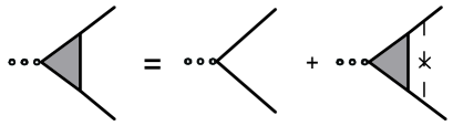
where the vertex function Γ Γ \Gamma
Γ ( 𝐪 , 𝐤 , i k m , i ω n + i k m ) Γ 𝐪 𝐤 𝑖 subscript 𝑘 𝑚 𝑖 subscript 𝜔 𝑛 𝑖 subscript 𝑘 𝑚 \displaystyle\Gamma\left(\mathbf{q,k},ik_{m},i\omega_{n}+ik_{m}\right) = \displaystyle= M ~ 𝐤 λ ( 𝐪 ) + n i m p ∑ 𝐤 ′ 𝒢 ( 𝐤 ′ + 𝐪 , i k m ) 𝒢 ( 𝐤 ′ , i ω n + i k m ) subscript ~ 𝑀 𝐤 𝜆 𝐪 subscript 𝑛 𝑖 𝑚 𝑝 subscript superscript 𝐤 ′ 𝒢 superscript 𝐤 ′ 𝐪 𝑖 subscript 𝑘 𝑚 𝒢 superscript 𝐤 ′ 𝑖 subscript 𝜔 𝑛 𝑖 subscript 𝑘 𝑚 \displaystyle\tilde{M}_{\mathbf{k}\lambda}\left(\mathbf{q}\right)+n_{imp}\sum_{\mathbf{k}^{\prime}}\mathcal{G}\left(\mathbf{k}^{\prime}\mathbf{+q},ik_{m}\right)\mathcal{G}\left(\mathbf{k}^{\prime},i\omega_{n}+ik_{m}\right) (39)
× T 𝐤 + 𝐪 , 𝐤 ′ + 𝐪 ( i k m ) T 𝐤 ′ 𝐤 ( i ω n + i k m ) Γ ( 𝐪 , 𝐤 ′ , i k m , i ω n + i k m ) , absent subscript 𝑇 𝐤 𝐪 superscript 𝐤 ′ 𝐪
𝑖 subscript 𝑘 𝑚 subscript 𝑇 superscript 𝐤 ′ 𝐤 𝑖 subscript 𝜔 𝑛 𝑖 subscript 𝑘 𝑚 Γ 𝐪 superscript 𝐤 ′ 𝑖 subscript 𝑘 𝑚 𝑖 subscript 𝜔 𝑛 𝑖 subscript 𝑘 𝑚 \displaystyle\times T_{\mathbf{k+q,k}^{\prime}\mathbf{+q}}\left(ik_{m}\right)T_{\mathbf{k}^{\prime}\mathbf{k}}\left(i\omega_{n}+ik_{m}\right)\Gamma\left(\mathbf{q,k}^{\prime},ik_{m},i\omega_{n}+ik_{m}\right),
and is shown in Fig.4 diagramatically.
Figure 4: Vertex correction in longitudinal sound, the dash line across the
vertex denotes impurity scattering.
It is more convenient to write the analytical continuations of Γ Γ \Gamma
Γ 1 ( 𝐪 , 𝐤 , ϵ , ϵ + ω ) subscript Γ 1 𝐪 𝐤 italic-ϵ italic-ϵ 𝜔 \displaystyle\Gamma_{1}\left(\mathbf{q,k},\epsilon,\epsilon+\omega\right) ≡ \displaystyle\equiv Γ ( 𝐪 , 𝐤 , ϵ − i η , ϵ + ω + i η ) , Γ 𝐪 𝐤 italic-ϵ 𝑖 𝜂 italic-ϵ 𝜔 𝑖 𝜂 \displaystyle\Gamma\left(\mathbf{q,k},\epsilon-i\eta,\epsilon+\omega+i\eta\right), (40)
Γ 2 ( 𝐪 , 𝐤 , ϵ , ϵ + ω ) subscript Γ 2 𝐪 𝐤 italic-ϵ italic-ϵ 𝜔 \displaystyle\Gamma_{2}\left(\mathbf{q,k},\epsilon,\epsilon+\omega\right) ≡ \displaystyle\equiv Γ ( 𝐪 , 𝐤 , ϵ + i η , ϵ + ω + i η ) . Γ 𝐪 𝐤 italic-ϵ 𝑖 𝜂 italic-ϵ 𝜔 𝑖 𝜂 \displaystyle\Gamma\left(\mathbf{q,k},\epsilon+i\eta,\epsilon+\omega+i\eta\right). (41)
We find out the following two solutions,
Γ 1 ( 𝐪 , 𝐤 , ϵ , ϵ + ω ) subscript Γ 1 𝐪 𝐤 italic-ϵ italic-ϵ 𝜔 \displaystyle\Gamma_{1}\left(\mathbf{q,k},\epsilon,\epsilon+\omega\right) = \displaystyle= M ~ 𝐤 λ ( 𝐪 ) − q k F 2 m 2 ρ i o n ω 𝐪 λ [ s 2 ( a ) − 1 3 s 0 ( a ) ] / a 1 + s 0 ( a ) / a , subscript ~ 𝑀 𝐤 𝜆 𝐪 𝑞 superscript subscript 𝑘 𝐹 2 𝑚 2 subscript 𝜌 𝑖 𝑜 𝑛 subscript 𝜔 𝐪 𝜆 delimited-[] subscript 𝑠 2 𝑎 1 3 subscript 𝑠 0 𝑎 𝑎 1 subscript 𝑠 0 𝑎 𝑎 \displaystyle\tilde{M}_{\mathbf{k}\lambda}\left(\mathbf{q}\right)-\frac{qk_{F}^{2}}{m\sqrt{2\rho_{ion}\omega_{\mathbf{q}\lambda}}}\frac{\left[s_{2}\left(a\right)-\frac{1}{3}s_{0}\left(a\right)\right]/a}{1+s_{0}\left(a\right)/a}, (42)
Γ 2 ( 𝐪 , 𝐤 , ϵ , ϵ + ω ) subscript Γ 2 𝐪 𝐤 italic-ϵ italic-ϵ 𝜔 \displaystyle\Gamma_{2}\left(\mathbf{q,k},\epsilon,\epsilon+\omega\right) = \displaystyle= M ~ 𝐤 λ ( 𝐪 ) . subscript ~ 𝑀 𝐤 𝜆 𝐪 \displaystyle\tilde{M}_{\mathbf{k}\lambda}\left(\mathbf{q}\right). (43)
Thus the retarded phonon polarization function can be calculated as
Π ret ( 𝐪 , ω ) subscript Π ret 𝐪 𝜔 \displaystyle\Pi_{\text{ret}}\left(\mathbf{q},\omega\right) = \displaystyle= 2 i ∑ 𝐤 M ~ 𝐤 λ ( 𝐪 ) ∫ − ∞ ∞ d ϵ 2 π n F ( ϵ ) [ 𝒢 ret ( 𝐤 , ϵ + ω ) 𝒢 ret ( 𝐤 + 𝐪 , ϵ ) Γ 2 ( 𝐪 , 𝐤 , ϵ , ϵ + ω ) \displaystyle 2i\sum_{\mathbf{k}}\tilde{M}_{\mathbf{k}\lambda}\left(\mathbf{q}\right)\int_{-\infty}^{\infty}\frac{d\epsilon}{2\pi}n_{F}\left(\epsilon\right)\left[\mathcal{G}_{\text{ret}}\left(\mathbf{k},\epsilon+\omega\right)\mathcal{G}_{\text{ret}}\left(\mathbf{k+q},\epsilon\right)\Gamma_{2}\left(\mathbf{q,k},\epsilon,\epsilon+\omega\right)\right.
− 𝒢 adv ( 𝐤 + 𝐪 , ϵ − ω ) 𝒢 adv ( 𝐤 , ϵ ) Γ 2 ∗ ( 𝐪 , 𝐤 , ϵ , ϵ + ω ) ] \displaystyle\left.-\mathcal{G}_{\text{adv}}\left(\mathbf{k+q},\epsilon-\omega\right)\mathcal{G}_{\text{adv}}\left(\mathbf{k},\epsilon\right)\Gamma_{2}^{\ast}\left(\mathbf{q,k},\epsilon,\epsilon+\omega\right)\right]
+ 2 i ∑ 𝐤 M ~ 𝐤 λ ( 𝐪 ) ∫ − ∞ ∞ d ϵ 2 π n F ( ϵ ) Γ 1 ( 𝐪 , 𝐤 , ϵ , ϵ + ω ) 2 𝑖 subscript 𝐤 subscript ~ 𝑀 𝐤 𝜆 𝐪 superscript subscript 𝑑 italic-ϵ 2 𝜋 subscript 𝑛 𝐹 italic-ϵ subscript Γ 1 𝐪 𝐤 italic-ϵ italic-ϵ 𝜔 \displaystyle+2i\sum_{\mathbf{k}}\tilde{M}_{\mathbf{k}\lambda}\left(\mathbf{q}\right)\int_{-\infty}^{\infty}\frac{d\epsilon}{2\pi}n_{F}\left(\epsilon\right)\Gamma_{1}\left(\mathbf{q,k},\epsilon,\epsilon+\omega\right)
× [ − 𝒢 ret ( 𝐤 , ϵ + ω ) 𝒢 adv ( 𝐤 + 𝐪 , ϵ ) + 𝒢 adv ( 𝐤 + 𝐪 , ϵ − ω ) 𝒢 ret ( 𝐤 , ϵ ) ] . absent delimited-[] subscript 𝒢 ret 𝐤 italic-ϵ 𝜔 subscript 𝒢 adv 𝐤 𝐪 italic-ϵ subscript 𝒢 adv 𝐤 𝐪 italic-ϵ 𝜔 subscript 𝒢 ret 𝐤 italic-ϵ \displaystyle\times\left[-\mathcal{G}_{\text{ret}}\left(\mathbf{k},\epsilon+\omega\right)\mathcal{G}_{\text{adv}}\left(\mathbf{k+q},\epsilon\right)+\mathcal{G}_{\text{adv}}\left(\mathbf{k+q},\epsilon-\omega\right)\mathcal{G}_{\text{ret}}\left(\mathbf{k},\epsilon\right)\right].
The imaginary part of the terms with Γ 2 subscript Γ 2 \Gamma_{2} Γ 2 ∗ superscript subscript Γ 2 ∗ \Gamma_{2}^{\ast}
Im Π ret ( 𝐪 , ω ) Im subscript Π ret 𝐪 𝜔 \displaystyle\text{Im}\Pi_{\text{ret}}\left(\mathbf{q},\omega\right) = \displaystyle= − 2 ω Re ∑ 𝐤 M ~ 𝐤 λ ( 𝐪 ) ∫ − ∞ ∞ d ϵ 2 π [ − ∂ n F ( ϵ ) ∂ ϵ ] 𝒢 ret ( 𝐤 , ϵ + ω ) 𝒢 adv ( 𝐤 + 𝐪 , ϵ ) Γ 1 ( 𝐪 , 𝐤 , ϵ , ϵ + ω ) 2 𝜔 Re subscript 𝐤 subscript ~ 𝑀 𝐤 𝜆 𝐪 superscript subscript 𝑑 italic-ϵ 2 𝜋 delimited-[] subscript 𝑛 𝐹 italic-ϵ italic-ϵ subscript 𝒢 ret 𝐤 italic-ϵ 𝜔 subscript 𝒢 adv 𝐤 𝐪 italic-ϵ subscript Γ 1 𝐪 𝐤 italic-ϵ italic-ϵ 𝜔 \displaystyle-2\omega\text{Re}\sum_{\mathbf{k}}\tilde{M}_{\mathbf{k}\lambda}\left(\mathbf{q}\right)\int_{-\infty}^{\infty}\frac{d\epsilon}{2\pi}\left[-\frac{\partial n_{F}\left(\epsilon\right)}{\partial\epsilon}\right]\mathcal{G}_{\text{ret}}\left(\mathbf{k},\epsilon+\omega\right)\mathcal{G}_{\text{adv}}\left(\mathbf{k+q},\epsilon\right)\Gamma_{1}\left(\mathbf{q,k},\epsilon,\epsilon+\omega\right) (44)
= \displaystyle= ω N ( 0 ) k F 3 2 m ρ i o n v s Re { s 4 ( a ) − 2 3 s 2 ( a ) + 1 9 s 0 ( a ) − [ s 2 ( a ) − 1 3 s 0 ( a ) ] 2 a + s 0 ( a ) } , 𝜔 𝑁 0 superscript subscript 𝑘 𝐹 3 2 𝑚 subscript 𝜌 𝑖 𝑜 𝑛 subscript 𝑣 𝑠 Re subscript 𝑠 4 𝑎 2 3 subscript 𝑠 2 𝑎 1 9 subscript 𝑠 0 𝑎 superscript delimited-[] subscript 𝑠 2 𝑎 1 3 subscript 𝑠 0 𝑎 2 𝑎 subscript 𝑠 0 𝑎 \displaystyle\frac{\omega N\left(0\right)k_{F}^{3}}{2m\rho_{ion}v_{s}}\text{Re}\left\{s_{4}\left(a\right)-\frac{2}{3}s_{2}\left(a\right)+\frac{1}{9}s_{0}\left(a\right)-\frac{\left[s_{2}\left(a\right)-\frac{1}{3}s_{0}\left(a\right)\right]^{2}}{a+s_{0}\left(a\right)}\right\},
Using the expressions of s n ( a ) subscript 𝑠 𝑛 𝑎 s_{n}\left(a\right)
s 0 ( a ) subscript 𝑠 0 𝑎 \displaystyle s_{0}\left(a\right) = \displaystyle= − tan − 1 a , superscript 1 𝑎 \displaystyle-\tan^{-1}a,
s 2 ( a ) subscript 𝑠 2 𝑎 \displaystyle s_{2}\left(a\right) = \displaystyle= − a − tan − 1 a a 2 , 𝑎 superscript 1 𝑎 superscript 𝑎 2 \displaystyle-\frac{a-\tan^{-1}a}{a^{2}},
s 4 ( a ) subscript 𝑠 4 𝑎 \displaystyle s_{4}\left(a\right) = \displaystyle= − − 3 a + a 3 + 3 tan − 1 a 3 a 4 , 3 𝑎 superscript 𝑎 3 3 superscript 1 𝑎 3 superscript 𝑎 4 \displaystyle-\frac{-3a+a^{3}+3\tan^{-1}a}{3a^{4}},
we obtain the longitudinal sound attenuation constant,
α 𝛼 \displaystyle\alpha = \displaystyle= ω N ( 0 ) k F 3 m ρ i o n v s 2 1 3 q l [ q 2 l 2 tan − 1 ( q l ) q l − tan − 1 ( q l ) − 1 3 ] 𝜔 𝑁 0 superscript subscript 𝑘 𝐹 3 𝑚 subscript 𝜌 𝑖 𝑜 𝑛 superscript subscript 𝑣 𝑠 2 1 3 𝑞 𝑙 delimited-[] superscript 𝑞 2 superscript 𝑙 2 superscript 1 𝑞 𝑙 𝑞 𝑙 superscript 1 𝑞 𝑙 1 3 \displaystyle\frac{\omega N\left(0\right)k_{F}^{3}}{m\rho_{ion}v_{s}^{2}}\frac{1}{3ql}\left[\frac{q^{2}l^{2}\tan^{-1}\left(ql\right)}{ql-\tan^{-1}\left(ql\right)}-\frac{1}{3}\right] (45)
= \displaystyle= n m ρ i o n v s τ [ q 2 l 2 tan − 1 ( q l ) q l − tan − 1 ( q l ) − 1 3 ] , 𝑛 𝑚 subscript 𝜌 𝑖 𝑜 𝑛 subscript 𝑣 𝑠 𝜏 delimited-[] superscript 𝑞 2 superscript 𝑙 2 superscript 1 𝑞 𝑙 𝑞 𝑙 superscript 1 𝑞 𝑙 1 3 \displaystyle\frac{nm}{\rho_{ion}v_{s}\tau}\left[\frac{q^{2}l^{2}\tan^{-1}\left(ql\right)}{ql-\tan^{-1}\left(ql\right)}-\frac{1}{3}\right],
where the density of spinons n = N ( 0 ) k F 2 3 m 𝑛 𝑁 0 superscript subscript 𝑘 𝐹 2 3 𝑚 n=\frac{N\left(0\right)k_{F}^{2}}{3m} 45
Similarly, we obtain the longitudinal sound attenuation constant in 2D by
replacing s n ( a ) subscript 𝑠 𝑛 𝑎 s_{n}\left(a\right) t n ( a ) subscript 𝑡 𝑛 𝑎 t_{n}\left(a\right)
α 𝛼 \displaystyle\alpha = \displaystyle= − ω N ( 0 ) k F 3 m ρ i o n v s 2 Re { t 4 ( a ) − t 2 ( a ) + 1 4 t 0 ( a ) − [ t 2 ( a ) − 1 2 t 0 ( a ) ] 2 a + t 0 ( a ) } 𝜔 𝑁 0 superscript subscript 𝑘 𝐹 3 𝑚 subscript 𝜌 𝑖 𝑜 𝑛 superscript subscript 𝑣 𝑠 2 Re subscript 𝑡 4 𝑎 subscript 𝑡 2 𝑎 1 4 subscript 𝑡 0 𝑎 superscript delimited-[] subscript 𝑡 2 𝑎 1 2 subscript 𝑡 0 𝑎 2 𝑎 subscript 𝑡 0 𝑎 \displaystyle-\frac{\omega N\left(0\right)k_{F}^{3}}{m\rho_{ion}v_{s}^{2}}\text{Re}\left\{t_{4}\left(a\right)-t_{2}\left(a\right)+\frac{1}{4}t_{0}\left(a\right)-\frac{\left[t_{2}\left(a\right)-\frac{1}{2}t_{0}\left(a\right)\right]^{2}}{a+t_{0}\left(a\right)}\right\} (46)
= \displaystyle= n m ρ i o n v s τ [ q 2 l 2 1 − 1 + q 2 l 2 − 1 2 ] . 𝑛 𝑚 subscript 𝜌 𝑖 𝑜 𝑛 subscript 𝑣 𝑠 𝜏 delimited-[] superscript 𝑞 2 superscript 𝑙 2 1 1 superscript 𝑞 2 superscript 𝑙 2 1 2 \displaystyle\frac{nm}{\rho_{ion}v_{s}\tau}\left[\frac{q^{2}l^{2}}{1-\sqrt{1+q^{2}l^{2}}}-\frac{1}{2}\right].
I.4 Transverse sound attenuation in an electron gas
We proceed with transverse sound, where there is no vertex correction
(impurity line across the bubbles) because the vertex is odd in the 𝐤 𝐤 \mathbf{k} 𝐪 𝐪 \mathbf{q} Π ( 0 ) superscript Π 0 \Pi^{(0)}
Π ret ( 0 ) ( 𝐪 , ω ) superscript subscript Π ret 0 𝐪 𝜔 \displaystyle\Pi_{\text{ret}}^{\left(0\right)}\left(\mathbf{q},\omega\right) = \displaystyle= − 2 i ∑ 𝐤 [ M 𝐤 λ ( 𝐪 ) ] 2 ∫ − ∞ ∞ d ϵ 2 π { [ n F ( ϵ ) − n F ( ϵ + ω ) ] 𝒢 ret ( 𝐤 , ϵ + ω ) 𝒢 adv ( 𝐤 + 𝐪 , ϵ ) \displaystyle-2i\sum_{\mathbf{k}}[M_{\mathbf{k}\lambda}\left(\mathbf{q}\right)]^{2}\int_{-\infty}^{\infty}\frac{d\epsilon}{2\pi}\left\{\left[n_{F}\left(\epsilon\right)-n_{F}\left(\epsilon+\omega\right)\right]\mathcal{G}_{\text{ret}}\left(\mathbf{k},\epsilon+\omega\right)\mathcal{G}_{\text{adv}}\left(\mathbf{k+q},\epsilon\right)\right. (47)
− n F ( ϵ ) [ 𝒢 ret ( 𝐤 , ϵ + ω ) 𝒢 ret ( 𝐤 + 𝐪 , ϵ ) − 𝒢 adv ( 𝐤 + 𝐪 , ϵ − ω ) 𝒢 adv ( 𝐤 , ϵ ) ] } . \displaystyle\left.-n_{F}\left(\epsilon\right)[\mathcal{G}_{\text{ret}}\left(\mathbf{k},\epsilon+\omega\right)\mathcal{G}_{\text{ret}}\left(\mathbf{k+q},\epsilon\right)-\mathcal{G}_{\text{adv}}\left(\mathbf{k+q},\epsilon-\omega\right)\mathcal{G}_{\text{adv}}\left(\mathbf{k},\epsilon\right)]\right\}.
Similarly to longitudinal mode, the imaginary part of 𝒢 ret 𝒢 ret subscript 𝒢 ret subscript 𝒢 ret \mathcal{G}_{\text{ret}}\mathcal{G}_{\text{ret}} 𝒢 adv 𝒢 adv subscript 𝒢 adv subscript 𝒢 adv \mathcal{G}_{\text{adv}}\mathcal{G}_{\text{adv}}
Im Π ret ( 0 ) ( 𝐪 , ω ) Im superscript subscript Π ret 0 𝐪 𝜔 \displaystyle\text{Im}\Pi_{\text{ret}}^{\left(0\right)}\left(\mathbf{q},\omega\right) = \displaystyle= − 2 ω Re ∑ 𝐤 [ M 𝐤 λ ( 𝐪 ) ] 2 ∫ − ∞ ∞ d ϵ 2 π [ − ∂ n F ( ϵ ) ∂ ϵ ] 𝒢 ret ( 𝐤 , ϵ + ω ) 𝒢 adv ( 𝐤 + 𝐪 , ϵ ) 2 𝜔 Re subscript 𝐤 superscript delimited-[] subscript 𝑀 𝐤 𝜆 𝐪 2 superscript subscript 𝑑 italic-ϵ 2 𝜋 delimited-[] subscript 𝑛 𝐹 italic-ϵ italic-ϵ subscript 𝒢 ret 𝐤 italic-ϵ 𝜔 subscript 𝒢 adv 𝐤 𝐪 italic-ϵ \displaystyle-2\omega\text{Re}\sum_{\mathbf{k}}[M_{\mathbf{k}\lambda}\left(\mathbf{q}\right)]^{2}\int_{-\infty}^{\infty}\frac{d\epsilon}{2\pi}\left[-\frac{\partial n_{F}\left(\epsilon\right)}{\partial\epsilon}\right]\mathcal{G}_{\text{ret}}\left(\mathbf{k},\epsilon+\omega\right)\mathcal{G}_{\text{adv}}\left(\mathbf{k+q},\epsilon\right) (48)
= \displaystyle= ω N ( 0 ) k F 3 4 ρ i o n m v s Re [ s 2 ( a ) − s 4 ( a ) ] 𝜔 𝑁 0 superscript subscript 𝑘 𝐹 3 4 subscript 𝜌 𝑖 𝑜 𝑛 𝑚 subscript 𝑣 𝑠 Re delimited-[] subscript 𝑠 2 𝑎 subscript 𝑠 4 𝑎 \displaystyle\frac{\omega N\left(0\right)k_{F}^{3}}{4\rho_{ion}mv_{s}}\text{Re}\left[s_{2}\left(a\right)-s_{4}\left(a\right)\right]
= \displaystyle= ω N ( 0 ) k F 3 4 ρ i o n m v s s 1 ( q l ) − s 3 ( q l ) i q l , 𝜔 𝑁 0 superscript subscript 𝑘 𝐹 3 4 subscript 𝜌 𝑖 𝑜 𝑛 𝑚 subscript 𝑣 𝑠 subscript 𝑠 1 𝑞 𝑙 subscript 𝑠 3 𝑞 𝑙 𝑖 𝑞 𝑙 \displaystyle\frac{\omega N\left(0\right)k_{F}^{3}}{4\rho_{ion}mv_{s}}\frac{s_{1}\left(ql\right)-s_{3}\left(ql\right)}{iql},
where the relation
s n ( a ) = − i [ 1 − ( − ) n ] 2 n − i a s n − 1 ( a ) subscript 𝑠 𝑛 𝑎 𝑖 delimited-[] 1 superscript 𝑛 2 𝑛 𝑖 𝑎 subscript 𝑠 𝑛 1 𝑎 s_{n}\left(a\right)=-\frac{i\left[1-\left(-\right)^{n}\right]}{2n}-\frac{i}{a}s_{n-1}\left(a\right) (49)
is used to derive the last line in Eq.(48 v s / v F subscript 𝑣 𝑠 subscript 𝑣 𝐹 v_{s}/v_{F}
Now we go on calculating Π ( 1 ) superscript Π 1 \Pi^{(1)}
D α β ( 𝐪 , i ω n ) = ( δ α β − q α q β / q 2 ) D T ( 𝐪 , i ω n ) , subscript 𝐷 𝛼 𝛽 𝐪 𝑖 subscript 𝜔 𝑛 subscript 𝛿 𝛼 𝛽 subscript 𝑞 𝛼 subscript 𝑞 𝛽 superscript 𝑞 2 superscript 𝐷 𝑇 𝐪 𝑖 subscript 𝜔 𝑛 D_{\alpha\beta}\left(\mathbf{q},i\omega_{n}\right)=\left(\delta_{\alpha\beta}-q_{\alpha}q_{\beta}/q^{2}\right)D^{T}\left(\mathbf{q},i\omega_{n}\right), (50)
Π ( 1 ) ( 𝐪 , i ω n ) superscript Π 1 𝐪 𝑖 subscript 𝜔 𝑛 \Pi^{\left(1\right)}\left(\mathbf{q},i\omega_{n}\right)
Π ( 1 ) ( 𝐪 , i ω n ) superscript Π 1 𝐪 𝑖 subscript 𝜔 𝑛 \displaystyle\Pi^{\left(1\right)}\left(\mathbf{q},i\omega_{n}\right) = \displaystyle= e 2 β 2 m 2 ∑ α β ∑ 𝐤 M 𝐤 λ ( 𝐪 ) ∑ i k m 𝒢 ( 𝐤 + 𝐪 , i k m ) 𝒢 ( 𝐤 , i ω n + i k m ) superscript 𝑒 2 superscript 𝛽 2 superscript 𝑚 2 subscript 𝛼 𝛽 subscript 𝐤 subscript 𝑀 𝐤 𝜆 𝐪 subscript 𝑖 subscript 𝑘 𝑚 𝒢 𝐤 𝐪 𝑖 subscript 𝑘 𝑚 𝒢 𝐤 𝑖 subscript 𝜔 𝑛 𝑖 subscript 𝑘 𝑚 \displaystyle\frac{e^{2}}{\beta^{2}m^{2}}\sum_{\alpha\beta}\sum_{\mathbf{k}}M_{\mathbf{k}\lambda}\left(\mathbf{q}\right)\sum_{ik_{m}}\mathcal{G}\left(\mathbf{k+q},ik_{m}\right)\mathcal{G}\left(\mathbf{k},i\omega_{n}+ik_{m}\right) (51)
× ∑ 𝐤 ′ M 𝐤 ′ λ ( 𝐪 ) ( 2 k α + q α ) ( 2 k β ′ + q β ) ( δ α β − q α q β / q 2 ) D T ( 𝐪 , i ω n ) \displaystyle\times\sum_{\mathbf{k}^{\prime}}M_{\mathbf{k}^{\prime}\lambda}\left(\mathbf{q}\right)\left(2k_{\alpha}+q_{\alpha}\right)\left(2k_{\beta}^{\prime}+q_{\beta}\right)\left(\delta_{\alpha\beta}-q_{\alpha}q_{\beta}/q^{2}\right)D^{T}\left(\mathbf{q},i\omega_{n}\right)
× ∑ i k m ′ 𝒢 ( 𝐤 ′ + 𝐪 , i k m ′ ) 𝒢 ( 𝐤 ′ , i ω n + i k m ′ ) \displaystyle\times\sum_{ik_{m}^{\prime}}\mathcal{G}\left(\mathbf{k}^{\prime}\mathbf{+q},ik_{m}^{\prime}\right)\mathcal{G}\left(\mathbf{k}^{\prime},i\omega_{n}+ik_{m}^{\prime}\right)
= \displaystyle= 4 e 2 β 2 m 2 D T ( 𝐪 , i ω n ) ∑ 𝐤𝐤 ′ M 𝐤 λ ( 𝐪 ) M 𝐤 ′ λ ( 𝐪 ) [ 𝐤 ⋅ 𝐤 ′ − ( 𝐤 ⋅ 𝐪 ^ ) ( 𝐤 ′ ⋅ 𝐪 ^ ) ] 4 superscript 𝑒 2 superscript 𝛽 2 superscript 𝑚 2 superscript 𝐷 𝑇 𝐪 𝑖 subscript 𝜔 𝑛 subscript superscript 𝐤𝐤 ′ subscript 𝑀 𝐤 𝜆 𝐪 subscript 𝑀 superscript 𝐤 ′ 𝜆 𝐪 delimited-[] ⋅ 𝐤 superscript 𝐤 ′ ⋅ 𝐤 ^ 𝐪 ⋅ superscript 𝐤 ′ ^ 𝐪 \displaystyle\frac{4e^{2}}{\beta^{2}m^{2}}D^{T}\left(\mathbf{q},i\omega_{n}\right)\sum_{\mathbf{kk}^{\prime}}M_{\mathbf{k}\lambda}\left(\mathbf{q}\right)M_{\mathbf{k}^{\prime}\lambda}\left(\mathbf{q}\right)\left[\mathbf{k}\cdot\mathbf{k}^{\prime}-\left(\mathbf{k}\cdot\mathbf{\hat{q}}\right)\left(\mathbf{k}^{\prime}\cdot\mathbf{\hat{q}}\right)\right]
× ∑ i k m , i k m ′ 𝒢 ( 𝐤 + 𝐪 , i k m ) 𝒢 ( 𝐤 , i ω n + i k m ) 𝒢 ( 𝐤 ′ + 𝐪 , i k m ′ ) 𝒢 ( 𝐤 ′ , i ω n + i k m ′ ) , \displaystyle\times\sum_{ik_{m},ik_{m}^{\prime}}\mathcal{G}\left(\mathbf{k+q},ik_{m}\right)\mathcal{G}\left(\mathbf{k},i\omega_{n}+ik_{m}\right)\mathcal{G}\left(\mathbf{k}^{\prime}\mathbf{+q},ik_{m}^{\prime}\right)\mathcal{G}\left(\mathbf{k}^{\prime},i\omega_{n}+ik_{m}^{\prime}\right),
Summation over i k m 𝑖 subscript 𝑘 𝑚 ik_{m} i k m ′ 𝑖 superscript subscript 𝑘 𝑚 ′ ik_{m}^{\prime}
Π ( 1 ) ( 𝐪 , i ω n ) superscript Π 1 𝐪 𝑖 subscript 𝜔 𝑛 \displaystyle\Pi^{\left(1\right)}\left(\mathbf{q},i\omega_{n}\right) = \displaystyle= e 2 m 2 D T ( 𝐪 , i ω n ) ∑ 𝐤𝐤 ′ M 𝐤 λ ( 𝐪 ) M 𝐤 ′ λ ( 𝐪 ) [ 𝐤 ⋅ 𝐤 ′ − ( 𝐤 ⋅ 𝐪 ^ ) ( 𝐤 ′ ⋅ 𝐪 ^ ) ] superscript 𝑒 2 superscript 𝑚 2 superscript 𝐷 𝑇 𝐪 𝑖 subscript 𝜔 𝑛 subscript superscript 𝐤𝐤 ′ subscript 𝑀 𝐤 𝜆 𝐪 subscript 𝑀 superscript 𝐤 ′ 𝜆 𝐪 delimited-[] ⋅ 𝐤 superscript 𝐤 ′ ⋅ 𝐤 ^ 𝐪 ⋅ superscript 𝐤 ′ ^ 𝐪 \displaystyle\frac{e^{2}}{m^{2}}D^{T}\left(\mathbf{q},i\omega_{n}\right)\sum_{\mathbf{kk}^{\prime}}M_{\mathbf{k}\lambda}\left(\mathbf{q}\right)M_{\mathbf{k}^{\prime}\lambda}\left(\mathbf{q}\right)\left[\mathbf{k}\cdot\mathbf{k}^{\prime}-\left(\mathbf{k}\cdot\mathbf{\hat{q}}\right)\left(\mathbf{k}^{\prime}\cdot\mathbf{\hat{q}}\right)\right] (52)
× ∫ − ∞ ∞ d ϵ π n F ( ϵ ) [ 𝒢 ( 𝐤 , ϵ + i ω n ) A ( 𝐤 + 𝐪 , ϵ ) + 𝒢 ( 𝐤 + 𝐪 , ϵ − i ω n ) A ( 𝐤 , ϵ ) ] \displaystyle\times\int_{-\infty}^{\infty}\frac{d\epsilon}{\pi}n_{F}\left(\epsilon\right)\left[\mathcal{G}\left(\mathbf{k},\epsilon+i\omega_{n}\right)A\left(\mathbf{k+q},\epsilon\right)+\mathcal{G}\left(\mathbf{k+q},\epsilon-i\omega_{n}\right)A\left(\mathbf{k},\epsilon\right)\right]
× ∫ − ∞ ∞ d ϵ ′ π n F ( ϵ ′ ) [ 𝒢 ( 𝐤 ′ , ϵ ′ + i ω n ) A ( 𝐤 ′ + 𝐪 , ϵ ′ ) + 𝒢 ( 𝐤 ′ + 𝐪 , ϵ ′ − i ω n ) A ( 𝐤 ′ , ϵ ′ ) ] , \displaystyle\times\int_{-\infty}^{\infty}\frac{d\epsilon^{\prime}}{\pi}n_{F}\left(\epsilon^{\prime}\right)\left[\mathcal{G}\left(\mathbf{k}^{\prime},\epsilon^{\prime}+i\omega_{n}\right)A\left(\mathbf{k}^{\prime}\mathbf{+q},\epsilon^{\prime}\right)+\mathcal{G}\left(\mathbf{k}^{\prime}\mathbf{+q},\epsilon^{\prime}-i\omega_{n}\right)A\left(\mathbf{k}^{\prime},\epsilon^{\prime}\right)\right],
where the spectral function A ( 𝐤 , ϵ ) 𝐴 𝐤 italic-ϵ A\left(\mathbf{k},\epsilon\right)
𝒢 ret ( 𝐤 , ϵ ) − 𝒢 adv ( 𝐤 , ϵ ) = 2 i Im 𝒢 ret ( 𝐤 , ϵ ) = − i A ( 𝐤 , ϵ ) . subscript 𝒢 ret 𝐤 italic-ϵ subscript 𝒢 adv 𝐤 italic-ϵ 2 𝑖 Im subscript 𝒢 ret 𝐤 italic-ϵ 𝑖 𝐴 𝐤 italic-ϵ \mathcal{G}_{\text{ret}}\left(\mathbf{k},\epsilon\right)-\mathcal{G}_{\text{adv}}\left(\mathbf{k},\epsilon\right)=2i\text{Im}\mathcal{G}_{\text{ret}}\left(\mathbf{k},\epsilon\right)=-iA\left(\mathbf{k},\epsilon\right). (53)
Analytically continue i ω n → ω + i η → 𝑖 subscript 𝜔 𝑛 𝜔 𝑖 𝜂 i\omega_{n}\rightarrow\omega+i\eta
Π ret ( 1 ) ( 𝐪 , ω ) superscript subscript Π ret 1 𝐪 𝜔 \displaystyle\Pi_{\text{ret}}^{\left(1\right)}\left(\mathbf{q},\omega\right) = \displaystyle= e 2 m 2 D T ( 𝐪 , ω ) ∑ 𝐤𝐤 ′ M 𝐤 λ ( 𝐪 ) M 𝐤 ′ λ ( 𝐪 ) [ 𝐤 ⋅ 𝐤 ′ − ( 𝐤 ⋅ 𝐪 ^ ) ( 𝐤 ′ ⋅ 𝐪 ^ ) ] superscript 𝑒 2 superscript 𝑚 2 superscript 𝐷 𝑇 𝐪 𝜔 subscript superscript 𝐤𝐤 ′ subscript 𝑀 𝐤 𝜆 𝐪 subscript 𝑀 superscript 𝐤 ′ 𝜆 𝐪 delimited-[] ⋅ 𝐤 superscript 𝐤 ′ ⋅ 𝐤 ^ 𝐪 ⋅ superscript 𝐤 ′ ^ 𝐪 \displaystyle\frac{e^{2}}{m^{2}}D^{T}\left(\mathbf{q},\omega\right)\sum_{\mathbf{kk}^{\prime}}M_{\mathbf{k}\lambda}\left(\mathbf{q}\right)M_{\mathbf{k}^{\prime}\lambda}\left(\mathbf{q}\right)\left[\mathbf{k}\cdot\mathbf{k}^{\prime}-\left(\mathbf{k}\cdot\mathbf{\hat{q}}\right)\left(\mathbf{k}^{\prime}\cdot\mathbf{\hat{q}}\right)\right]
× ∫ − ∞ ∞ d ϵ π n F ( ϵ ) [ 𝒢 ret ( 𝐤 , ϵ + ω ) A ( 𝐤 + 𝐪 , ϵ ) + 𝒢 adv ( 𝐤 + 𝐪 , ϵ − ω ) A ( 𝐤 , ϵ ) ] \displaystyle\times\int_{-\infty}^{\infty}\frac{d\epsilon}{\pi}n_{F}\left(\epsilon\right)\left[\mathcal{G}_{\text{ret}}\left(\mathbf{k},\epsilon+\omega\right)A\left(\mathbf{k+q},\epsilon\right)+\mathcal{G}_{\text{adv}}\left(\mathbf{k+q},\epsilon-\omega\right)A\left(\mathbf{k},\epsilon\right)\right]
× ∫ − ∞ ∞ d ϵ ′ π n F ( ϵ ′ ) [ 𝒢 ret ( 𝐤 ′ , ϵ ′ + ω ) A ( 𝐤 ′ + 𝐪 , ϵ ′ ) + 𝒢 adv ( 𝐤 ′ + 𝐪 , ϵ ′ − ω ) A ( 𝐤 ′ , ϵ ′ ) ] . \displaystyle\times\int_{-\infty}^{\infty}\frac{d\epsilon^{\prime}}{\pi}n_{F}\left(\epsilon^{\prime}\right)\left[\mathcal{G}_{\text{ret}}\left(\mathbf{k}^{\prime},\epsilon^{\prime}+\omega\right)A\left(\mathbf{k}^{\prime}\mathbf{+q},\epsilon^{\prime}\right)+\mathcal{G}_{\text{adv}}\left(\mathbf{k}^{\prime}\mathbf{+q},\epsilon^{\prime}-\omega\right)A\left(\mathbf{k}^{\prime},\epsilon^{\prime}\right)\right].
After integrating over 𝐤 𝐤 \mathbf{k} 𝐤 ′ superscript 𝐤 ′ \mathbf{k}^{\prime} 𝒢 ret 𝒢 ret subscript 𝒢 ret subscript 𝒢 ret \mathcal{G}_{\text{ret}}\mathcal{G}_{\text{ret}} 𝒢 adv 𝒢 adv subscript 𝒢 adv subscript 𝒢 adv \mathcal{G}_{\text{adv}}\mathcal{G}_{\text{adv}}
Π ret ( 1 ) ( 𝐪 , ω ) superscript subscript Π ret 1 𝐪 𝜔 \displaystyle\Pi_{\text{ret}}^{\left(1\right)}\left(\mathbf{q},\omega\right) = \displaystyle= − e 2 m 2 D ret T ( 𝐪 , ω ) ∑ 𝐤𝐤 ′ M 𝐤 λ ( 𝐪 ) M 𝐤 ′ λ ( 𝐪 ) [ 𝐤 ⋅ 𝐤 ′ − ( 𝐤 ⋅ 𝐪 ^ ) ( 𝐤 ′ ⋅ 𝐪 ^ ) ] superscript 𝑒 2 superscript 𝑚 2 superscript subscript 𝐷 ret 𝑇 𝐪 𝜔 subscript superscript 𝐤𝐤 ′ subscript 𝑀 𝐤 𝜆 𝐪 subscript 𝑀 superscript 𝐤 ′ 𝜆 𝐪 delimited-[] ⋅ 𝐤 superscript 𝐤 ′ ⋅ 𝐤 ^ 𝐪 ⋅ superscript 𝐤 ′ ^ 𝐪 \displaystyle-\frac{e^{2}}{m^{2}}D_{\text{ret}}^{T}\left(\mathbf{q},\omega\right)\sum_{\mathbf{kk}^{\prime}}M_{\mathbf{k}\lambda}\left(\mathbf{q}\right)M_{\mathbf{k}^{\prime}\lambda}\left(\mathbf{q}\right)\left[\mathbf{k}\cdot\mathbf{k}^{\prime}-\left(\mathbf{k}\cdot\mathbf{\hat{q}}\right)\left(\mathbf{k}^{\prime}\cdot\mathbf{\hat{q}}\right)\right] (54)
× ∫ − ∞ ∞ d ϵ π n F ( ϵ ) [ − 𝒢 ret ( 𝐤 , ϵ + ω ) 𝒢 adv ( 𝐤 + 𝐪 , ϵ ) + 𝒢 adv ( 𝐤 + 𝐪 , ϵ − ω ) 𝒢 ret ( 𝐤 , ϵ ) ] \displaystyle\times\int_{-\infty}^{\infty}\frac{d\epsilon}{\pi}n_{F}\left(\epsilon\right)\left[-\mathcal{G}_{\text{ret}}\left(\mathbf{k},\epsilon+\omega\right)\mathcal{G}_{\text{adv}}\left(\mathbf{k+q},\epsilon\right)+\mathcal{G}_{\text{adv}}\left(\mathbf{k+q},\epsilon-\omega\right)\mathcal{G}_{\text{ret}}\left(\mathbf{k},\epsilon\right)\right]
× ∫ − ∞ ∞ d ϵ ′ π n F ( ϵ ′ ) [ − 𝒢 ret ( 𝐤 ′ , ϵ ′ + ω ) 𝒢 adv ( 𝐤 ′ + 𝐪 , ϵ ′ ) + 𝒢 adv ( 𝐤 ′ + 𝐪 , ϵ ′ − ω ) 𝒢 ret ( 𝐤 ′ , ϵ ′ ) ] \displaystyle\times\int_{-\infty}^{\infty}\frac{d\epsilon^{\prime}}{\pi}n_{F}\left(\epsilon^{\prime}\right)\left[-\mathcal{G}_{\text{ret}}\left(\mathbf{k}^{\prime},\epsilon^{\prime}+\omega\right)\mathcal{G}_{\text{adv}}\left(\mathbf{k}^{\prime}\mathbf{+q},\epsilon^{\prime}\right)+\mathcal{G}_{\text{adv}}\left(\mathbf{k}^{\prime}\mathbf{+q},\epsilon^{\prime}-\omega\right)\mathcal{G}_{\text{ret}}\left(\mathbf{k}^{\prime},\epsilon^{\prime}\right)\right]
= \displaystyle= − e 2 ω 2 m 2 D ret T ( 𝐪 , ω ) ∑ 𝐤𝐤 ′ M 𝐤 λ ( 𝐪 ) M 𝐤 ′ λ ( 𝐪 ) [ 𝐤 ⋅ 𝐤 ′ − ( 𝐤 ⋅ 𝐪 ^ ) ( 𝐤 ′ ⋅ 𝐪 ^ ) ] superscript 𝑒 2 superscript 𝜔 2 superscript 𝑚 2 superscript subscript 𝐷 ret 𝑇 𝐪 𝜔 subscript superscript 𝐤𝐤 ′ subscript 𝑀 𝐤 𝜆 𝐪 subscript 𝑀 superscript 𝐤 ′ 𝜆 𝐪 delimited-[] ⋅ 𝐤 superscript 𝐤 ′ ⋅ 𝐤 ^ 𝐪 ⋅ superscript 𝐤 ′ ^ 𝐪 \displaystyle-\frac{e^{2}\omega^{2}}{m^{2}}D_{\text{ret}}^{T}\left(\mathbf{q},\omega\right)\sum_{\mathbf{kk}^{\prime}}M_{\mathbf{k}\lambda}\left(\mathbf{q}\right)M_{\mathbf{k}^{\prime}\lambda}\left(\mathbf{q}\right)\left[\mathbf{k}\cdot\mathbf{k}^{\prime}-\left(\mathbf{k}\cdot\mathbf{\hat{q}}\right)\left(\mathbf{k}^{\prime}\cdot\mathbf{\hat{q}}\right)\right]
× ∫ − ∞ ∞ d ϵ π [ − ∂ n F ( ϵ ) ∂ ϵ ] 𝒢 ret ( 𝐤 , ϵ + ω ) 𝒢 adv ( 𝐤 + 𝐪 , ϵ ) \displaystyle\times\int_{-\infty}^{\infty}\frac{d\epsilon}{\pi}\left[-\frac{\partial n_{F}\left(\epsilon\right)}{\partial\epsilon}\right]\mathcal{G}_{\text{ret}}\left(\mathbf{k},\epsilon+\omega\right)\mathcal{G}_{\text{adv}}\left(\mathbf{k+q},\epsilon\right)
× ∫ − ∞ ∞ d ϵ ′ π [ − ∂ n F ( ϵ ′ ) ∂ ϵ ′ ] 𝒢 ret ( 𝐤 ′ , ϵ ′ + ω ) 𝒢 adv ( 𝐤 ′ + 𝐪 , ϵ ′ ) . \displaystyle\times\int_{-\infty}^{\infty}\frac{d\epsilon^{\prime}}{\pi}\left[-\frac{\partial n_{F}\left(\epsilon^{\prime}\right)}{\partial\epsilon^{\prime}}\right]\mathcal{G}_{\text{ret}}\left(\mathbf{k}^{\prime},\epsilon^{\prime}+\omega\right)\mathcal{G}_{\text{adv}}\left(\mathbf{k}^{\prime}\mathbf{+q},\epsilon^{\prime}\right).
Therefore
Π ret ( 1 ) ( 𝐪 , ω ) superscript subscript Π ret 1 𝐪 𝜔 \displaystyle\Pi_{\text{ret}}^{\left(1\right)}\left(\mathbf{q},\omega\right) = \displaystyle= − e 2 k F 2 ω 2 m 2 D ret T ( 𝐪 , ω ) ω 2 N ( 0 ) k F 3 4 ρ i o n m v s superscript 𝑒 2 superscript subscript 𝑘 𝐹 2 𝜔 2 superscript 𝑚 2 superscript subscript 𝐷 ret 𝑇 𝐪 𝜔 superscript 𝜔 2 𝑁 0 superscript subscript 𝑘 𝐹 3 4 subscript 𝜌 𝑖 𝑜 𝑛 𝑚 subscript 𝑣 𝑠 \displaystyle-\frac{e^{2}k_{F}^{2}\omega}{2m^{2}}D_{\text{ret}}^{T}\left(\mathbf{q},\omega\right)\frac{\omega^{2}N\left(0\right)k_{F}^{3}}{4\rho_{ion}mv_{s}} (55)
× N ( 0 ) q v F [ s 1 ( q l ) − s 3 ( q l ) ] 2 absent 𝑁 0 𝑞 subscript 𝑣 𝐹 superscript delimited-[] subscript 𝑠 1 𝑞 𝑙 subscript 𝑠 3 𝑞 𝑙 2 \displaystyle\times\frac{N\left(0\right)}{qv_{F}}\left[s_{1}\left(ql\right)-s_{3}\left(ql\right)\right]^{2}
= \displaystyle= i F ( 𝐪 , ω ) Im Π ret ( 0 ) ( 𝐪 , ω ) , 𝑖 𝐹 𝐪 𝜔 Im superscript subscript Π ret 0 𝐪 𝜔 \displaystyle iF\left(\mathbf{q},\omega\right)\text{Im}\Pi_{\text{ret}}^{\left(0\right)}\left(\mathbf{q},\omega\right),
where
F ( 𝐪 , ω ) = − e 2 k F 2 ω 2 m 2 N ( 0 ) q v F D ret T ( 𝐪 , ω ) q l [ s 1 ( q l ) − s 3 ( q l ) ] . 𝐹 𝐪 𝜔 superscript 𝑒 2 superscript subscript 𝑘 𝐹 2 𝜔 2 superscript 𝑚 2 𝑁 0 𝑞 subscript 𝑣 𝐹 superscript subscript 𝐷 ret 𝑇 𝐪 𝜔 𝑞 𝑙 delimited-[] subscript 𝑠 1 𝑞 𝑙 subscript 𝑠 3 𝑞 𝑙 F\left(\mathbf{q},\omega\right)=-\frac{e^{2}k_{F}^{2}\omega}{2m^{2}}\frac{N\left(0\right)}{qv_{F}}D_{\text{ret}}^{T}\left(\mathbf{q},\omega\right)ql\left[s_{1}\left(ql\right)-s_{3}\left(ql\right)\right]. (56)
For EM field the propagator D ret T superscript subscript 𝐷 ret 𝑇 D_{\text{ret}}^{T} D ret EM ( 𝐪 , ω ) superscript subscript 𝐷 ret EM 𝐪 𝜔 D_{\text{ret}}^{\text{EM}}\left(\mathbf{q},\omega\right)
D ret EM = 1 i ω σ ⟂ ( q , ω ) + ω 2 − c 2 q 2 . superscript subscript 𝐷 ret EM 1 𝑖 𝜔 subscript 𝜎 perpendicular-to 𝑞 𝜔 superscript 𝜔 2 superscript 𝑐 2 superscript 𝑞 2 D_{\text{ret}}^{\text{EM}}=\frac{1}{i\omega\sigma_{\perp}\left(q,\omega\right)+\omega^{2}-c^{2}q^{2}}. (57)
Following Pippard’s notation, we write σ ⟂ ( q , ω ) = g σ 0 subscript 𝜎 perpendicular-to 𝑞 𝜔 𝑔 subscript 𝜎 0 \sigma_{\perp}\left(q,\omega\right)=g\sigma_{0} σ 0 = e 2 n τ / m subscript 𝜎 0 superscript 𝑒 2 𝑛 𝜏 𝑚 \sigma_{0}=e^{2}n\tau/m g 𝑔 g σ ⟂ ( q , ω ) subscript 𝜎 perpendicular-to 𝑞 𝜔 \sigma_{\perp}\left(q,\omega\right)
σ ⟂ ( q , ω ) = − 1 ω Im Π j ⊥ ( 𝐪 , ω ) , subscript 𝜎 perpendicular-to 𝑞 𝜔 1 𝜔 Im subscript Π limit-from 𝑗 bottom 𝐪 𝜔 \sigma_{\perp}\left(q,\omega\right)=-\frac{1}{\omega}\text{Im}\Pi_{j\bot}\left(\mathbf{q},\omega\right), (58)
where Π j ⊥ ( 𝐪 , i ω n ) = ∫ 0 β 𝑑 τ e i ω n τ Π j ⊥ ( 𝐪 , τ ) subscript Π limit-from 𝑗 bottom 𝐪 𝑖 subscript 𝜔 𝑛 superscript subscript 0 𝛽 differential-d 𝜏 superscript 𝑒 𝑖 subscript 𝜔 𝑛 𝜏 subscript Π limit-from 𝑗 bottom 𝐪 𝜏 \Pi_{j\bot}\left(\mathbf{q},i\omega_{n}\right)=\int_{0}^{\beta}d\tau e^{i\omega_{n}\tau}\Pi_{j\bot}\left(\mathbf{q},\tau\right) Π j ⊥ ( 𝐪 , τ ) = − ⟨ T τ 𝐣 ⟂ ( 𝐪 , τ ) ⋅ 𝐣 ⟂ ( − 𝐪 , 0 ) ⟩ subscript Π limit-from 𝑗 bottom 𝐪 𝜏 delimited-⟨⟩ ⋅ subscript 𝑇 𝜏 subscript 𝐣 perpendicular-to 𝐪 𝜏 subscript 𝐣 perpendicular-to 𝐪 0 \Pi_{j\bot}\left(\mathbf{q},\tau\right)=-\left\langle T_{\tau}\mathbf{j}_{\perp}\left(\mathbf{q},\tau\right)\cdot\mathbf{j}_{\perp}\left(-\mathbf{q},0\right)\right\rangle Π ⊥ ( 𝐪 , ω ) subscript Π bottom 𝐪 𝜔 \Pi_{\bot}\left(\mathbf{q},\omega\right)
Π j ⊥ ( 𝐪 , i ω n ) = 2 e 2 β m 2 ∑ 𝐤 1 2 [ 𝐤 − ( 𝐤 ⋅ 𝐪 ^ ) 𝐪 ^ ] 2 ∑ i k m 𝒢 ( 𝐤 + 𝐪 , i k m ) 𝒢 ( 𝐤 , i ω n + i k m ) . subscript Π limit-from 𝑗 bottom 𝐪 𝑖 subscript 𝜔 𝑛 2 superscript 𝑒 2 𝛽 superscript 𝑚 2 subscript 𝐤 1 2 superscript delimited-[] 𝐤 ⋅ 𝐤 ^ 𝐪 ^ 𝐪 2 subscript 𝑖 subscript 𝑘 𝑚 𝒢 𝐤 𝐪 𝑖 subscript 𝑘 𝑚 𝒢 𝐤 𝑖 subscript 𝜔 𝑛 𝑖 subscript 𝑘 𝑚 \Pi_{j\bot}\left(\mathbf{q},i\omega_{n}\right)=\frac{2e^{2}}{\beta m^{2}}\sum_{\mathbf{k}}\frac{1}{2}\left[\mathbf{k-}\left(\mathbf{k\cdot\hat{q}}\right)\mathbf{\hat{q}}\right]^{2}\sum_{ik_{m}}\mathcal{G}\left(\mathbf{k+q},ik_{m}\right)\mathcal{G}\left(\mathbf{k},i\omega_{n}+ik_{m}\right). (59)
Taking analytical continuation and then we have the imaginary part of Π j ⊥ ( 𝐪 , ω ) subscript Π limit-from 𝑗 bottom 𝐪 𝜔 \Pi_{j\bot}\left(\mathbf{q},\omega\right)
Im Π j ⊥ ( 𝐪 , ω ) Im subscript Π limit-from 𝑗 bottom 𝐪 𝜔 \displaystyle\text{Im}\Pi_{j\bot}\left(\mathbf{q},\omega\right) = \displaystyle= − ω e 2 m 2 Re ∑ 𝐤 [ k 2 − ( 𝐤 ⋅ 𝐪 ^ ) 2 ] ∫ − ∞ ∞ d ϵ 2 π [ − ∂ n F ( ϵ ) ∂ ϵ ] 𝒢 ret ( 𝐤 , ϵ + ω ) 𝒢 adv ( 𝐤 + 𝐪 , ϵ ) 𝜔 superscript 𝑒 2 superscript 𝑚 2 Re subscript 𝐤 delimited-[] superscript 𝑘 2 superscript ⋅ 𝐤 ^ 𝐪 2 superscript subscript 𝑑 italic-ϵ 2 𝜋 delimited-[] subscript 𝑛 𝐹 italic-ϵ italic-ϵ subscript 𝒢 ret 𝐤 italic-ϵ 𝜔 subscript 𝒢 adv 𝐤 𝐪 italic-ϵ \displaystyle-\frac{\omega e^{2}}{m^{2}}\text{Re}\sum_{\mathbf{k}}[k^{2}\mathbf{-}\left(\mathbf{k\cdot\hat{q}}\right)^{2}]\int_{-\infty}^{\infty}\frac{d\epsilon}{2\pi}\left[-\frac{\partial n_{F}\left(\epsilon\right)}{\partial\epsilon}\right]\mathcal{G}_{\text{ret}}\left(\mathbf{k},\epsilon+\omega\right)\mathcal{G}_{\text{adv}}\left(\mathbf{k+q},\epsilon\right) (60)
= \displaystyle= ω e 2 k F 2 2 π m 2 N ( 0 ) π q v F Re [ s 0 ( a ) − s 2 ( a ) ] . 𝜔 superscript 𝑒 2 superscript subscript 𝑘 𝐹 2 2 𝜋 superscript 𝑚 2 𝑁 0 𝜋 𝑞 subscript 𝑣 𝐹 Re delimited-[] subscript 𝑠 0 𝑎 subscript 𝑠 2 𝑎 \displaystyle\frac{\omega e^{2}k_{F}^{2}}{2\pi m^{2}}\frac{N\left(0\right)\pi}{qv_{F}}\text{Re}\left[s_{0}\left(a\right)-s_{2}\left(a\right)\right].
Then we obtain
σ ⟂ ( q , ω ) subscript 𝜎 perpendicular-to 𝑞 𝜔 \displaystyle\sigma_{\perp}\left(q,\omega\right) = \displaystyle= − e 2 k F 2 2 m 2 N ( 0 ) q v F Re [ s 0 ( a ) − s 2 ( a ) ] superscript 𝑒 2 superscript subscript 𝑘 𝐹 2 2 superscript 𝑚 2 𝑁 0 𝑞 subscript 𝑣 𝐹 Re delimited-[] subscript 𝑠 0 𝑎 subscript 𝑠 2 𝑎 \displaystyle-\frac{e^{2}k_{F}^{2}}{2m^{2}}\frac{N\left(0\right)}{qv_{F}}\text{Re}\left[s_{0}\left(a\right)-s_{2}\left(a\right)\right] (61)
= \displaystyle= 3 σ 0 2 q l [ s 2 ( q l ) − s 0 ( q l ) ] , 3 subscript 𝜎 0 2 𝑞 𝑙 delimited-[] subscript 𝑠 2 𝑞 𝑙 subscript 𝑠 0 𝑞 𝑙 \displaystyle\frac{3\sigma_{0}}{2ql}\left[s_{2}\left(ql\right)-s_{0}\left(ql\right)\right],
where σ 0 = N ( 0 ) e 2 k F 2 τ 3 m 2 subscript 𝜎 0 𝑁 0 superscript 𝑒 2 superscript subscript 𝑘 𝐹 2 𝜏 3 superscript 𝑚 2 \sigma_{0}=\frac{N\left(0\right)e^{2}k_{F}^{2}\tau}{3m^{2}} g 𝑔 g
g = 3 2 q l [ s 2 ( q l ) − s 0 ( q l ) ] . 𝑔 3 2 𝑞 𝑙 delimited-[] subscript 𝑠 2 𝑞 𝑙 subscript 𝑠 0 𝑞 𝑙 g=\frac{3}{2ql}\left[s_{2}\left(ql\right)-s_{0}\left(ql\right)\right]. (62)
We find that g → 1 − 2 ( q l ) 2 15 → 𝑔 1 2 superscript 𝑞 𝑙 2 15 g\rightarrow 1-\frac{2\left(ql\right)^{2}}{15} q l ≪ 1 much-less-than 𝑞 𝑙 1 ql\ll 1 g → 3 π 4 q l → 𝑔 3 𝜋 4 𝑞 𝑙 g\rightarrow\frac{3\pi}{4ql} q l ≫ 1 much-greater-than 𝑞 𝑙 1 ql\gg 1 c 2 q 2 ≪ ω σ ⟂ ( q , ω ) much-less-than superscript 𝑐 2 superscript 𝑞 2 𝜔 subscript 𝜎 perpendicular-to 𝑞 𝜔 c^{2}q^{2}\ll\omega\sigma_{\perp}\left(q,\omega\right) q ≪ g − 1 / 2 k 0 much-less-than 𝑞 superscript 𝑔 1 2 subscript 𝑘 0 q\ll g^{-1/2}k_{0} k 0 − 1 superscript subscript 𝑘 0 1 k_{0}^{-1} q ≪ k 0 much-less-than 𝑞 subscript 𝑘 0 q\ll k_{0} q l ≪ 1 much-less-than 𝑞 𝑙 1 ql\ll 1 q 2 ≪ k 0 2 / ( q l ) much-less-than superscript 𝑞 2 superscript subscript 𝑘 0 2 𝑞 𝑙 q^{2}\ll k_{0}^{2}/\left(ql\right) q l ≫ 1 much-greater-than 𝑞 𝑙 1 ql\gg 1
D ret EM = 1 i ω σ ⟂ ( q , ω ) , superscript subscript 𝐷 ret EM 1 𝑖 𝜔 subscript 𝜎 perpendicular-to 𝑞 𝜔 D_{\text{ret}}^{\text{EM}}=\frac{1}{i\omega\sigma_{\perp}\left(q,\omega\right)}, (63)
and
F ( 𝐪 , ω ) 𝐹 𝐪 𝜔 \displaystyle F\left(\mathbf{q},\omega\right) = \displaystyle= − e 2 k F 2 ω 2 m 2 N ( 0 ) q v F q l [ s 1 ( q l ) − s 3 ( q l ) ] i ω σ ⟂ ( q , ω ) superscript 𝑒 2 superscript subscript 𝑘 𝐹 2 𝜔 2 superscript 𝑚 2 𝑁 0 𝑞 subscript 𝑣 𝐹 𝑞 𝑙 delimited-[] subscript 𝑠 1 𝑞 𝑙 subscript 𝑠 3 𝑞 𝑙 𝑖 𝜔 subscript 𝜎 perpendicular-to 𝑞 𝜔 \displaystyle-\frac{e^{2}k_{F}^{2}\omega}{2m^{2}}\frac{N\left(0\right)}{qv_{F}}\frac{ql\left[s_{1}\left(ql\right)-s_{3}\left(ql\right)\right]}{i\omega\sigma_{\perp}\left(q,\omega\right)} (64)
= \displaystyle= 3 i 2 g [ s 1 ( q l ) − s 3 ( q l ) ] . 3 𝑖 2 𝑔 delimited-[] subscript 𝑠 1 𝑞 𝑙 subscript 𝑠 3 𝑞 𝑙 \displaystyle\frac{3i}{2g}\left[s_{1}\left(ql\right)-s_{3}\left(ql\right)\right].
Using the relation (49
s 1 ( a ) subscript 𝑠 1 𝑎 \displaystyle s_{1}\left(a\right) = \displaystyle= − i − i s 0 ( a ) a , 𝑖 𝑖 subscript 𝑠 0 𝑎 𝑎 \displaystyle-i-\frac{is_{0}\left(a\right)}{a},
s 3 ( a ) subscript 𝑠 3 𝑎 \displaystyle s_{3}\left(a\right) = \displaystyle= − i 3 − i s 2 ( a ) a . 𝑖 3 𝑖 subscript 𝑠 2 𝑎 𝑎 \displaystyle-\frac{i}{3}-\frac{is_{2}\left(a\right)}{a}.
So that
s 1 ( q l ) − s 3 ( q l ) subscript 𝑠 1 𝑞 𝑙 subscript 𝑠 3 𝑞 𝑙 \displaystyle s_{1}\left(ql\right)-s_{3}\left(ql\right) = \displaystyle= − 2 i 3 − i s 0 ( q l ) − s 2 ( q l ) q l + O ( v s v F ) 2 𝑖 3 𝑖 subscript 𝑠 0 𝑞 𝑙 subscript 𝑠 2 𝑞 𝑙 𝑞 𝑙 𝑂 subscript 𝑣 𝑠 subscript 𝑣 𝐹 \displaystyle-\frac{2i}{3}-i\frac{s_{0}\left(ql\right)-s_{2}\left(ql\right)}{ql}+O\left(\frac{v_{s}}{v_{F}}\right) (65)
= \displaystyle= − 2 i 3 ( 1 − g ) + O ( v s v F ) , 2 𝑖 3 1 𝑔 𝑂 subscript 𝑣 𝑠 subscript 𝑣 𝐹 \displaystyle-\frac{2i}{3}\left(1-g\right)+O\left(\frac{v_{s}}{v_{F}}\right),
and
F = 1 − g g + O ( v s v F ) . 𝐹 1 𝑔 𝑔 𝑂 subscript 𝑣 𝑠 subscript 𝑣 𝐹 F=\frac{1-g}{g}+O\left(\frac{v_{s}}{v_{F}}\right). (66)
So that we obtain
Π ret ( 1 ) ( 𝐪 , ω ) = 1 − g g Im Π ret ( 0 ) ( 𝐪 , ω ) + O ( v s v F ) . superscript subscript Π ret 1 𝐪 𝜔 1 𝑔 𝑔 Im superscript subscript Π ret 0 𝐪 𝜔 𝑂 subscript 𝑣 𝑠 subscript 𝑣 𝐹 \Pi_{\text{ret}}^{\left(1\right)}\left(\mathbf{q},\omega\right)=\frac{1-g}{g}\text{Im}\Pi_{\text{ret}}^{\left(0\right)}\left(\mathbf{q},\omega\right)+O\left(\frac{v_{s}}{v_{F}}\right). (67)
Thus the ultrasound attenuation coeffecient reads
α = − 2 v s Im ( Π ret ( 0 ) + Π ret ( 1 ) ) = n m ρ i o n v s τ 1 − g g . 𝛼 2 subscript 𝑣 𝑠 Im superscript subscript Π ret 0 superscript subscript Π ret 1 𝑛 𝑚 subscript 𝜌 𝑖 𝑜 𝑛 subscript 𝑣 𝑠 𝜏 1 𝑔 𝑔 \alpha=-\frac{2}{v_{s}}\text{Im}(\Pi_{\text{ret}}^{(0)}+\Pi_{\text{ret}}^{(1)})=\frac{nm}{\rho_{ion}v_{s}\tau}\frac{1-g}{g}. (68)
II Transverse sound attenuation in a spin liquid
For a spin liquid, the spinons and gauge fields are treated in 2D. The gauge
field propagator D T superscript 𝐷 𝑇 D^{T}
D ret T = 1 i ω σ ~ ⟂ ( q , ω ) − χ q 2 , superscript subscript 𝐷 ret 𝑇 1 𝑖 𝜔 subscript ~ 𝜎 perpendicular-to 𝑞 𝜔 𝜒 superscript 𝑞 2 D_{\text{ret}}^{T}=\frac{1}{i\omega\tilde{\sigma}_{\perp}\left(q,\omega\right)-\chi q^{2}}, (69)
where σ ~ ⟂ = g ~ σ ~ 0 subscript ~ 𝜎 perpendicular-to ~ 𝑔 subscript ~ 𝜎 0 \tilde{\sigma}_{\perp}=\tilde{g}\tilde{\sigma}_{0} σ ~ 0 = n τ / m subscript ~ 𝜎 0 𝑛 𝜏 𝑚 \tilde{\sigma}_{0}=n\tau/m n 𝑛 n χ = 1 / ( 24 π m ) 𝜒 1 24 𝜋 𝑚 \chi=1/(24\pi m) e 𝑒 e
Similary, we have
Im Π ~ j ⟂ ( 𝐪 , ω ) = ω e 2 k F 2 π m 2 N ( 0 ) π q v F Re [ t 0 ( q l ) − t 2 ( q l ) ] , Im subscript ~ Π perpendicular-to 𝑗 absent 𝐪 𝜔 𝜔 superscript 𝑒 2 superscript subscript 𝑘 𝐹 2 𝜋 superscript 𝑚 2 𝑁 0 𝜋 𝑞 subscript 𝑣 𝐹 Re delimited-[] subscript 𝑡 0 𝑞 𝑙 subscript 𝑡 2 𝑞 𝑙 \text{Im}\tilde{\Pi}_{j\perp}\left(\mathbf{q},\omega\right)=\frac{\omega e^{2}k_{F}^{2}}{\pi m^{2}}\frac{N\left(0\right)\pi}{qv_{F}}\text{Re}\left[t_{0}\left(ql\right)-t_{2}\left(ql\right)\right], (70)
and
σ ~ ⟂ ( q , ω ) subscript ~ 𝜎 perpendicular-to 𝑞 𝜔 \displaystyle\tilde{\sigma}_{\perp}\left(q,\omega\right) = \displaystyle= − 1 ω Im Π ~ j ⊥ ( 𝐪 , ω ) 1 𝜔 Im subscript ~ Π limit-from 𝑗 bottom 𝐪 𝜔 \displaystyle-\frac{1}{\omega}\text{Im}\tilde{\Pi}_{j\bot}\left(\mathbf{q},\omega\right) (71)
= \displaystyle= − e 2 k F 2 m 2 N ( 0 ) q v F Re [ t 0 ( q l ) − t 2 ( q l ) ] superscript 𝑒 2 superscript subscript 𝑘 𝐹 2 superscript 𝑚 2 𝑁 0 𝑞 subscript 𝑣 𝐹 Re delimited-[] subscript 𝑡 0 𝑞 𝑙 subscript 𝑡 2 𝑞 𝑙 \displaystyle-\frac{e^{2}k_{F}^{2}}{m^{2}}\frac{N\left(0\right)}{qv_{F}}\text{Re}\left[t_{0}\left(ql\right)-t_{2}\left(ql\right)\right]
= \displaystyle= − 2 σ ~ 0 q l Re [ t 0 ( q l ) − t 2 ( q l ) ] . 2 subscript ~ 𝜎 0 𝑞 𝑙 Re delimited-[] subscript 𝑡 0 𝑞 𝑙 subscript 𝑡 2 𝑞 𝑙 \displaystyle-\frac{2\tilde{\sigma}_{0}}{ql}\text{Re}\left[t_{0}\left(ql\right)-t_{2}\left(ql\right)\right].
So that the factor g ~ ~ 𝑔 \tilde{g}
g ~ = − 2 q l Re [ t 0 ( q l ) − t 2 ( q l ) ] . ~ 𝑔 2 𝑞 𝑙 Re delimited-[] subscript 𝑡 0 𝑞 𝑙 subscript 𝑡 2 𝑞 𝑙 \tilde{g}=-\frac{2}{ql}\text{Re}\left[t_{0}\left(ql\right)-t_{2}\left(ql\right)\right]. (72)
We also find that g ~ → 1 − ( q l ) 2 4 → ~ 𝑔 1 superscript 𝑞 𝑙 2 4 \tilde{g}\rightarrow 1-\frac{\left(ql\right)^{2}}{4} q l ≪ 1 much-less-than 𝑞 𝑙 1 ql\ll 1 g ~ → 2 q l → ~ 𝑔 2 𝑞 𝑙 \tilde{g}\rightarrow\frac{2}{ql} q l ≫ 1 much-greater-than 𝑞 𝑙 1 ql\gg 1
The imaginary part of Π ~ ret ( 0 ) superscript subscript ~ Π ret 0 \tilde{\Pi}_{\text{ret}}^{(0)}
Im Π ~ ret ( 0 ) ( 𝐪 , ω ) = ω N ( 0 ) k F 3 2 ρ i o n m v s t 1 ( q l ) − t 3 ( q l ) i q l , Im superscript subscript ~ Π ret 0 𝐪 𝜔 𝜔 𝑁 0 superscript subscript 𝑘 𝐹 3 2 subscript 𝜌 𝑖 𝑜 𝑛 𝑚 subscript 𝑣 𝑠 subscript 𝑡 1 𝑞 𝑙 subscript 𝑡 3 𝑞 𝑙 𝑖 𝑞 𝑙 \text{Im}\tilde{\Pi}_{\text{ret}}^{\left(0\right)}\left(\mathbf{q},\omega\right)=\frac{\omega N\left(0\right)k_{F}^{3}}{2\rho_{ion}mv_{s}}\frac{t_{1}\left(ql\right)-t_{3}\left(ql\right)}{iql}, (73)
and Π ~ ret ( 1 ) superscript subscript ~ Π ret 1 \tilde{\Pi}_{\text{ret}}^{(1)}
Π ~ ret ( 1 ) ( 𝐪 , ω ) superscript subscript ~ Π ret 1 𝐪 𝜔 \displaystyle\tilde{\Pi}_{\text{ret}}^{\left(1\right)}\left(\mathbf{q},\omega\right) = \displaystyle= ( 1 + F ~ ) Im Π ~ ret ( 0 ) ( 𝐪 , ω ) , 1 ~ 𝐹 Im superscript subscript ~ Π ret 0 𝐪 𝜔 \displaystyle(1+\tilde{F})\text{Im}\tilde{\Pi}_{\text{ret}}^{\left(0\right)}\left(\mathbf{q},\omega\right), (74)
F ~ ~ 𝐹 \displaystyle\tilde{F} = \displaystyle= 2 i g ~ [ t 1 ( q l ) − t 3 ( q l ) ] . 2 𝑖 ~ 𝑔 delimited-[] subscript 𝑡 1 𝑞 𝑙 subscript 𝑡 3 𝑞 𝑙 \displaystyle\frac{2i}{\tilde{g}}\left[t_{1}\left(ql\right)-t_{3}\left(ql\right)\right]. (75)
So that we still can write Π ~ ret ( 1 ) superscript subscript ~ Π ret 1 \tilde{\Pi}_{\text{ret}}^{\left(1\right)}
Π ~ ret ( 1 ) = 1 − g ~ g ~ Im Π ~ ret ( 0 ) + O ( v s v F ) . superscript subscript ~ Π ret 1 1 ~ 𝑔 ~ 𝑔 Im superscript subscript ~ Π ret 0 𝑂 subscript 𝑣 𝑠 subscript 𝑣 𝐹 . \tilde{\Pi}_{\text{ret}}^{\left(1\right)}=\frac{1-\tilde{g}}{\tilde{g}}\text{Im}\tilde{\Pi}_{\text{ret}}^{\left(0\right)}+O(\frac{v_{s}}{v_{F}})\text{.} (76)
II.1 Onset of superconductivity
For transeverse ultrasound, a rapid fall of the ratio α / α N 𝛼 subscript 𝛼 𝑁 \alpha/\alpha_{N} T c subscript 𝑇 𝑐 T_{c} Π ( 1 ) superscript Π 1 \Pi^{\left(1\right)} q l ≫ 1 much-greater-than 𝑞 𝑙 1 ql\gg 1 Π ( 0 ) superscript Π 0 \Pi^{\left(0\right)} α ( 0 ) / α N ( 0 ) superscript 𝛼 0 superscript subscript 𝛼 𝑁 0 \alpha^{(0)}/\alpha_{N}^{(0)} α ( 0 ) superscript 𝛼 0 \alpha^{(0)}
α ( 0 ) = − 2 v s Im Π ret ( 0 ) . superscript 𝛼 0 2 subscript 𝑣 𝑠 Im superscript subscript Π ret 0 \alpha^{(0)}=-\frac{2}{v_{s}}\text{Im}\Pi_{\text{ret}}^{(0)}. (77)
Π ( 0 ) superscript Π 0 \Pi^{\left(0\right)} T c subscript 𝑇 𝑐 T_{c}
During the process of the attenuation of a sound wave in such a fermionic
system, the sound wave passes its energy to fermions by fermion phonon
coupling and fermions dissipate this extra energy due to disorder to
complete the attenuation. Therefore the fermion life time τ 𝜏 \tau v s ≪ v F much-less-than subscript 𝑣 𝑠 subscript 𝑣 𝐹 v_{s}\ll v_{F} q l ≳ 1 greater-than-or-equivalent-to 𝑞 𝑙 1 ql\gtrsim 1 ω τ ≪ 1 much-less-than 𝜔 𝜏 1 \omega\tau\ll 1 τ → ∞ → 𝜏 \tau\rightarrow\infty τ 𝜏 \tau ω τ ≪ 1 much-less-than 𝜔 𝜏 1 \omega\tau\ll 1 Π ( 0 ) superscript Π 0 \Pi^{\left(0\right)} q l 𝑞 𝑙 ql 48 Π ( 0 ) + Π ( 1 ) superscript Π 0 superscript Π 1 \Pi^{\left(0\right)}+\Pi^{\left(1\right)} τ 𝜏 \tau τ 𝜏 \tau 11 ω τ ≪ 1 ≪ Δ τ much-less-than 𝜔 𝜏 1 much-less-than Δ 𝜏 \omega\tau\ll 1\ll\Delta\tau 146 , 282 (1966).),
since they worked in the clean limit by setting τ → ∞ → 𝜏 \tau\rightarrow\infty ω τ ≪ 1 much-less-than 𝜔 𝜏 1 \omega\tau\ll 1
To study the pairing state with finite τ 𝜏 \tau
𝒢 ( 𝐤 , i ω n ) 𝒢 𝐤 𝑖 subscript 𝜔 𝑛 \displaystyle\mathcal{G}\left(\mathbf{k},i\omega_{n}\right) = \displaystyle= i ω ~ n + ξ 𝐤 ( i ω ~ n ) 2 − ξ 𝐤 2 − [ Δ ~ 𝐤 ( ω n ) ] 2 , 𝑖 subscript ~ 𝜔 𝑛 subscript 𝜉 𝐤 superscript 𝑖 subscript ~ 𝜔 𝑛 2 superscript subscript 𝜉 𝐤 2 superscript delimited-[] subscript ~ Δ 𝐤 subscript 𝜔 𝑛 2 \displaystyle\frac{i\tilde{\omega}_{n}+\xi_{\mathbf{k}}}{\left(i\tilde{\omega}_{n}\right)^{2}-\xi_{\mathbf{k}}^{2}-\left[\tilde{\Delta}_{\mathbf{k}}\left(\omega_{n}\right)\right]^{2}},
ℱ ( 𝐤 , i ω n ) ℱ 𝐤 𝑖 subscript 𝜔 𝑛 \displaystyle\mathcal{F}\left(\mathbf{k},i\omega_{n}\right) = \displaystyle= − Δ ~ 𝐤 ( ω n ) ( i ω ~ n ) 2 − ξ 𝐤 2 − [ Δ ~ 𝐤 ( ω n ) ] 2 , subscript ~ Δ 𝐤 subscript 𝜔 𝑛 superscript 𝑖 subscript ~ 𝜔 𝑛 2 superscript subscript 𝜉 𝐤 2 superscript delimited-[] subscript ~ Δ 𝐤 subscript 𝜔 𝑛 2 \displaystyle-\frac{\tilde{\Delta}_{\mathbf{k}}\left(\omega_{n}\right)}{\left(i\tilde{\omega}_{n}\right)^{2}-\xi_{\mathbf{k}}^{2}-\left[\tilde{\Delta}_{\mathbf{k}}\left(\omega_{n}\right)\right]^{2}},
ω ~ n subscript ~ 𝜔 𝑛 \displaystyle\tilde{\omega}_{n} = \displaystyle= ω n ( 1 + 1 2 τ ω n 2 + Δ 𝐤 2 ) , subscript 𝜔 𝑛 1 1 2 𝜏 superscript subscript 𝜔 𝑛 2 superscript subscript Δ 𝐤 2 \displaystyle\omega_{n}(1+\frac{1}{2\tau\sqrt{\omega_{n}^{2}+\Delta_{\mathbf{k}}^{2}}}),
Δ ~ 𝐤 ( ω n ) subscript ~ Δ 𝐤 subscript 𝜔 𝑛 \displaystyle\tilde{\Delta}_{\mathbf{k}}\left(\omega_{n}\right) = \displaystyle= Δ 𝐤 ( 1 + 1 2 τ ω n 2 + Δ 𝐤 2 ) , subscript Δ 𝐤 1 1 2 𝜏 superscript subscript 𝜔 𝑛 2 superscript subscript Δ 𝐤 2 \displaystyle\Delta_{\mathbf{k}}(1+\frac{1}{2\tau\sqrt{\omega_{n}^{2}+\Delta_{\mathbf{k}}^{2}}}),
for superconducting states and replace the terms with 𝒢 𝒢 𝒢 𝒢 \mathcal{GG} 𝒢 𝒢 − ℱ ℱ 𝒢 𝒢 ℱ ℱ \mathcal{GG}-\mathcal{FF} 48 Δ 𝐤 → 0 → subscript Δ 𝐤 0 \Delta_{\mathbf{k}}\rightarrow 0
S 𝑆 \displaystyle S = \displaystyle= 1 β ∑ i k m 𝒢 ( 𝐤 , i k m + i ω n ) 𝒢 ( 𝐤 + 𝐪 , i k m ) − ℱ ( 𝐤 , i k m + i ω n ) ℱ ( 𝐤 + 𝐪 , i k m ) 1 𝛽 subscript 𝑖 subscript 𝑘 𝑚 𝒢 𝐤 𝑖 subscript 𝑘 𝑚 𝑖 subscript 𝜔 𝑛 𝒢 𝐤 𝐪 𝑖 subscript 𝑘 𝑚 ℱ 𝐤 𝑖 subscript 𝑘 𝑚 𝑖 subscript 𝜔 𝑛 ℱ 𝐤 𝐪 𝑖 subscript 𝑘 𝑚 \displaystyle\frac{1}{\beta}\sum_{ik_{m}}\mathcal{G}\left(\mathbf{k},ik_{m}+i\omega_{n}\right)\mathcal{G}\left(\mathbf{k+q},ik_{m}\right)-\mathcal{F}\left(\mathbf{k},ik_{m}+i\omega_{n}\right)\mathcal{F}\left(\mathbf{k+q},ik_{m}\right) (78)
= \displaystyle= − ∫ C d z 2 π i n F ( z ) [ 𝒢 ( 𝐤 , ϵ + i ω n ) 𝒢 ( 𝐤 + 𝐪 , z ) − ℱ ( 𝐤 , ϵ + i ω n ) ℱ ( 𝐤 + 𝐪 , ϵ ) ] subscript 𝐶 𝑑 𝑧 2 𝜋 𝑖 subscript 𝑛 𝐹 𝑧 delimited-[] 𝒢 𝐤 italic-ϵ 𝑖 subscript 𝜔 𝑛 𝒢 𝐤 𝐪 𝑧 ℱ 𝐤 italic-ϵ 𝑖 subscript 𝜔 𝑛 ℱ 𝐤 𝐪 italic-ϵ \displaystyle-\int_{C}\frac{dz}{2\pi i}n_{F}\left(z\right)\left[\mathcal{G}\left(\mathbf{k},\epsilon+i\omega_{n}\right)\mathcal{G}\left(\mathbf{k+q},z\right)-\mathcal{F}\left(\mathbf{k},\epsilon+i\omega_{n}\right)\mathcal{F}\left(\mathbf{k+q},\epsilon\right)\right]
= \displaystyle= − ∫ − ∞ ∞ d ϵ 2 π i n F ( ϵ ) { 𝒢 ( 𝐤 , ϵ + i ω n ) [ 𝒢 ( 𝐤 + 𝐪 , ϵ + i η ) − 𝒢 ( 𝐤 + 𝐪 , ϵ − i η ) ] \displaystyle-\int_{-\infty}^{\infty}\frac{d\epsilon}{2\pi i}n_{F}\left(\epsilon\right)\left\{\mathcal{G}\left(\mathbf{k},\epsilon+i\omega_{n}\right)\left[\mathcal{G}\left(\mathbf{k+q},\epsilon+i\eta\right)-\mathcal{G}\left(\mathbf{k+q},\epsilon-i\eta\right)\right]\right.
+ 𝒢 ( 𝐤 + 𝐪 , ϵ − i ω n ) [ 𝒢 ( 𝐤 , ϵ + i η ) − 𝒢 ( 𝐤 , ϵ − i η ) ] 𝒢 𝐤 𝐪 italic-ϵ 𝑖 subscript 𝜔 𝑛 delimited-[] 𝒢 𝐤 italic-ϵ 𝑖 𝜂 𝒢 𝐤 italic-ϵ 𝑖 𝜂 \displaystyle+\mathcal{G}\left(\mathbf{k+q},\epsilon-i\omega_{n}\right)\left[\mathcal{G}\left(\mathbf{k},\epsilon+i\eta\right)-\mathcal{G}\left(\mathbf{k},\epsilon-i\eta\right)\right]
− ℱ ( 𝐤 , ϵ + i ω n ) [ ℱ ( 𝐤 + 𝐪 , ϵ + i η ) − ℱ ( 𝐤 + 𝐪 , ϵ − i η ) ] ℱ 𝐤 italic-ϵ 𝑖 subscript 𝜔 𝑛 delimited-[] ℱ 𝐤 𝐪 italic-ϵ 𝑖 𝜂 ℱ 𝐤 𝐪 italic-ϵ 𝑖 𝜂 \displaystyle-\mathcal{F}\left(\mathbf{k},\epsilon+i\omega_{n}\right)\left[\mathcal{F}\left(\mathbf{k+q},\epsilon+i\eta\right)-\mathcal{F}\left(\mathbf{k+q},\epsilon-i\eta\right)\right]
− ℱ ( 𝐤 + 𝐪 , ϵ − i ω n ) [ ℱ ( 𝐤 , ϵ + i η ) − ℱ ( 𝐤 , ϵ − i η ) ] } . \displaystyle\left.-\mathcal{F}\left(\mathbf{k+q},\epsilon-i\omega_{n}\right)\left[\mathcal{F}\left(\mathbf{k},\epsilon+i\eta\right)-\mathcal{F}\left(\mathbf{k},\epsilon-i\eta\right)\right]\right\}.
The interval ( − Δ , Δ ) Δ Δ \left(-\Delta,\Delta\right) ϵ italic-ϵ \epsilon ϵ italic-ϵ \epsilon i ω n → ω + i η → 𝑖 subscript 𝜔 𝑛 𝜔 𝑖 𝜂 i\omega_{n}\rightarrow\omega+i\eta
S 𝑆 \displaystyle S = \displaystyle= − ∫ − ∞ ∞ d ϵ 2 π i n F ( ϵ ) { 𝒢 ret ( 𝐤 , ϵ + ω ) [ 𝒢 ret ( 𝐤 + 𝐪 , ϵ ) − 𝒢 adv ( 𝐤 + 𝐪 , ϵ ) ] \displaystyle-\int_{-\infty}^{\infty}\frac{d\epsilon}{2\pi i}n_{F}\left(\epsilon\right)\left\{\mathcal{G}_{\text{ret}}\left(\mathbf{k},\epsilon+\omega\right)\left[\mathcal{G}_{\text{ret}}\left(\mathbf{k+q},\epsilon\right)-\mathcal{G}_{\text{adv}}\left(\mathbf{k+q},\epsilon\right)\right]\right. (79)
+ 𝒢 adv ( 𝐤 + 𝐪 , ϵ − ω ) [ 𝒢 ret ( 𝐤 , ϵ ) − 𝒢 adv ( 𝐤 , ϵ ) ] subscript 𝒢 adv 𝐤 𝐪 italic-ϵ 𝜔 delimited-[] subscript 𝒢 ret 𝐤 italic-ϵ subscript 𝒢 adv 𝐤 italic-ϵ \displaystyle+\mathcal{G}_{\text{adv}}\left(\mathbf{k+q},\epsilon-\omega\right)\left[\mathcal{G}_{\text{ret}}\left(\mathbf{k},\epsilon\right)-\mathcal{G}_{\text{adv}}\left(\mathbf{k},\epsilon\right)\right]
− ℱ ret ( 𝐤 , ϵ + ω ) [ ℱ ret ( 𝐤 + 𝐪 , ϵ ) − ℱ adv ( 𝐤 + 𝐪 , ϵ ) ] subscript ℱ ret 𝐤 italic-ϵ 𝜔 delimited-[] subscript ℱ ret 𝐤 𝐪 italic-ϵ subscript ℱ adv 𝐤 𝐪 italic-ϵ \displaystyle-\mathcal{F}_{\text{ret}}\left(\mathbf{k},\epsilon+\omega\right)\left[\mathcal{F}_{\text{ret}}\left(\mathbf{k+q},\epsilon\right)-\mathcal{F}_{\text{adv}}\left(\mathbf{k+q},\epsilon\right)\right]
− ℱ adv ( 𝐤 + 𝐪 , ϵ − ω ) [ ℱ ret ( 𝐤 , ϵ ) − ℱ adv ( 𝐤 , ϵ ) ] } , \displaystyle\left.-\mathcal{F}_{\text{adv}}\left(\mathbf{k+q},\epsilon-\omega\right)\left[\mathcal{F}_{\text{ret}}\left(\mathbf{k},\epsilon\right)-\mathcal{F}_{\text{adv}}\left(\mathbf{k},\epsilon\right)\right]\right\},
where
𝒢 ret(adv) ( 𝐤 , ϵ ) subscript 𝒢 ret(adv) 𝐤 italic-ϵ \displaystyle\mathcal{G}_{\text{ret(adv)}}\left(\mathbf{k},\epsilon\right) = \displaystyle= ϵ 𝐤 ± ′ + ξ 𝐤 ϵ 𝐤 ± ′ 2 − ξ 𝐤 2 − Δ 𝐤 ± ′ 2 , superscript subscript italic-ϵ limit-from 𝐤 plus-or-minus ′ subscript 𝜉 𝐤 superscript subscript italic-ϵ limit-from 𝐤 plus-or-minus ′ 2
superscript subscript 𝜉 𝐤 2 superscript subscript Δ limit-from 𝐤 plus-or-minus ′ 2
\displaystyle\frac{\epsilon_{\mathbf{k}\pm}^{\prime}+\xi_{\mathbf{k}}}{\epsilon_{\mathbf{k}\pm}^{\prime 2}-\xi_{\mathbf{k}}^{2}-\Delta_{\mathbf{k}\pm}^{\prime 2}},
ℱ ret(adv) ( 𝐤 , ϵ ) subscript ℱ ret(adv) 𝐤 italic-ϵ \displaystyle\mathcal{F}_{\text{ret(adv)}}\left(\mathbf{k},\epsilon\right) = \displaystyle= − Δ 𝐤 ± ′ ϵ 𝐤 ± ′ 2 − ξ 𝐤 2 − Δ 𝐤 ± ′ 2 , superscript subscript Δ limit-from 𝐤 plus-or-minus ′ superscript subscript italic-ϵ limit-from 𝐤 plus-or-minus ′ 2
superscript subscript 𝜉 𝐤 2 superscript subscript Δ limit-from 𝐤 plus-or-minus ′ 2
\displaystyle-\frac{\Delta_{\mathbf{k}\pm}^{\prime}}{\epsilon_{\mathbf{k}\pm}^{\prime 2}-\xi_{\mathbf{k}}^{2}-\Delta_{\mathbf{k}\pm}^{\prime 2}},
𝒢 ret(adv) ( 𝐤 , ϵ + ω ) subscript 𝒢 ret(adv) 𝐤 italic-ϵ 𝜔 \displaystyle\mathcal{G}_{\text{ret(adv)}}\left(\mathbf{k},\epsilon+\omega\right) = \displaystyle= ϵ 𝐤 ± ′′ + ξ 𝐤 ϵ 𝐤 ± ′′ 2 − ξ 𝐤 2 − Δ 𝐤 ± ′′ 2 , superscript subscript italic-ϵ limit-from 𝐤 plus-or-minus ′′ subscript 𝜉 𝐤 superscript subscript italic-ϵ limit-from 𝐤 plus-or-minus ′′ 2
superscript subscript 𝜉 𝐤 2 superscript subscript Δ limit-from 𝐤 plus-or-minus ′′ 2
\displaystyle\frac{\epsilon_{\mathbf{k}\pm}^{\prime\prime}+\xi_{\mathbf{k}}}{\epsilon_{\mathbf{k}\pm}^{\prime\prime 2}-\xi_{\mathbf{k}}^{2}-\Delta_{\mathbf{k}\pm}^{\prime\prime 2}},
ℱ ret(adv) ( 𝐤 , ϵ + ω ) subscript ℱ ret(adv) 𝐤 italic-ϵ 𝜔 \displaystyle\mathcal{F}_{\text{ret(adv)}}\left(\mathbf{k},\epsilon+\omega\right) = \displaystyle= − Δ 𝐤 ± ′′ ϵ 𝐤 ± ′′ 2 − ξ 𝐤 2 − Δ 𝐤 ± ′′ 2 superscript subscript Δ limit-from 𝐤 plus-or-minus ′′ superscript subscript italic-ϵ limit-from 𝐤 plus-or-minus ′′ 2
superscript subscript 𝜉 𝐤 2 superscript subscript Δ limit-from 𝐤 plus-or-minus ′′ 2
\displaystyle-\frac{\Delta_{\mathbf{k}\pm}^{\prime\prime}}{\epsilon_{\mathbf{k}\pm}^{\prime\prime 2}-\xi_{\mathbf{k}}^{2}-\Delta_{\mathbf{k}\pm}^{\prime\prime 2}}
with
ϵ 𝐤 ± ′ superscript subscript italic-ϵ limit-from 𝐤 plus-or-minus ′ \displaystyle\epsilon_{\mathbf{k}\pm}^{\prime} = \displaystyle= ϵ ( 1 ± i 2 τ ϵ 2 − Δ 𝐤 2 ) , italic-ϵ plus-or-minus 1 𝑖 2 𝜏 superscript italic-ϵ 2 superscript subscript Δ 𝐤 2 \displaystyle\epsilon\left(1\pm\frac{i}{2\tau\sqrt{\epsilon^{2}-\Delta_{\mathbf{k}}^{2}}}\right),
Δ 𝐤 ± ′ superscript subscript Δ limit-from 𝐤 plus-or-minus ′ \displaystyle\Delta_{\mathbf{k}\pm}^{\prime} = \displaystyle= Δ 𝐤 ( 1 ± i 2 τ ϵ 2 − Δ 𝐤 2 ) , subscript Δ 𝐤 plus-or-minus 1 𝑖 2 𝜏 superscript italic-ϵ 2 superscript subscript Δ 𝐤 2 \displaystyle\Delta_{\mathbf{k}}\left(1\pm\frac{i}{2\tau\sqrt{\epsilon^{2}-\Delta_{\mathbf{k}}^{2}}}\right),
ϵ 𝐤 ± ′′ superscript subscript italic-ϵ limit-from 𝐤 plus-or-minus ′′ \displaystyle\epsilon_{\mathbf{k}\pm}^{\prime\prime} = \displaystyle= ( ϵ + ω ) ( 1 ± i 2 τ ( ϵ + ω ) 2 − Δ 𝐤 2 ) , italic-ϵ 𝜔 plus-or-minus 1 𝑖 2 𝜏 superscript italic-ϵ 𝜔 2 superscript subscript Δ 𝐤 2 \displaystyle\left(\epsilon+\omega\right)\left(1\pm\frac{i}{2\tau\sqrt{\left(\epsilon+\omega\right)^{2}-\Delta_{\mathbf{k}}^{2}}}\right),
Δ 𝐤 ± ′′ superscript subscript Δ limit-from 𝐤 plus-or-minus ′′ \displaystyle\Delta_{\mathbf{k}\pm}^{\prime\prime} = \displaystyle= Δ 𝐤 ( 1 ± i 2 τ ( ϵ + ω ) 2 − Δ 𝐤 2 ) . subscript Δ 𝐤 plus-or-minus 1 𝑖 2 𝜏 superscript italic-ϵ 𝜔 2 superscript subscript Δ 𝐤 2 \displaystyle\Delta_{\mathbf{k}}\left(1\pm\frac{i}{2\tau\sqrt{\left(\epsilon+\omega\right)^{2}-\Delta_{\mathbf{k}}^{2}}}\right).
Then we perform integation over 𝐤 𝐤 \mathbf{k} Π ( 0 ) superscript Π 0 \Pi^{(0)} ν = cos θ 𝜈 𝜃 \nu=\cos\theta ξ 𝐤 subscript 𝜉 𝐤 \xi_{\mathbf{k}} 𝒢 ret(adv) ( 𝐤 , ϵ ) subscript 𝒢 ret(adv) 𝐤 italic-ϵ \mathcal{G}_{\text{ret(adv)}}\left(\mathbf{k},\epsilon\right) ℱ ret(adv) ( 𝐤 , ϵ ) subscript ℱ ret(adv) 𝐤 italic-ϵ \mathcal{F}_{\text{ret(adv)}}\left(\mathbf{k},\epsilon\right) ξ 𝐤 subscript 𝜉 𝐤 \xi_{\mathbf{k}}
𝒢 ret(adv) ( 𝐤 , ϵ ) subscript 𝒢 ret(adv) 𝐤 italic-ϵ \displaystyle\mathcal{G}_{\text{ret(adv)}}\left(\mathbf{k},\epsilon\right) = \displaystyle= ϵ 𝐤 ± ′ + ξ 𝐤 ϵ 𝐤 ± ′ 2 − ξ 𝐤 2 − Δ 𝐤 ± ′ 2 = ϵ 𝐤 ± ′ + ξ 𝐤 2 ζ 𝐤 ± ′ [ 1 ζ 𝐤 ± ′ − ξ 𝐤 + 1 ζ 𝐤 ± ′ + ξ 𝐤 ] , superscript subscript italic-ϵ limit-from 𝐤 plus-or-minus ′ subscript 𝜉 𝐤 superscript subscript italic-ϵ limit-from 𝐤 plus-or-minus ′ 2
superscript subscript 𝜉 𝐤 2 superscript subscript Δ limit-from 𝐤 plus-or-minus ′ 2
superscript subscript italic-ϵ limit-from 𝐤 plus-or-minus ′ subscript 𝜉 𝐤 2 superscript subscript 𝜁 limit-from 𝐤 plus-or-minus ′ delimited-[] 1 superscript subscript 𝜁 limit-from 𝐤 plus-or-minus ′ subscript 𝜉 𝐤 1 superscript subscript 𝜁 limit-from 𝐤 plus-or-minus ′ subscript 𝜉 𝐤 \displaystyle\frac{\epsilon_{\mathbf{k}\pm}^{\prime}+\xi_{\mathbf{k}}}{\epsilon_{\mathbf{k}\pm}^{\prime 2}-\xi_{\mathbf{k}}^{2}-\Delta_{\mathbf{k}\pm}^{\prime 2}}=\frac{\epsilon_{\mathbf{k}\pm}^{\prime}+\xi_{\mathbf{k}}}{2\zeta_{\mathbf{k\pm}}^{\prime}}\left[\frac{1}{\zeta_{\mathbf{k\pm}}^{\prime}-\xi_{\mathbf{k}}}+\frac{1}{\zeta_{\mathbf{k\pm}}^{\prime}+\xi_{\mathbf{k}}}\right],
ℱ ret(adv) ( 𝐤 , ϵ ) subscript ℱ ret(adv) 𝐤 italic-ϵ \displaystyle\mathcal{F}_{\text{ret(adv)}}\left(\mathbf{k},\epsilon\right) = \displaystyle= − Δ 𝐤 ± ′ ϵ 𝐤 ± ′ 2 − ξ 𝐤 2 − Δ 𝐤 ± ′ 2 = − Δ 𝐤 ± ′ 2 ζ 𝐤 ± [ 1 ζ 𝐤 ± ′ − ξ 𝐤 + 1 ζ 𝐤 ± ′ + ξ 𝐤 ] , superscript subscript Δ limit-from 𝐤 plus-or-minus ′ superscript subscript italic-ϵ limit-from 𝐤 plus-or-minus ′ 2
superscript subscript 𝜉 𝐤 2 superscript subscript Δ limit-from 𝐤 plus-or-minus ′ 2
superscript subscript Δ limit-from 𝐤 plus-or-minus ′ 2 subscript 𝜁 limit-from 𝐤 plus-or-minus delimited-[] 1 superscript subscript 𝜁 limit-from 𝐤 plus-or-minus ′ subscript 𝜉 𝐤 1 superscript subscript 𝜁 limit-from 𝐤 plus-or-minus ′ subscript 𝜉 𝐤 \displaystyle-\frac{\Delta_{\mathbf{k}\pm}^{\prime}}{\epsilon_{\mathbf{k}\pm}^{\prime 2}-\xi_{\mathbf{k}}^{2}-\Delta_{\mathbf{k}\pm}^{\prime 2}}=-\frac{\Delta_{\mathbf{k}\pm}^{\prime}}{2\zeta_{\mathbf{k\pm}}}\left[\frac{1}{\zeta_{\mathbf{k\pm}}^{\prime}-\xi_{\mathbf{k}}}+\frac{1}{\zeta_{\mathbf{k\pm}}^{\prime}+\xi_{\mathbf{k}}}\right],
𝒢 ret(adv) ( 𝐤 , ϵ + ω ) subscript 𝒢 ret(adv) 𝐤 italic-ϵ 𝜔 \displaystyle\mathcal{G}_{\text{ret(adv)}}\left(\mathbf{k},\epsilon+\omega\right) = \displaystyle= ϵ 𝐤 ± ′′ + ξ 𝐤 ϵ 𝐤 ± ′′ 2 − ξ 𝐤 2 − Δ 𝐤 ± ′′ 2 = ϵ 𝐤 ± ′′ + ξ 𝐤 2 ζ 𝐤 ± ′′ [ 1 ζ 𝐤 ± ′′ − ξ 𝐤 + 1 ζ 𝐤 ± ′′ + ξ 𝐤 ] , superscript subscript italic-ϵ limit-from 𝐤 plus-or-minus ′′ subscript 𝜉 𝐤 superscript subscript italic-ϵ limit-from 𝐤 plus-or-minus ′′ 2
superscript subscript 𝜉 𝐤 2 superscript subscript Δ limit-from 𝐤 plus-or-minus ′′ 2
superscript subscript italic-ϵ limit-from 𝐤 plus-or-minus ′′ subscript 𝜉 𝐤 2 superscript subscript 𝜁 limit-from 𝐤 plus-or-minus ′′ delimited-[] 1 superscript subscript 𝜁 limit-from 𝐤 plus-or-minus ′′ subscript 𝜉 𝐤 1 superscript subscript 𝜁 limit-from 𝐤 plus-or-minus ′′ subscript 𝜉 𝐤 \displaystyle\frac{\epsilon_{\mathbf{k}\pm}^{\prime\prime}+\xi_{\mathbf{k}}}{\epsilon_{\mathbf{k}\pm}^{\prime\prime 2}-\xi_{\mathbf{k}}^{2}-\Delta_{\mathbf{k}\pm}^{\prime\prime 2}}=\frac{\epsilon_{\mathbf{k}\pm}^{\prime\prime}+\xi_{\mathbf{k}}}{2\zeta_{\mathbf{k\pm}}^{\prime\prime}}\left[\frac{1}{\zeta_{\mathbf{k\pm}}^{\prime\prime}-\xi_{\mathbf{k}}}+\frac{1}{\zeta_{\mathbf{k\pm}}^{\prime\prime}+\xi_{\mathbf{k}}}\right],
ℱ ret(adv) ( 𝐤 , ϵ + ω ) subscript ℱ ret(adv) 𝐤 italic-ϵ 𝜔 \displaystyle\mathcal{F}_{\text{ret(adv)}}\left(\mathbf{k},\epsilon+\omega\right) = \displaystyle= − Δ 𝐤 ± ′′ ϵ 𝐤 ± ′′ 2 − ξ 𝐤 2 − Δ 𝐤 ± ′′ 2 = − Δ 𝐤 ± ′′ 2 ζ 𝐤 ± [ 1 ζ 𝐤 ± ′′ − ξ 𝐤 + 1 ζ 𝐤 ± ′′ + ξ 𝐤 ] , superscript subscript Δ limit-from 𝐤 plus-or-minus ′′ superscript subscript italic-ϵ limit-from 𝐤 plus-or-minus ′′ 2
superscript subscript 𝜉 𝐤 2 superscript subscript Δ limit-from 𝐤 plus-or-minus ′′ 2
superscript subscript Δ limit-from 𝐤 plus-or-minus ′′ 2 subscript 𝜁 limit-from 𝐤 plus-or-minus delimited-[] 1 superscript subscript 𝜁 limit-from 𝐤 plus-or-minus ′′ subscript 𝜉 𝐤 1 superscript subscript 𝜁 limit-from 𝐤 plus-or-minus ′′ subscript 𝜉 𝐤 \displaystyle-\frac{\Delta_{\mathbf{k}\pm}^{\prime\prime}}{\epsilon_{\mathbf{k}\pm}^{\prime\prime 2}-\xi_{\mathbf{k}}^{2}-\Delta_{\mathbf{k}\pm}^{\prime\prime 2}}=-\frac{\Delta_{\mathbf{k}\pm}^{\prime\prime}}{2\zeta_{\mathbf{k\pm}}}\left[\frac{1}{\zeta_{\mathbf{k\pm}}^{\prime\prime}-\xi_{\mathbf{k}}}+\frac{1}{\zeta_{\mathbf{k\pm}}^{\prime\prime}+\xi_{\mathbf{k}}}\right],
where
ζ 𝐤 ± ′ superscript subscript 𝜁 limit-from 𝐤 plus-or-minus ′ \displaystyle\zeta_{\mathbf{k\pm}}^{\prime} = \displaystyle= ϵ 𝐤 ± ′ 2 − Δ 𝐤 ± ′ 2 = ζ 𝐤 ′ ± i 2 τ , superscript subscript italic-ϵ limit-from 𝐤 plus-or-minus ′ 2
superscript subscript Δ limit-from 𝐤 plus-or-minus ′ 2
plus-or-minus superscript subscript 𝜁 𝐤 ′ 𝑖 2 𝜏 \displaystyle\sqrt{\epsilon_{\mathbf{k}\pm}^{\prime 2}-\Delta_{\mathbf{k}\pm}^{\prime 2}}=\zeta_{\mathbf{k}}^{\prime}\pm\frac{i}{2\tau},
ζ 𝐤 ± ′′ superscript subscript 𝜁 limit-from 𝐤 plus-or-minus ′′ \displaystyle\zeta_{\mathbf{k\pm}}^{\prime\prime} = \displaystyle= ϵ 𝐤 ± ′′ 2 − Δ 𝐤 ± ′′ 2 = ζ 𝐤 ′′ ± i 2 τ , superscript subscript italic-ϵ limit-from 𝐤 plus-or-minus ′′ 2
superscript subscript Δ limit-from 𝐤 plus-or-minus ′′ 2
plus-or-minus superscript subscript 𝜁 𝐤 ′′ 𝑖 2 𝜏 \displaystyle\sqrt{\epsilon_{\mathbf{k}\pm}^{\prime\prime 2}-\Delta_{\mathbf{k}\pm}^{\prime\prime 2}}=\zeta_{\mathbf{k}}^{\prime\prime}\pm\frac{i}{2\tau},
ζ 𝐤 ′ superscript subscript 𝜁 𝐤 ′ \displaystyle\zeta_{\mathbf{k}}^{\prime} = \displaystyle= ϵ 2 − Δ 𝐤 2 , superscript italic-ϵ 2 superscript subscript Δ 𝐤 2 \displaystyle\sqrt{\epsilon^{2}-\Delta_{\mathbf{k}}^{2}},
ζ 𝐤 ′′ superscript subscript 𝜁 𝐤 ′′ \displaystyle\zeta_{\mathbf{k}}^{\prime\prime} = \displaystyle= ( ϵ + ω ) 2 − Δ 𝐤 2 . superscript italic-ϵ 𝜔 2 superscript subscript Δ 𝐤 2 \displaystyle\sqrt{\left(\epsilon+\omega\right)^{2}-\Delta_{\mathbf{k}}^{2}}.
We find that the following relations will be useful in determing the
imaginary part of Π ( 0 ) superscript Π 0 \Pi^{(0)}
ϵ 𝐤 ± ′ ζ 𝐤 ± ′ superscript subscript italic-ϵ limit-from 𝐤 plus-or-minus ′ superscript subscript 𝜁 limit-from 𝐤 plus-or-minus ′ \displaystyle\frac{\epsilon_{\mathbf{k}\pm}^{\prime}}{\zeta_{\mathbf{k\pm}}^{\prime}} = \displaystyle= ϵ ϵ 2 − Δ 𝐤 2 , italic-ϵ superscript italic-ϵ 2 superscript subscript Δ 𝐤 2 \displaystyle\frac{\epsilon}{\sqrt{\epsilon^{2}-\Delta_{\mathbf{k}}^{2}}},
Δ 𝐤 ± ′ ζ 𝐤 ± ′ superscript subscript Δ limit-from 𝐤 plus-or-minus ′ superscript subscript 𝜁 limit-from 𝐤 plus-or-minus ′ \displaystyle\frac{\Delta_{\mathbf{k}\pm}^{\prime}}{\zeta_{\mathbf{k\pm}}^{\prime}} = \displaystyle= Δ 𝐤 ϵ 2 − Δ 𝐤 2 , subscript Δ 𝐤 superscript italic-ϵ 2 superscript subscript Δ 𝐤 2 \displaystyle\frac{\Delta_{\mathbf{k}}}{\sqrt{\epsilon^{2}-\Delta_{\mathbf{k}}^{2}}},
ϵ 𝐤 ± ′′ ζ 𝐤 ± ′′ superscript subscript italic-ϵ limit-from 𝐤 plus-or-minus ′′ superscript subscript 𝜁 limit-from 𝐤 plus-or-minus ′′ \displaystyle\frac{\epsilon_{\mathbf{k}\pm}^{\prime\prime}}{\zeta_{\mathbf{k\pm}}^{\prime\prime}} = \displaystyle= ϵ + ω ϵ 2 − Δ 𝐤 2 , italic-ϵ 𝜔 superscript italic-ϵ 2 superscript subscript Δ 𝐤 2 \displaystyle\frac{\epsilon+\omega}{\sqrt{\epsilon^{2}-\Delta_{\mathbf{k}}^{2}}},
Δ 𝐤 ± ′′ ζ 𝐤 ± ′′ superscript subscript Δ limit-from 𝐤 plus-or-minus ′′ superscript subscript 𝜁 limit-from 𝐤 plus-or-minus ′′ \displaystyle\frac{\Delta_{\mathbf{k}\pm}^{\prime\prime}}{\zeta_{\mathbf{k\pm}}^{\prime\prime}} = \displaystyle= Δ 𝐤 ( ϵ + ω ) 2 − Δ 𝐤 2 . subscript Δ 𝐤 superscript italic-ϵ 𝜔 2 superscript subscript Δ 𝐤 2 \displaystyle\frac{\Delta_{\mathbf{k}}}{\sqrt{\left(\epsilon+\omega\right)^{2}-\Delta_{\mathbf{k}}^{2}}}.
Integrating with respect to ξ 𝐤 subscript 𝜉 𝐤 \xi_{\mathbf{k}}
∫ d ξ 𝐤 π i 𝒢 adv ( 𝐤 + 𝐪 , ϵ ) 𝒢 ret ( 𝐤 , ϵ + ω ) 𝑑 subscript 𝜉 𝐤 𝜋 𝑖 subscript 𝒢 adv 𝐤 𝐪 italic-ϵ subscript 𝒢 ret 𝐤 italic-ϵ 𝜔 \displaystyle\int\frac{d\xi_{\mathbf{k}}}{\pi i}\mathcal{G}_{\text{adv}}\left(\mathbf{k+q},\epsilon\right)\mathcal{G}_{\text{ret}}\left(\mathbf{k},\epsilon+\omega\right)
= \displaystyle= ∫ d ξ 𝐤 π i ϵ 𝐤 + 𝐪 − ′ + ξ 𝐤 + q v F ν 2 ζ 𝐤 + 𝐪 − ′ ϵ 𝐤 + ′′ + ξ 𝐤 2 ζ 𝐤 + ′′ 𝑑 subscript 𝜉 𝐤 𝜋 𝑖 superscript subscript italic-ϵ 𝐤 limit-from 𝐪 ′ subscript 𝜉 𝐤 𝑞 subscript 𝑣 𝐹 𝜈 2 superscript subscript 𝜁 𝐤 limit-from 𝐪 ′ superscript subscript italic-ϵ limit-from 𝐤 ′′ subscript 𝜉 𝐤 2 superscript subscript 𝜁 limit-from 𝐤 ′′ \displaystyle\int\frac{d\xi_{\mathbf{k}}}{\pi i}\frac{\epsilon_{\mathbf{k+q}-}^{\prime}+\xi_{\mathbf{k}}+qv_{F}\nu}{2\zeta_{\mathbf{k+q-}}^{\prime}}\frac{\epsilon_{\mathbf{k}+}^{\prime\prime}+\xi_{\mathbf{k}}}{2\zeta_{\mathbf{k+}}^{\prime\prime}}
× [ 1 ζ 𝐤 + 𝐪 − ′ − ξ 𝐤 − q v F ν + 1 ζ 𝐤 + 𝐪 − ′ + ξ 𝐤 + q v F ν ] [ 1 ζ 𝐤 + ′′ − ξ 𝐤 + 1 ζ 𝐤 + ′′ + ξ 𝐤 ] absent delimited-[] 1 superscript subscript 𝜁 𝐤 limit-from 𝐪 ′ subscript 𝜉 𝐤 𝑞 subscript 𝑣 𝐹 𝜈 1 superscript subscript 𝜁 𝐤 limit-from 𝐪 ′ subscript 𝜉 𝐤 𝑞 subscript 𝑣 𝐹 𝜈 delimited-[] 1 superscript subscript 𝜁 limit-from 𝐤 ′′ subscript 𝜉 𝐤 1 superscript subscript 𝜁 limit-from 𝐤 ′′ subscript 𝜉 𝐤 \displaystyle\times\left[\frac{1}{\zeta_{\mathbf{k+q-}}^{\prime}-\xi_{\mathbf{k}}-qv_{F}\nu}+\frac{1}{\zeta_{\mathbf{k+q-}}^{\prime}+\xi_{\mathbf{k}}+qv_{F}\nu}\right]\left[\frac{1}{\zeta_{\mathbf{k+}}^{\prime\prime}-\xi_{\mathbf{k}}}+\frac{1}{\zeta_{\mathbf{k+}}^{\prime\prime}+\xi_{\mathbf{k}}}\right]
= \displaystyle= 1 2 ζ 𝐤 + 𝐪 − ′ ζ 𝐤 + ′′ ( ϵ 𝐤 + 𝐪 − ′ + ζ 𝐤 + 𝐪 − ′ ) ( ϵ 𝐤 + ′′ + ζ 𝐤 + ′′ ) ζ 𝐤 + ′′ − ζ 𝐤 + 𝐪 − ′ + q v F ν + 1 2 ζ 𝐤 + 𝐪 − ′ ζ 𝐤 + ′′ − ( ϵ 𝐤 + 𝐪 − ′ − ζ 𝐤 + 𝐪 − ′ ) ( ϵ 𝐤 + ′′ − ζ 𝐤 + ′′ ) ζ 𝐤 + ′′ − ζ 𝐤 + 𝐪 − ′ − q v F ν 1 2 superscript subscript 𝜁 𝐤 limit-from 𝐪 ′ superscript subscript 𝜁 limit-from 𝐤 ′′ superscript subscript italic-ϵ 𝐤 limit-from 𝐪 ′ superscript subscript 𝜁 𝐤 limit-from 𝐪 ′ superscript subscript italic-ϵ limit-from 𝐤 ′′ superscript subscript 𝜁 limit-from 𝐤 ′′ superscript subscript 𝜁 limit-from 𝐤 ′′ superscript subscript 𝜁 𝐤 limit-from 𝐪 ′ 𝑞 subscript 𝑣 𝐹 𝜈 1 2 superscript subscript 𝜁 𝐤 limit-from 𝐪 ′ superscript subscript 𝜁 limit-from 𝐤 ′′ superscript subscript italic-ϵ 𝐤 limit-from 𝐪 ′ superscript subscript 𝜁 𝐤 limit-from 𝐪 ′ superscript subscript italic-ϵ limit-from 𝐤 ′′ superscript subscript 𝜁 limit-from 𝐤 ′′ superscript subscript 𝜁 limit-from 𝐤 ′′ superscript subscript 𝜁 𝐤 limit-from 𝐪 ′ 𝑞 subscript 𝑣 𝐹 𝜈 \displaystyle\frac{1}{2\zeta_{\mathbf{k+q-}}^{\prime}\zeta_{\mathbf{k+}}^{\prime\prime}}\frac{\left(\epsilon_{\mathbf{k+q}-}^{\prime}+\zeta_{\mathbf{k+q-}}^{\prime}\right)\left(\epsilon_{\mathbf{k}+}^{\prime\prime}+\zeta_{\mathbf{k+}}^{\prime\prime}\right)}{\zeta_{\mathbf{k+}}^{\prime\prime}-\zeta_{\mathbf{k+q-}}^{\prime}+qv_{F}\nu}+\frac{1}{2\zeta_{\mathbf{k+q-}}^{\prime}\zeta_{\mathbf{k+}}^{\prime\prime}}\frac{-\left(\epsilon_{\mathbf{k+q}-}^{\prime}-\zeta_{\mathbf{k+q-}}^{\prime}\right)\left(\epsilon_{\mathbf{k}+}^{\prime\prime}-\zeta_{\mathbf{k+}}^{\prime\prime}\right)}{\zeta_{\mathbf{k+}}^{\prime\prime}-\zeta_{\mathbf{k+q-}}^{\prime}-qv_{F}\nu}
+ 1 2 ζ 𝐤 + 𝐪 − ′ ζ 𝐤 + ′′ − ( ϵ 𝐤 + 𝐪 − ′ − ζ 𝐤 + 𝐪 − ′ ) ( ϵ 𝐤 + ′′ + ζ 𝐤 + ′′ ) ζ 𝐤 + ′′ + ζ 𝐤 + 𝐪 − ′ + q v F ν + 1 2 ζ 𝐤 + 𝐪 − ′ ζ 𝐤 + ′′ ( ϵ 𝐤 + 𝐪 − ′ + ζ 𝐤 + 𝐪 − ′ ) ( ϵ 𝐤 + ′′ − ζ 𝐤 + ′′ ) ζ 𝐤 + ′′ + ζ 𝐤 + 𝐪 − ′ − q v F ν 1 2 superscript subscript 𝜁 𝐤 limit-from 𝐪 ′ superscript subscript 𝜁 limit-from 𝐤 ′′ superscript subscript italic-ϵ 𝐤 limit-from 𝐪 ′ superscript subscript 𝜁 𝐤 limit-from 𝐪 ′ superscript subscript italic-ϵ limit-from 𝐤 ′′ superscript subscript 𝜁 limit-from 𝐤 ′′ superscript subscript 𝜁 limit-from 𝐤 ′′ superscript subscript 𝜁 𝐤 limit-from 𝐪 ′ 𝑞 subscript 𝑣 𝐹 𝜈 1 2 superscript subscript 𝜁 𝐤 limit-from 𝐪 ′ superscript subscript 𝜁 limit-from 𝐤 ′′ superscript subscript italic-ϵ 𝐤 limit-from 𝐪 ′ superscript subscript 𝜁 𝐤 limit-from 𝐪 ′ superscript subscript italic-ϵ limit-from 𝐤 ′′ superscript subscript 𝜁 limit-from 𝐤 ′′ superscript subscript 𝜁 limit-from 𝐤 ′′ superscript subscript 𝜁 𝐤 limit-from 𝐪 ′ 𝑞 subscript 𝑣 𝐹 𝜈 \displaystyle+\frac{1}{2\zeta_{\mathbf{k+q-}}^{\prime}\zeta_{\mathbf{k+}}^{\prime\prime}}\frac{-\left(\epsilon_{\mathbf{k+q}-}^{\prime}-\zeta_{\mathbf{k+q-}}^{\prime}\right)\left(\epsilon_{\mathbf{k}+}^{\prime\prime}+\zeta_{\mathbf{k+}}^{\prime\prime}\right)}{\zeta_{\mathbf{k+}}^{\prime\prime}+\zeta_{\mathbf{k+q-}}^{\prime}+qv_{F}\nu}+\frac{1}{2\zeta_{\mathbf{k+q-}}^{\prime}\zeta_{\mathbf{k+}}^{\prime\prime}}\frac{\left(\epsilon_{\mathbf{k+q}-}^{\prime}+\zeta_{\mathbf{k+q-}}^{\prime}\right)\left(\epsilon_{\mathbf{k}+}^{\prime\prime}-\zeta_{\mathbf{k+}}^{\prime\prime}\right)}{\zeta_{\mathbf{k+}}^{\prime\prime}+\zeta_{\mathbf{k+q-}}^{\prime}-qv_{F}\nu}
where
∫ d ξ 𝐤 π i F ( ξ 𝐤 ) 1 ζ 𝐤 ± ′ − ξ 𝐤 = ∓ F ( ζ 𝐤 ± ′ ) 𝑑 subscript 𝜉 𝐤 𝜋 𝑖 𝐹 subscript 𝜉 𝐤 1 superscript subscript 𝜁 limit-from 𝐤 plus-or-minus ′ subscript 𝜉 𝐤 minus-or-plus 𝐹 superscript subscript 𝜁 limit-from 𝐤 plus-or-minus ′ \int\frac{d\xi_{\mathbf{k}}}{\pi i}F\left(\xi_{\mathbf{k}}\right)\frac{1}{\zeta_{\mathbf{k\pm}}^{\prime}-\xi_{\mathbf{k}}}=\mp F\left(\zeta_{\mathbf{k\pm}}^{\prime}\right)
etc. is used. Similarly, we have
∫ d ξ 𝐤 π i ℱ adv ( 𝐤 + 𝐪 , ϵ ) ℱ ret ( 𝐤 , ϵ + ω ) 𝑑 subscript 𝜉 𝐤 𝜋 𝑖 subscript ℱ adv 𝐤 𝐪 italic-ϵ subscript ℱ ret 𝐤 italic-ϵ 𝜔 \displaystyle\int\frac{d\xi_{\mathbf{k}}}{\pi i}\mathcal{F}_{\text{adv}}\left(\mathbf{k+q},\epsilon\right)\mathcal{F}_{\text{ret}}\left(\mathbf{k},\epsilon+\omega\right)
= \displaystyle= 1 2 ζ 𝐤 + 𝐪 − ′ ζ 𝐤 + ′′ Δ 𝐤 + 𝐪 − ′ Δ 𝐤 + ′′ ζ 𝐤 + ′′ − ζ 𝐤 + 𝐪 − ′ + q v F ν − 1 2 ζ 𝐤 + 𝐪 − ′ ζ 𝐤 + ′′ Δ 𝐤 + 𝐪 − ′ Δ 𝐤 + ′′ ζ 𝐤 + ′′ − ζ 𝐤 + 𝐪 − ′ − q v F ν 1 2 superscript subscript 𝜁 𝐤 limit-from 𝐪 ′ superscript subscript 𝜁 limit-from 𝐤 ′′ superscript subscript Δ 𝐤 limit-from 𝐪 ′ superscript subscript Δ limit-from 𝐤 ′′ superscript subscript 𝜁 limit-from 𝐤 ′′ superscript subscript 𝜁 𝐤 limit-from 𝐪 ′ 𝑞 subscript 𝑣 𝐹 𝜈 1 2 superscript subscript 𝜁 𝐤 limit-from 𝐪 ′ superscript subscript 𝜁 limit-from 𝐤 ′′ superscript subscript Δ 𝐤 limit-from 𝐪 ′ superscript subscript Δ limit-from 𝐤 ′′ superscript subscript 𝜁 limit-from 𝐤 ′′ superscript subscript 𝜁 𝐤 limit-from 𝐪 ′ 𝑞 subscript 𝑣 𝐹 𝜈 \displaystyle\frac{1}{2\zeta_{\mathbf{k+q-}}^{\prime}\zeta_{\mathbf{k+}}^{\prime\prime}}\frac{\Delta_{\mathbf{k+q}-}^{\prime}\Delta_{\mathbf{k}+}^{\prime\prime}}{\zeta_{\mathbf{k+}}^{\prime\prime}-\zeta_{\mathbf{k+q-}}^{\prime}+qv_{F}\nu}-\frac{1}{2\zeta_{\mathbf{k+q-}}^{\prime}\zeta_{\mathbf{k+}}^{\prime\prime}}\frac{\Delta_{\mathbf{k+q}-}^{\prime}\Delta_{\mathbf{k}+}^{\prime\prime}}{\zeta_{\mathbf{k+}}^{\prime\prime}-\zeta_{\mathbf{k+q-}}^{\prime}-qv_{F}\nu}
− 1 2 ζ 𝐤 + 𝐪 − ′ ζ 𝐤 + ′′ Δ 𝐤 + 𝐪 − ′ Δ 𝐤 + ′′ ζ 𝐤 + ′′ + ζ 𝐤 + 𝐪 − ′ + q v F ν + 1 2 ζ 𝐤 + 𝐪 − ′ ζ 𝐤 + ′′ Δ 𝐤 + 𝐪 − ′ Δ 𝐤 + ′′ ζ 𝐤 + ′′ + ζ 𝐤 + 𝐪 − ′ − q v F ν . 1 2 superscript subscript 𝜁 𝐤 limit-from 𝐪 ′ superscript subscript 𝜁 limit-from 𝐤 ′′ superscript subscript Δ 𝐤 limit-from 𝐪 ′ superscript subscript Δ limit-from 𝐤 ′′ superscript subscript 𝜁 limit-from 𝐤 ′′ superscript subscript 𝜁 𝐤 limit-from 𝐪 ′ 𝑞 subscript 𝑣 𝐹 𝜈 1 2 superscript subscript 𝜁 𝐤 limit-from 𝐪 ′ superscript subscript 𝜁 limit-from 𝐤 ′′ superscript subscript Δ 𝐤 limit-from 𝐪 ′ superscript subscript Δ limit-from 𝐤 ′′ superscript subscript 𝜁 limit-from 𝐤 ′′ superscript subscript 𝜁 𝐤 limit-from 𝐪 ′ 𝑞 subscript 𝑣 𝐹 𝜈 \displaystyle-\frac{1}{2\zeta_{\mathbf{k+q-}}^{\prime}\zeta_{\mathbf{k+}}^{\prime\prime}}\frac{\Delta_{\mathbf{k+q}-}^{\prime}\Delta_{\mathbf{k}+}^{\prime\prime}}{\zeta_{\mathbf{k+}}^{\prime\prime}+\zeta_{\mathbf{k+q-}}^{\prime}+qv_{F}\nu}+\frac{1}{2\zeta_{\mathbf{k+q-}}^{\prime}\zeta_{\mathbf{k+}}^{\prime\prime}}\frac{\Delta_{\mathbf{k+q}-}^{\prime}\Delta_{\mathbf{k}+}^{\prime\prime}}{\zeta_{\mathbf{k+}}^{\prime\prime}+\zeta_{\mathbf{k+q-}}^{\prime}-qv_{F}\nu}.
So that
∫ d ξ 𝐤 π i [ 𝒢 adv ( 𝐤 + 𝐪 , ϵ ) 𝒢 ret ( 𝐤 , ϵ + ω ) − ℱ adv ( 𝐤 + 𝐪 , ϵ ) ℱ ret ( 𝐤 , ϵ + ω ) ] 𝑑 subscript 𝜉 𝐤 𝜋 𝑖 delimited-[] subscript 𝒢 adv 𝐤 𝐪 italic-ϵ subscript 𝒢 ret 𝐤 italic-ϵ 𝜔 subscript ℱ adv 𝐤 𝐪 italic-ϵ subscript ℱ ret 𝐤 italic-ϵ 𝜔 \displaystyle\int\frac{d\xi_{\mathbf{k}}}{\pi i}\left[\mathcal{G}_{\text{adv}}\left(\mathbf{k+q},\epsilon\right)\mathcal{G}_{\text{ret}}\left(\mathbf{k},\epsilon+\omega\right)-\mathcal{F}_{\text{adv}}\left(\mathbf{k+q},\epsilon\right)\mathcal{F}_{\text{ret}}\left(\mathbf{k},\epsilon+\omega\right)\right] (80)
= \displaystyle= 1 2 ζ 𝐤 + 𝐪 − ′ ζ 𝐤 + ′′ ( ϵ 𝐤 + 𝐪 − ′ + ζ 𝐤 + 𝐪 − ′ ) ( ϵ 𝐤 + ′′ + ζ 𝐤 + ′′ ) − Δ 𝐤 + 𝐪 − ′ Δ 𝐤 + ′′ ζ 𝐤 + ′′ − ζ 𝐤 + 𝐪 − ′ + q v F ν 1 2 superscript subscript 𝜁 𝐤 limit-from 𝐪 ′ superscript subscript 𝜁 limit-from 𝐤 ′′ superscript subscript italic-ϵ 𝐤 limit-from 𝐪 ′ superscript subscript 𝜁 𝐤 limit-from 𝐪 ′ superscript subscript italic-ϵ limit-from 𝐤 ′′ superscript subscript 𝜁 limit-from 𝐤 ′′ superscript subscript Δ 𝐤 limit-from 𝐪 ′ superscript subscript Δ limit-from 𝐤 ′′ superscript subscript 𝜁 limit-from 𝐤 ′′ superscript subscript 𝜁 𝐤 limit-from 𝐪 ′ 𝑞 subscript 𝑣 𝐹 𝜈 \displaystyle\frac{1}{2\zeta_{\mathbf{k+q-}}^{\prime}\zeta_{\mathbf{k+}}^{\prime\prime}}\frac{\left(\epsilon_{\mathbf{k+q}-}^{\prime}+\zeta_{\mathbf{k+q-}}^{\prime}\right)\left(\epsilon_{\mathbf{k}+}^{\prime\prime}+\zeta_{\mathbf{k+}}^{\prime\prime}\right)-\Delta_{\mathbf{k+q}-}^{\prime}\Delta_{\mathbf{k}+}^{\prime\prime}}{\zeta_{\mathbf{k+}}^{\prime\prime}-\zeta_{\mathbf{k+q-}}^{\prime}+qv_{F}\nu}
− 1 2 ζ 𝐤 + 𝐪 − ′ ζ 𝐤 + ′′ ( ϵ 𝐤 + 𝐪 − ′ − ζ 𝐤 + 𝐪 − ′ ) ( ϵ 𝐤 + ′′ − ζ 𝐤 + ′′ ) − Δ 𝐤 + 𝐪 − ′ Δ 𝐤 + ′′ ζ 𝐤 + ′′ − ζ 𝐤 + 𝐪 − ′ − q v F ν 1 2 superscript subscript 𝜁 𝐤 limit-from 𝐪 ′ superscript subscript 𝜁 limit-from 𝐤 ′′ superscript subscript italic-ϵ 𝐤 limit-from 𝐪 ′ superscript subscript 𝜁 𝐤 limit-from 𝐪 ′ superscript subscript italic-ϵ limit-from 𝐤 ′′ superscript subscript 𝜁 limit-from 𝐤 ′′ superscript subscript Δ 𝐤 limit-from 𝐪 ′ superscript subscript Δ limit-from 𝐤 ′′ superscript subscript 𝜁 limit-from 𝐤 ′′ superscript subscript 𝜁 𝐤 limit-from 𝐪 ′ 𝑞 subscript 𝑣 𝐹 𝜈 \displaystyle-\frac{1}{2\zeta_{\mathbf{k+q-}}^{\prime}\zeta_{\mathbf{k+}}^{\prime\prime}}\frac{\left(\epsilon_{\mathbf{k+q}-}^{\prime}-\zeta_{\mathbf{k+q-}}^{\prime}\right)\left(\epsilon_{\mathbf{k}+}^{\prime\prime}-\zeta_{\mathbf{k+}}^{\prime\prime}\right)-\Delta_{\mathbf{k+q}-}^{\prime}\Delta_{\mathbf{k}+}^{\prime\prime}}{\zeta_{\mathbf{k+}}^{\prime\prime}-\zeta_{\mathbf{k+q-}}^{\prime}-qv_{F}\nu}
− 1 2 ζ 𝐤 + 𝐪 − ′ ζ 𝐤 + ′′ ( ϵ 𝐤 + 𝐪 − ′ − ζ 𝐤 + 𝐪 − ′ ) ( ϵ 𝐤 + ′′ + ζ 𝐤 + ′′ ) − Δ 𝐤 + 𝐪 − ′ Δ 𝐤 + ′′ ζ 𝐤 + ′′ + ζ 𝐤 + 𝐪 − ′ + q v F ν 1 2 superscript subscript 𝜁 𝐤 limit-from 𝐪 ′ superscript subscript 𝜁 limit-from 𝐤 ′′ superscript subscript italic-ϵ 𝐤 limit-from 𝐪 ′ superscript subscript 𝜁 𝐤 limit-from 𝐪 ′ superscript subscript italic-ϵ limit-from 𝐤 ′′ superscript subscript 𝜁 limit-from 𝐤 ′′ superscript subscript Δ 𝐤 limit-from 𝐪 ′ superscript subscript Δ limit-from 𝐤 ′′ superscript subscript 𝜁 limit-from 𝐤 ′′ superscript subscript 𝜁 𝐤 limit-from 𝐪 ′ 𝑞 subscript 𝑣 𝐹 𝜈 \displaystyle-\frac{1}{2\zeta_{\mathbf{k+q-}}^{\prime}\zeta_{\mathbf{k+}}^{\prime\prime}}\frac{\left(\epsilon_{\mathbf{k+q}-}^{\prime}-\zeta_{\mathbf{k+q-}}^{\prime}\right)\left(\epsilon_{\mathbf{k}+}^{\prime\prime}+\zeta_{\mathbf{k+}}^{\prime\prime}\right)-\Delta_{\mathbf{k+q}-}^{\prime}\Delta_{\mathbf{k}+}^{\prime\prime}}{\zeta_{\mathbf{k+}}^{\prime\prime}+\zeta_{\mathbf{k+q-}}^{\prime}+qv_{F}\nu}
+ 1 2 ζ 𝐤 + 𝐪 − ′ ζ 𝐤 + ′′ ( ϵ 𝐤 + 𝐪 − ′ + ζ 𝐤 + 𝐪 − ′ ) ( ϵ 𝐤 + ′′ − ζ 𝐤 + ′′ ) − Δ 𝐤 + 𝐪 − ′ Δ 𝐤 + ′′ ζ 𝐤 + ′′ + ζ 𝐤 + 𝐪 − ′ − q v F ν . 1 2 superscript subscript 𝜁 𝐤 limit-from 𝐪 ′ superscript subscript 𝜁 limit-from 𝐤 ′′ superscript subscript italic-ϵ 𝐤 limit-from 𝐪 ′ superscript subscript 𝜁 𝐤 limit-from 𝐪 ′ superscript subscript italic-ϵ limit-from 𝐤 ′′ superscript subscript 𝜁 limit-from 𝐤 ′′ superscript subscript Δ 𝐤 limit-from 𝐪 ′ superscript subscript Δ limit-from 𝐤 ′′ superscript subscript 𝜁 limit-from 𝐤 ′′ superscript subscript 𝜁 𝐤 limit-from 𝐪 ′ 𝑞 subscript 𝑣 𝐹 𝜈 \displaystyle+\frac{1}{2\zeta_{\mathbf{k+q-}}^{\prime}\zeta_{\mathbf{k+}}^{\prime\prime}}\frac{\left(\epsilon_{\mathbf{k+q}-}^{\prime}+\zeta_{\mathbf{k+q-}}^{\prime}\right)\left(\epsilon_{\mathbf{k}+}^{\prime\prime}-\zeta_{\mathbf{k+}}^{\prime\prime}\right)-\Delta_{\mathbf{k+q}-}^{\prime}\Delta_{\mathbf{k}+}^{\prime\prime}}{\zeta_{\mathbf{k+}}^{\prime\prime}+\zeta_{\mathbf{k+q-}}^{\prime}-qv_{F}\nu}.
For the terms of 𝒢 ret 𝒢 ret − ℱ ret ℱ ret subscript 𝒢 ret subscript 𝒢 ret subscript ℱ ret subscript ℱ ret \mathcal{G}_{\text{ret}}\mathcal{G}_{\text{ret}}-\mathcal{F}_{\text{ret}}\mathcal{F}_{\text{ret}} 𝒢 adv 𝒢 adv − ℱ adv ℱ adv subscript 𝒢 adv subscript 𝒢 adv subscript ℱ adv subscript ℱ adv \mathcal{G}_{\text{adv}}\mathcal{G}_{\text{adv}}-\mathcal{F}_{\text{adv}}\mathcal{F}_{\text{adv}} ϵ − ′ superscript subscript italic-ϵ ′ \epsilon_{-}^{\prime} ζ − ′ superscript subscript 𝜁 ′ \zeta_{\mathbf{-}}^{\prime} ϵ + ′ superscript subscript italic-ϵ ′ \epsilon_{+}^{\prime} ζ + ′ superscript subscript 𝜁 ′ \zeta_{\mathbf{+}}^{\prime} 𝒢 adv 𝒢 ret − ℱ adv ℱ ret subscript 𝒢 adv subscript 𝒢 ret subscript ℱ adv subscript ℱ ret \mathcal{G}_{\text{adv}}\mathcal{G}_{\text{ret}}-\mathcal{F}_{\text{adv}}\mathcal{F}_{\text{ret}} Π ret ( 0 ) superscript subscript Π ret 0 \Pi_{\text{ret}}^{(0)} [ M 𝐤 λ ( 𝐪 ) ] 2 superscript delimited-[] subscript 𝑀 𝐤 𝜆 𝐪 2 \left[M_{\mathbf{k}\lambda}\left(\mathbf{q}\right)\right]^{2} ν 𝜈 \nu
Im Π ret ( 0 ) Im superscript subscript Π ret 0 \displaystyle\text{Im}\Pi_{\text{ret}}^{(0)} = \displaystyle= 2 ω π N ( 0 ) Re ∫ − 1 1 𝑑 ν ∫ | Δ 𝐤 | ∞ d ϵ 2 π [ M 𝐤 λ ( 𝐪 ) ] 2 [ 1 + ϵ ( ϵ + ω ) − Δ 𝐤 Δ 𝐤 + 𝐪 ϵ 2 − Δ 𝐤 + 𝐪 2 ( ϵ + ω ) 2 − Δ 𝐤 2 ] ( ϵ + ω ) 2 − Δ 𝐤 2 − ϵ 2 − Δ 𝐤 + 𝐪 2 + i / τ + q v F ν [ − ∂ n F ( ϵ ) ∂ ϵ ] 2 𝜔 𝜋 𝑁 0 Re superscript subscript 1 1 differential-d 𝜈 superscript subscript subscript Δ 𝐤 𝑑 italic-ϵ 2 𝜋 superscript delimited-[] subscript 𝑀 𝐤 𝜆 𝐪 2 delimited-[] 1 italic-ϵ italic-ϵ 𝜔 subscript Δ 𝐤 subscript Δ 𝐤 𝐪 superscript italic-ϵ 2 superscript subscript Δ 𝐤 𝐪 2 superscript italic-ϵ 𝜔 2 superscript subscript Δ 𝐤 2 superscript italic-ϵ 𝜔 2 superscript subscript Δ 𝐤 2 superscript italic-ϵ 2 superscript subscript Δ 𝐤 𝐪 2 𝑖 𝜏 𝑞 subscript 𝑣 𝐹 𝜈 delimited-[] subscript 𝑛 𝐹 italic-ϵ italic-ϵ \displaystyle 2\omega\pi N\left(0\right)\text{Re}\int_{-1}^{1}d\nu\int_{\left|\Delta_{\mathbf{k}}\right|}^{\infty}\frac{d\epsilon}{2\pi}\frac{[M_{\mathbf{k}\lambda}\left(\mathbf{q}\right)]^{2}\left[1+\frac{\epsilon\left(\epsilon+\omega\right)-\Delta_{\mathbf{k}}\Delta_{\mathbf{k+q}}}{\sqrt{\epsilon^{2}-\Delta_{\mathbf{k+q}}^{2}}\sqrt{\left(\epsilon+\omega\right)^{2}-\Delta_{\mathbf{k}}^{2}}}\right]}{\sqrt{\left(\epsilon+\omega\right)^{2}-\Delta_{\mathbf{k}}^{2}}-\sqrt{\epsilon^{2}-\Delta_{\mathbf{k+q}}^{2}}+i/\tau+qv_{F}\nu}\left[-\frac{\partial n_{F}\left(\epsilon\right)}{\partial\epsilon}\right] (81)
≃ similar-to-or-equals \displaystyle\simeq 2 ω π N ( 0 ) Re ∫ − 1 1 𝑑 ν ∫ | Δ 𝐤 | ∞ d ϵ 2 π [ − ∂ n F ( ϵ ) ∂ ϵ ] [ M 𝐤 λ ( 𝐪 ) ] 2 [ 1 + ϵ 2 − Δ 𝐤 Δ 𝐤 + 𝐪 ϵ 2 − Δ 𝐤 + 𝐪 2 ϵ 2 − Δ 𝐤 2 ] ϵ 2 − Δ 𝐤 2 − ϵ 2 − Δ 𝐤 + 𝐪 2 + i / τ + q v F ν . 2 𝜔 𝜋 𝑁 0 Re superscript subscript 1 1 differential-d 𝜈 superscript subscript subscript Δ 𝐤 𝑑 italic-ϵ 2 𝜋 delimited-[] subscript 𝑛 𝐹 italic-ϵ italic-ϵ superscript delimited-[] subscript 𝑀 𝐤 𝜆 𝐪 2 delimited-[] 1 superscript italic-ϵ 2 subscript Δ 𝐤 subscript Δ 𝐤 𝐪 superscript italic-ϵ 2 superscript subscript Δ 𝐤 𝐪 2 superscript italic-ϵ 2 superscript subscript Δ 𝐤 2 superscript italic-ϵ 2 superscript subscript Δ 𝐤 2 superscript italic-ϵ 2 superscript subscript Δ 𝐤 𝐪 2 𝑖 𝜏 𝑞 subscript 𝑣 𝐹 𝜈 \displaystyle 2\omega\pi N\left(0\right)\text{Re}\int_{-1}^{1}d\nu\int_{\left|\Delta_{\mathbf{k}}\right|}^{\infty}\frac{d\epsilon}{2\pi}\left[-\frac{\partial n_{F}\left(\epsilon\right)}{\partial\epsilon}\right]\frac{[M_{\mathbf{k}\lambda}\left(\mathbf{q}\right)]^{2}\left[1+\frac{\epsilon^{2}-\Delta_{\mathbf{k}}\Delta_{\mathbf{k+q}}}{\sqrt{\epsilon^{2}-\Delta_{\mathbf{k+q}}^{2}}\sqrt{\epsilon^{2}-\Delta_{\mathbf{k}}^{2}}}\right]}{\sqrt{\epsilon^{2}-\Delta_{\mathbf{k}}^{2}}-\sqrt{\epsilon^{2}-\Delta_{\mathbf{k+q}}^{2}}+i/\tau+qv_{F}\nu}.
For a s 𝑠 s Π ret ( 0 ) superscript subscript Π ret 0 \Pi_{\text{ret}}^{(0)}
Im Π ret ( 0 ) Im superscript subscript Π ret 0 \displaystyle\text{Im}\Pi_{\text{ret}}^{(0)} ≃ similar-to-or-equals \displaystyle\simeq 2 ω π N ( 0 ) Re ∫ Δ ∞ d ϵ 2 π [ − ∂ n F ( ϵ ) ∂ ϵ ] ∫ − 1 1 𝑑 ν [ M 𝐤 λ ( 𝐪 ) ] 2 q v F ν + i / τ 2 𝜔 𝜋 𝑁 0 Re superscript subscript Δ 𝑑 italic-ϵ 2 𝜋 delimited-[] subscript 𝑛 𝐹 italic-ϵ italic-ϵ superscript subscript 1 1 differential-d 𝜈 superscript delimited-[] subscript 𝑀 𝐤 𝜆 𝐪 2 𝑞 subscript 𝑣 𝐹 𝜈 𝑖 𝜏 \displaystyle 2\omega\pi N\left(0\right)\text{Re}\int_{\Delta}^{\infty}\frac{d\epsilon}{2\pi}\left[-\frac{\partial n_{F}\left(\epsilon\right)}{\partial\epsilon}\right]\int_{-1}^{1}d\nu\frac{[M_{\mathbf{k}\lambda}\left(\mathbf{q}\right)]^{2}}{qv_{F}\nu+i/\tau} (82)
= \displaystyle= 2 n F ( Δ ) Im Π N ( 0 ) . 2 subscript 𝑛 𝐹 Δ Im superscript subscript Π 𝑁 0 \displaystyle 2n_{F}\left(\Delta\right)\text{Im}\Pi_{N}^{(0)}.
The ratio α ( 0 ) / α N ( 0 ) superscript 𝛼 0 superscript subscript 𝛼 𝑁 0 \alpha^{(0)}/\alpha_{N}^{(0)}
α ( 0 ) α N ( 0 ) = 2 n F ( Δ ) , superscript 𝛼 0 superscript subscript 𝛼 𝑁 0 2 subscript 𝑛 𝐹 Δ \frac{\alpha^{(0)}}{\alpha_{N}^{(0)}}=2n_{F}\left(\Delta\right), (83)
in the limit ω τ ≪ 1 ≪ Δ τ . much-less-than 𝜔 𝜏 1 much-less-than Δ 𝜏 \omega\tau\ll 1\ll\Delta\tau.