On the Superconformal Index of ${\cal N}=1$ IR Fixed Points
A Holographic Check

Abstract:

We evaluate the superconformal index of the $Y^{p,q}$ quiver gauge theories using Römeslberger’s prescription. For the conifold quiver $Y^{1,0}$ we find exact agreement at large $N$ with a previous calculation in the dual $AdS_{5}\times T^{1,1}$ supergravity.

1 Introduction

The superconformal index [1] encodes “robust” information about the protected states of a superconformal field theory (SCFT). It is a weighted sum over the states of the theory, which by construction evaluates to zero on a generic (long) multiplet. It follows that the index is invariant under exactly marginal deformations, since it is not affected by the recombinations of short multiplets into long ones (or viceversa) that may occur as parameters are varied. For SCFTs admitting a weakly-coupled limit, the index can then be evaluated in free-field theory by a straightforward counting procedure. It takes the form of a matrix integral.

This is much less trivial than it sounds. For $4d$ SCFTs with ${\cal N}=4$ and ${\cal N}=2$ supersymmetry, the evaluation of the index can often be carried out in different weakly-coupled frames related by $S$-duality, leading to different–looking, but equivalent integral representations of the same index [2, 3]. These different representations are related by identities between elliptic hypergeometric integrals, an active subject of mathematical research. $S$-duality of the index can also be phrased as associativity of the operator algebra of a $2d$ topological QFT [2]. This line of thought gives also a way to evaluate (in principle) the index of some SCFTs with no Lagrangian description, by relating them to weakly-coupled theories: a concrete example is the $E_{6}$ SCFT, whose index was found in closed form in [3] by demanding consistency with Argyres-Seiberg duality.

On the other hand, some of the most important examples of interacting $4d$ SCFTs do not have a (known) weakly-coupled description in any duality frame. A large class are the ${\cal N}=1$ SCFTs that arise as IR fixed points of renormalization group flows, whose UV starting points are weakly-coupled theories. A prescription to evaluate the index of such SCFTs was formulated by Römelsberger [4, 5]. This prescription has so far been checked indirectly, by showing in several examples that it gives the same result for different RG flows that end in the same IR fixed point (i.e. the UV theories are Seiberg dual). This was originally observed by Römelsberger, who performed a few perturbative checks in a chemical potential expansion [4, 5]. Invariance of the ${\cal N}=1$ index under Seiberg duality was systematically demonstrated by Dolan and Osborn [6], in a remarkable paper that first applied the elliptic hypergeometric machinery to the evaluation of the superconformal index. These results were extended and generalized in [7, 8, 9, 10].

In this note we apply Römelsberger’s prescription to a class of ${\cal N}=1$ SCFTs that admit AdS duals. The canonical example is the conifold theory of Klebanov and Witten [11]. There are infinitely many generalizations: the families of toric quivers $Y^{p,q}$ [12] and $L^{p,q,r}$ [13]. We focus on $Y^{p,q}$. In all these examples there is in principle an independent way to determine the index (at large $N$) from the dual supergravity. We will explicitly show agreement between the gravity calculation of Nakayama [14] and our field theory calculation for the case of the conifold quiver $Y^{1,0}$. According to taste, this can be viewed either as a check of Römelsberger’s prescription, or as yet another check of AdS/CFT. The upshot is a sharper bulk/boundary dictionary.

To make the paper self-contained, we review in section 2 the ${\cal N}=1$ superconformal index and Römelsberger’s prescription, making some comments on its rationale. The idea (implicit in the discussion of [4, 5]) is to re-interpret the superconformal index of the IR theory as the Witten index of the non-conformal theory on $S^{3}\times\mathbb{R}$ describing the whole RG flow. In section 3 we present a simple universal relation between the indices of a UV ${\cal N}=2$ and an IR ${\cal N}=1$ SCFTs connected by the RG flow triggered by a mass term for the adjoint chiral superfield. In section 4 we review basic facts about the $Y^{p,q}$ family of toric quivers (the conifold being a special case $Y^{1,0}$). From the quiver diagrams, it is immediate to write integral expressions for the superconformal index, at finite $N$. We show that the indices of toric-dual theories are equal, as expected. In section 5 we consider the large $N$ limit. We conjecture a simple closed form expression for the large $N$ index of the $Y^{p,q}$ quivers. In section 6 we review the gravity computation of the index for the conifold [14] and find exact agreement with the large $N$ limit of our field theory result. An appendix collects useful material about ${\cal N}=1$ superconformal representation theory and the index of the different short and semishort supermultiplets.

2 Review of the ${\cal N}=1$ index

The index of a $4d$ superconformal field theory is defined as the Witten index of the theory in radial quantization. Let ${\cal Q}$ be one of the Poincaré supercharges, and ${\cal Q}^{\dagger}={\cal S}$ the conjugate conformal supercharge. Schematically, the index is defined as  [1, 4, 5]

$${\mathcal{I}}(\mu_{i})={\rm Tr}\,(-1)^{F}\,e^{-\beta\,\delta}\,e^{-\mu_{i}{\cal M}_{i}}\,,$$ (1)

where the trace is over the Hilbert space of the theory on $S^{3}$, $\delta\equiv\frac{1}{2}\{{\cal Q},\,{\cal Q}^{\dagger}\}$, ${\cal M}_{i}$ are ${\cal Q}$-closed conserved charges and $\mu_{i}$ the associated chemical potentials. Since states with $\delta>0$ come in boson/fermion pairs, only the $\delta=0$ states contribute, and the index is independent of $\beta$. There are infinitely many states with $\delta=0$ – this is true even for a single short irreducible representation of the superconformal algebra, because some of the non-compact generators (some of the spacetime derivatives) have $\delta=0$. The introduction of the chemical potentials $\mu_{i}$ serves both to regulate this divergence and to achieve a more refined counting.

For ${\cal N}=1$, the supercharges are $\{{\cal Q}_{\alpha}\,,{\cal S}^{\alpha}\equiv{\cal Q}^{\dagger\,\alpha}\,,{\widetilde{\cal Q}_{\dot{\alpha}}}\,,\widetilde{\cal S}^{\dot{\alpha}}\equiv{\widetilde{\cal Q}^{\dagger\,\dot{\alpha}}}\}$, where $\alpha=\pm$ and $\dot{\alpha}=\dot{\pm}$ are respectively $SU(2)_{1}$ and $SU(2)_{2}$ indices, with $SU(2)_{1}\times SU(2)_{2}=Spin(4)$ the isometry group of the $S^{3}$. The relevant anticommutators are

$$\{{\cal Q}_{\alpha},\,{\cal{\cal Q}}^{\dagger\,\beta}\} = E+2M_{\alpha}^{\beta}+\frac{3}{2}r$$ (2)

$$\{\widetilde{\cal Q}_{\dot{\alpha}}\,,\,{\widetilde{\cal{\cal Q}}}^{\dagger\,\dot{\beta}}\} = E+2\widetilde{M}_{\dot{\alpha}}^{\dot{\beta}}-\frac{3}{2}r\,,$$ (3)

where $E$ is the conformal Hamiltonian, $M_{\alpha}^{\beta}$ and $\widetilde{M}_{\dot{\alpha}}^{\dot{\beta}}$ the $SU(2)_{1}$ and $SU(2)_{2}$ generators, and $r$ the generator of the $U(1)_{r}$ R-symmetry. In our conventions, the ${\cal Q}$s have $r=-1$ and $\widetilde{Q}$s have $r=+1$, and of course the dagger operation flips the sign of $r$.

One can define two inequivalent indices, a “left-handed” index ${\cal I}^{{\tt L}}(t,y)$ and a “right-handed” index ${\cal I}^{{\tt R}}(t,y)$. For the left-handed index, we pick say ${\cal Q}\equiv{\cal Q}_{-}$:

$${\cal I}^{{\tt L}}(t,y)\equiv{\rm Tr}\,(-1)^{F}t^{2(E+j_{1})}y^{2j_{2}}={\rm Tr}\,(-1)^{F}t^{3(2j_{1}-r)}y^{2j_{2}}\,,\qquad\delta=E-2j_{1}+\frac{3}{2}r\,,$$ (4)

where $j_{1}$ and $j_{2}$ are the Cartan generators of $SU(2)_{1}$ and $SU(2)_{2}$. The two ways of writing the exponent of $t$ are equivalent since they differ by a ${\cal Q}$-exact term. For the right-handed index, we pick say ${\cal Q}\equiv\widetilde{\cal Q}_{\dot{-}}$

$${\cal I}^{{\tt R}}(t,y)\equiv{\rm Tr}\,(-1)^{F}t^{2(E+j_{2})}y^{2j_{1}}={\rm Tr}\,(-1)^{F}t^{3(2j_{2}+r)}y^{2j_{1}}\,,\qquad\delta=E-2j_{2}-\frac{3}{2}r\,.$$ (5)

One may also introduce chemical potentials for additional global symmetries of the theory.

2.1 Romelsberger’s prescription

The expression (1) makes sense for a general supersymmetric QFT on $S^{3}\times\mathbb{R}$. In particular we can consider a theory that flows between two conformal fixed points in the UV and in the IR. At a fixed point (and only at a fixed point), the theory on $S^{3}\times\mathbb{R}$ is equivalent to a superconformal theory on $\mathbb{R}^{4}$, and $Q^{\dagger}$ can be interpreted as a conformal supercharge on $\mathbb{R}^{4}$. By the usual formal arguments, the index is invariant along the flow (it is independent of the dimensionless coupling $RM$, where $R$ is the $S^{3}$ radius and $M$ the renormalization group scale). For this procedure to make sense, clearly the $Q$-closed charges ${\cal M}_{i}$ must be well-defined (in particular non-anomalous) all along the RG flow. If the UV fixed point is a free theory, we can compute its index by a matrix integral that counts the gauge-invariant words with $\delta_{UV}=0$. We can then re-intepret the result as the superconformal index of the IR fixed point, which would be difficult to evaluate directly. This leads to the following prescription [5, 4]

1. Consider the UV starting point. Write down the “letters” contributing to the index of the free theory, i.e. the letters with $\delta_{UV}=0$.

2. Assign to the letters the quantum numbers corresponding to the anomaly-free symmetries of the interacting theory. In the presence of $U(1)$ global symmetries, follow the usual $a$-maximization procedure [15] to single-out the anomaly-free $R$-symmetry that in the IR becomes the $U(1)_{r}$ of the superconformal algebra.

3. Compute the index in terms of the matrix integral which enumerates gauge-invariant words.

The considerations leading to this recipe are somewhat formal. One direction in which they could be made more precise is to discuss ultraviolet regularization and renormalization. It is not difficult to find a perturbative regulator that preserves one complex ${\cal Q}$, and in fact two of them, either the two left-handed charges ${\cal Q}_{\alpha}$, or the two right-handed charges $\widetilde{Q}_{\dot{\alpha}}$. To preserve say the left-handed charges, we can Kaluza-Klein expand the fields on the $S^{3}$, and truncate the theory by keeping all the modes whose right-handed spin $J_{2}\leq J_{2}^{max}$. This truncation is a UV regulator since the left-handed modes will also be cut-off, and has the virtue of preserving the left-handed supersymmetry, since the action of ${\cal Q}_{\alpha}$ commutes with the cut-off. A similar regulator (but performed symmetrically on the left-handed and right-handed spins, which in general breaks susy) has been discussed at length in [16, 17, 18, 19]. This style of regularization is only perturbative because it breaks the gauge symmetry, which can however be restored order by order in perturbation theory by adding counterterms [16, 17, 18, 19]. We see no obstacle in choosing the counterterms so that they preserve one copy of the susy algebra.

We are not aware of a fully non-perturbative regulator that preserves supersymmetry on $S^{3}\times\mathbb{R}$ – finding such a regulator would be very interesting in its own right. In any case ultraviolet issues are not expected to affect the play an important role for the index, much as they don’t for the usual Witten index on the torus [20].

2.2 Computing the index

The “letters” of an $N=1$ chiral multiplet are enumerated in table 1. We assume that in the IR the $U(1)_{r}$ charge of the lowest component of the multiplet $\phi$ is some arbitrary $r_{IR}=r$ (determined in a concrete theory by anomaly cancellation and in subtle cases $a$-maximization). According to the prescription we have just reviewed, the index receives contributions from the letters with $\delta_{UV}=0$, and each letter contributes as $(-1)^{F}t^{3(2j_{1}-r_{IR})}y^{2j_{2}}$ to the left-handed index and as $(-1)^{F}t^{3(2j_{2}+r_{IR})}y^{2j_{1}}$ to the right-handed index.

Letters	$E_{UV}$	$j_{1}$	$j_{2}$	$r_{UV}$	$r_{IR}$	$\delta_{UV}^{{\tt L}}$	${\cal I}^{\tt L}$	$\delta_{UV}^{{\tt R}}$	${\cal I}^{\tt R}$
$\phi$	$1$	$0$	$0$	$\frac{2}{3}$	$r$	$2$	$-$	$0$	$t^{3r}$
$\psi$	$\frac{3}{2}$	$\pm\frac{1}{2}$	$0$	$-\frac{1}{3}$	$r-1$	$0^{+},2^{-}$	$-t^{3(2-r)}$	$2$	$-$
$\partial\psi$	$\frac{5}{2}$	$0$	$\pm\frac{1}{2}$	$-\frac{1}{3}$	$r-1$	$2$	$-$	$4^{+},2^{-}$	$-$
$\square\phi$	$3$	$0$	$0$	$\frac{2}{3}$	$r$	$4$	$-$	$2$	$-$
$\bar{\phi}$	$1$	$0$	$0$	$-\frac{2}{3}$	$-r$	$0$	$t^{3r}$	$2$	$-$
$\bar{\psi}$	$\frac{3}{2}$	$0$	$\pm\frac{1}{2}$	$\frac{1}{3}$	$-r+1$	$2$	$-$	$2^{+},0^{-}$	$-t^{3(2-r)}$
$\partial\bar{\psi}$	$\frac{5}{2}$	$\pm\frac{1}{2}$	$0$	$\frac{1}{3}$	$-r+1$	$2^{+},4^{-}$	$-$	$2$	$-$
$\square\bar{\phi}$	$3$	$0$	$0$	$-\frac{2}{3}$	$-r$	$2$	$-$	$4$	$-$
$\partial_{\pm\pm}$	$1$	$\pm\frac{1}{2}$	$\pm\frac{1}{2}$	$0$	$0$	$0^{\pm+},2^{\pm-}$	$t^{3}y^{\pm 1}$	$0^{+\pm},2^{-\pm}$	$t^{3}y^{\pm 1}$

Table 1: The “letters” of an ${\cal N}=1$ chiral multiplet and their contributions to the index. Here $\delta^{\tt L}=E-2j_{1}+\frac{3}{2}r_{UV}$ and $\delta^{\tt R}_{UV}=E-2j_{2}-\frac{3}{2}r_{UV}$. A priori we have to take into account the free equations of motion $\partial\psi=0$ and $\Box\phi=0$, which imply constraints on the possible words, but we see that in this case equations of motions have $\delta_{UV}\neq 0$ so they do not change the index. Finally there are two spacetime derivatives contributing to the index, and their multiple action on the fields is responsible for the denominator of the index, $1/(1-t^{3}y^{\pm 1})=\sum_{n=0}^{\infty}(t^{3}y^{\pm 1})^{n}$.

To keep track of the gauge and flavor quantum numbers, we introduce characters. We assume that the chiral multiplet transforms in the representation ${\cal R}$ of the gauge $\times$ flavor group, and denote by $\chi_{\cal R}(U,V)$, $\chi_{\bar{\cal R}}(U,V)$ the characters of ${\cal R}$ and and of the conjugate representation $\bar{\cal R}$, with $U$ and $V$ gauge and flavor group matrices respectively. All in all, the single-letter left- and right-handed indices for a chiral multiplet are [6]

$$i_{\chi(r)}^{\tt L}(t,y,U,V) = \frac{t^{3r}\,\chi_{\bar{\mathcal{R}}}(U,V)-t^{3(2-r)}\,\chi_{\mathcal{R}}(U,V)}{(1-t^{3}y)(1-t^{3}y^{-1})}$$ (6)

$$i_{\chi(r)}^{\tt R}(t,y,U,V) = \frac{t^{3r}\,\chi_{{\mathcal{R}}}(U,V)-t^{3(2-r)}\,\chi_{\bar{\mathcal{R}}}(U,V)}{(1-t^{3}y)(1-t^{3}y^{-1})}\,.$$ (7)

The denominators encode the action of the two spacetime derivatives with $\delta=0$. Note that the left-handed and right-handed indices differ by conjugation of the gauge and flavor quantum numbers. As a basic consistency check [5], consider a single free massive chiral multiplet (no gauge or flavor indices). In the UV, we neglect the mass deformation and as always $r_{UV}=\frac{2}{3}$. In the IR, the quadratic superpotential implies $r_{IR}=1$, and one finds $i_{r=1}^{\tt L}=i_{r=1}^{\tt R}\equiv 0$. As expected, a massive superfield decouples and does not contribute to the IR index.

Finding the contribution to the index of an ${\cal N}=1$ vector multiplet is even easier, since the $R$-charge of a vector superfield $W_{\alpha}$ is fixed at the canonical value $+1$ all along the flow. For both left- and the right-handed index, the single-letter index of a vector multiplet is  [1]

$$i_{V}(t,y,U)=\frac{2t^{6}-t^{3}(y+\frac{1}{y})}{(1-t^{3}y)(1-t^{3}y^{-1})}\,\chi_{adj}(U)\,.$$ (8)

Armed with the single-letter indices, the full index is obtained by enumerating all the words and then projecting onto gauge-singlets by integrating over the Haar measure of the gauge group. Schematically,

$${\cal I}(t,y,V)=\int[dU]\,\prod_{k}\,\,{\rm PE}[i_{k}(t,y,U,V)]\,,$$ (9)

where $k$ labels the different supermultiplets, and ${\rm PE}[i_{k}]$ is the plethystic exponential of the single-letter index of the $k$-th multiplet. The pletyhstic exponential,

$${\rm PE}[i_{k}(t,y,U,V)]\equiv\exp\left\{\sum_{m=1}^{\infty}\frac{1}{m}i_{k}(t^{m},y^{m},V^{m})\chi_{{\mathcal{R}}_{k}}(U^{m},V^{m})\right\}\,,$$ (10)

implements the combinatorics of symmetrization of the single letters, see e.g. [21, 22, 23]. As usual, one can gauge fix the integral over the gauge group and reduce it to an integral over the maximal torus, with the usual extra factor arising of van der Monde determinant.

In the following we focus on quiver gauge theories. The gauge group will be taken to be a product of $SU(N)$ factors, with the chiral matter transforming in bifundamental representations. The gauge characters factorize into products of fundamental and anti-fundamental characters of the relevant factors, $\chi_{{\mathcal{R}}_{a\bar{b}}}(U^{m})\to\mbox{tr}(u_{a}^{m})\mbox{tr}\left(u_{b}^{\dagger m}\right)$. For $SU(N)$ the adjoint character is $\chi_{adj}(U^{m})\equiv\mbox{tr}(u_{a}^{m})\mbox{tr}(u_{a}^{\dagger m})-1$.

The multi-letter contribution to the index of a chiral multiplet (the plethystic exponential of its single-letter index) can be elegantly written as a product of elliptic Gamma functions [6]. For a chiral superfield in the bifundamental representation $\Box\overline{\Box}$ of $SU(N_{1})\times SU(N_{2})$, and with IR R-charge equal to $r$, one has

$${\rm PE}[i_{r}(t,y,U)] \equiv \prod_{i=1}^{N_{1}}\prod_{j=1}^{N_{2}}\Gamma(t^{3r}\,z_{i}w_{j}^{-1};\,t^{3}y,t^{3}/y),\qquad$$ (11)

$$\Gamma(z;p,q) \equiv \prod_{k,m=1}^{\infty}\frac{1-p^{k+1}q^{m+1}/z}{1-p^{k}q^{m}\,z}\,.$$

Here $\{z_{k}\}$, $k=1,\dots N_{1}\}$, and $\{w_{k}\}$, $k=1,\dots N_{2}\}$, are complex numbers of unit modulus, obeying $\prod_{k=1}^{N_{1}}z_{k}=\prod_{k=1}^{N_{2}}w_{k}=1$, which parametrize the Cartan subalgebras of $SU(N_{1})$ and $SU(N_{2})$.

Similarly, the multi-letter contribution of a vector multiplet in the adjoint of $SU(N)$ combines with the $SU(N)$ Haar measure to give the compact expression [6, 2]

$$\frac{\kappa^{N-1}}{N!}\oint_{\mathbb{T}_{n-1}}\prod_{i=1}^{N-1}\frac{dz_{i}}{2\pi i\,z_{i}}\,\prod_{k\neq\ell}\frac{1}{\Gamma(z_{k}/z_{\ell};p,q)}\,\dots\,.$$ (12)

The dots indicate that this is to be understood as a building block of the full matrix integral. Here and everywhere the parameters $p$ and $q$ and $\kappa$ are taken to be

$$p\equiv t^{3}y\,,\quad q\equiv t^{3}/y\,,\quad\kappa\equiv(p;p)(q;q)$$ (13)

where $(a;b)\equiv\prod_{k=0}^{\infty}(1-ab^{k})$. We will often leave implicit the $q$ and $p$ dependence of the elliptic gamma functions, $\Gamma(z;p,q)\to\Gamma(z)$.

3 A universal result about ${\cal N}=2\to{\cal N}=1$ flows

Consider an ${\cal N}=2$ gauge theory where all the gauge couplings are exactly marginal. Upon turning on a mass term for the adjoint chiral multiplet inside the ${\cal N}=2$ vector multiplet, supersymmetry is broken to ${\cal N}=1$ and the theory flows in the IR to an ${\cal N}=1$ superconformal field theory with a quartic superpotential. The simplest example is the flow between the ${\cal N}=2$ $\mathbb{Z}_{2}$ orbifold of ${\cal N}=4$ and the Klebanov-Witten theory. A large class of examples have been discussed in [24]. For this general class of flows, there is a universal linear relation between the $a$ and $c$ conformal anomaly coefficients of the UV and IR theories [25].

It turns out that the superconformal indices of the UV and IR theories are also related in a simple universal way, namely

$${\cal I}^{{\cal N}=1}_{IR}(t,y)={\cal I}^{{\cal N}=2}_{UV}(t,y,v=t)\,.$$ (14)

Choosing for definiteness the right-handed index, the definition of the ${\cal N}=2$ superconformal index is

$${\cal I}^{{\cal N}=2}\equiv{\rm Tr}\,(-1)^{F}t^{2(E+j_{2})}y^{2j_{1}}v^{-(r_{{\cal N}=2}+R)}\,,$$ (15)

where $R$ and $r_{{\cal N}=2}$ are the quantum numbers under the $SU(2)_{R}\times U(1)_{r}$ R-symmetry. The ${\cal N}=1$ and ${\cal N}=2$ R-symmetry quantum numbers are related as

$$r_{{\cal N}=1}=\frac{2}{3}(2R_{{\cal N}=2}-r_{{\cal N}=2})\,.$$ (16)

Our claim is easily proved by recalling the single-letter indices of the ${\cal N}=2$ vector multiplet and of the chiral multiplet (half-hypermultiplet), see e.g. [26]

$$i^{{\cal N}=2}_{V}(t,y,v) = \frac{t^{2}v-\frac{t^{4}}{v}-t^{3}(y+y^{-1})+2t^{6}}{(1-t^{3}y)(1-t^{3}y^{-1})}$$ (17)

$$i^{{\cal N}=2}_{\chi}(t,y,v) = \frac{\frac{t^{2}}{\sqrt{v}}-t^{4}\sqrt{v}}{(1-t^{3}y)(1-t^{3}y^{-1})}\,.$$ (18)

Comparing with (7) and (8), we see that

$$i^{{\cal N}=2}_{V}(t,y,v=t) = i^{{\cal N}=1}_{V}(t,y)$$ (19)

$$i^{{\cal N}=2}_{\chi}(t,y,v=t) = i^{{\cal N}=1}_{\chi(r=\frac{1}{2})}(t,y)\,.$$ (20)

So setting $v=t$ has the effect of converting the ${\cal N}=2$ vector multiplet to ${\cal N}=1$ vector multiplets, and of changing the R-charge of the chiral multiplets from $r_{{\cal N}=1}=2/3$ to $r_{{\cal N}=1}=1/2$, which is the correct IR value since a quartic superpotential is generated from the decoupling of the adjoint chiral multiplets. Since both the conformal anomaly coefficients and the index undergo a universal transformation between the UV and IR of this class of RG flows, one may wonder whether there is any simple connection between the index and the anomaly coefficients.

4 The $Y^{p,q}$ quiver gauge theories

Let us begin by recalling the basic facts about the $Y^{p,q}$ quiver gauge theories [12]. The fields are of four types: $U_{\alpha=1,2}$, $V_{\alpha=1,2}$, $Y$ and $Z$. There are $2p$ gauge groups, and $4p+2q$ bifundamental fields: $p$ fields of type $U$, $q$ fields of type $V$, $p-q$ fields of type $Z$, and $p+q$ fields of type $Y$. The $Y^{p,q}$ quiver diagram is obtained by a recursive procedure starting with $Y^{p,p}$, which is a familiar $\mathbb{Z}_{2p}$ orbifold of ${\cal N}=4$ SYM. The superpotential takes the form

$$\mathbf{W}=\sum\epsilon^{\alpha\beta}{\rm Tr}\left(U^{k}_{\alpha}\,V^{k}_{\beta}\,Y^{2k+2}+V^{k}_{\alpha}\,U^{k+1}_{\beta}\,Y^{2k+3}\right)+\epsilon_{\alpha\beta}\sum{\rm Tr}\left(Z^{k}\,U^{k+1}_{\alpha}\,Y^{2k+3}\,U^{k}_{\beta}\right)\,,$$

where the cubic and quartic gauge-invariant terms are read off from the quiver diagram. There are $2q$ terms in the first sum and $p-q$ terms in the second sum. For the Klebanov-Witten theory, $T^{1,1}=Y^{1,0}$ has only quartic terms.

The R-charges are determined as follows [12, 27]. Requiring the vanishing of the NSVZ beta functions and that each term of the superpotential has R-charge 2, the R-charges of all the fields are fixed in terms of two independent parameters $x$ and $y$,

$$r_{Z^{k}}=x,\qquad r_{Y^{k}}=y,\qquad r_{U^{k}_{\alpha}}=1-{\frac{1}{2}}(x+y),\qquad r_{V^{k}_{\alpha}}=1+{\frac{1}{2}}(x-y)\,.$$ (21)

This twofold ambiguity is related to the existence of two $U(1)$ global symmetries, and is resolved by $a$-maximization. One finds [12]

$$y_{p,q} = \frac{1}{3q^{2}}\left\{-4p^{2}+2pq+3q^{2}+(2p-q)\sqrt{4p^{2}-3q^{2}}\right\}\,,$$ (22)

$$x_{p,q} = \frac{1}{3q^{2}}\left\{-4p^{2}-2pq+3q^{2}+(2p+q)\sqrt{4p^{2}-3q^{2}}\right\}\,.$$

For any $p$, there are simple special cases. The $Y^{p,p}$ quiver corresponds to the $\mathbb{Z}_{2p}$ orbifold of $\mathbb{C}^{3}$. In this case all the superpotential terms are cubic, the theory is exactly conformal and all R-charges are equal to $\frac{2}{3}$. This theory has ${\mathcal{N}}=1$ supersymmetry for general $p$ while for $p=1$ the supersymmetry is enhanced to $\mathcal{N}=2$. At the other extreme, the $Y^{p,0}$ quiver corresponds to a $\mathbb{Z}_{p}$ orbifold of the conifold. All the R-charges are equal to ${\frac{1}{2}}$ and the superpotential is quartic. The associated quiver diagrams for $p=4$ are shown in figure 1.

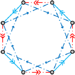
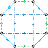
Figure 1: Left: quiver diagram for $Y^{4,4}$. Right: quiver diagram for $Y^{4,0}$.

The charges of the fields under the global symmetries $U(1)_{B}$, $U(1)_{s}$ and $SU(2)_{l}$ and the color-coding of the arrows are indicated below.

(28)

We can refine the index by chemical potentials for the global symmetries,

$${\mathcal{I}}^{\tt L}(t,y,a,b,h) = {\rm Tr}(-1)^{F}\,t^{3(2j_{1}-r)}\,y^{2j_{2}}\,a^{2s}\,b^{2l}\,h^{Q_{B}}\,$$ (29)

$${\mathcal{I}}^{\tt R}(t,y,a,b,h) = {\rm Tr}(-1)^{F}\,t^{3(2j_{2}+r)}\,y^{2j_{1}}\,a^{2s}\,b^{2l}\,h^{Q_{B}}\,.$$ (30)

In practice we can focus on say the left-handed index. The right-handed index of a given theory is obtained from the left-handed index of the same theory by conjugation of the flavor quantum numbers, $a\to 1/a$, $h\to 1/h$.

Given a $Y^{p,q}$ quiver diagram, it is immediate to combine the chiral and vector building blocks (11), (12) and construct the matrix integral that calculates the corresponding index. We illustrate the procedure in the two simplest examples.

$\bullet$ $Y^{1,0}$ ($T^{1,1}$)

The quiver of $T^{1,1}$ is shown in figure 2. The index can be simply read from the quiver diagram,

$$\begin{split}\mathcal{I}_{1,0}=&\prod_{k=1}^{2}\left[\frac{\kappa^{N-1}}{N!}\oint_{\mathbb{T}}\prod^{N-1}_{i=1}\frac{dz^{(k)}_{i}}{2\pi iz^{(k)}_{i}}\frac{1}{\prod_{i\neq j}\Gamma(z^{(k)}_{i}/z^{(k)}_{j})}\right]\\ &\times\prod^{N}_{i,j=1}\Gamma(t^{3r_{U}}b^{\pm}z^{(2)}_{i}/z^{(1)}_{j})\prod^{N}_{i,j=1}\Gamma(t^{3r_{Y}}a^{-1}z^{(1)}_{i}/z^{(2)}_{j})\prod^{N}_{i,j=1}\Gamma(t^{3r_{Z}}a\,z^{(1)}_{i}/z^{(2)}_{j})\end{split}$$ (31)

where the R-charges are

$$r_{U}=r_{Y}=r_{Z}=\frac{1}{2}.$$ (32)

The fact that $Y$ and $Z$ share the same R-charge leads to the symmetry enhancement $U(1)_{s}\to SU(2)_{s}$.

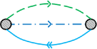
Figure 2: Quiver diagram for $Y^{1,0}$ (the conifold theory $T^{1,1}$). The solid (cyan) arrow represents the $U$ field, the dash-dot (blue) arrow represents the $Y$ field and the dashed (green) arrow represents the $Z$ field.

$\bullet$ $Y^{1,1}$ ($\mathbb{C}^{2}/\mathbb{Z}_{2}\times\mathbb{C}$)

The quiver corresponding to $Y^{1,1}$ is shown in figure 3. This theory is the familiar $\mathbb{Z}_{2}$ orbifold of ${\cal N}=4$ SYM which in fact preserves ${\cal N}=2$ supersymmetry, but we write its ${\cal N}=1$ index for a uniform analysis,

$$\begin{split}\mathcal{I}_{1,1}=&\prod_{k=1}^{2}\left[\frac{\kappa^{N-1}}{N!}\oint_{\mathbb{T}}\prod^{N-1}_{i=1}\frac{dz^{(k)}_{i}}{2\pi iz^{(k)}_{i}}\frac{1}{\prod_{i\neq j}\Gamma(z^{(k)}_{i}/z^{(k)}_{j})}\right]\\ &\times\left[\prod^{N}_{i,j=1}\Gamma(t^{3r_{U}}b^{\pm}z^{(2)}_{i}/z^{(1)}_{j})\prod^{N}_{i,j=1}\Gamma(t^{3r_{V}}b^{\pm}a\,z^{(1)}_{i}/z^{(2)}_{j})\right]\\ &\times\left[\prod^{N}_{i\neq j}\Gamma(t^{3r_{Y}}a^{-1}z^{(1)}_{i}/z^{(1)}_{j})\Gamma(t^{3r_{Y}})^{N-1}\prod^{N}_{i\neq j}\Gamma(t^{3r_{Y}}a^{-1}z^{(2)}_{i}/z^{(2)}_{j})\Gamma(t^{3r_{Y}})^{N-1}\right]\,.\end{split}$$ (33)

Figure 3: Quiver of $Y^{1,1}$ theory. Solid (cyan) arrow represents $U$ field, dash-dot-dot arrow (red) represents $V$ field and dash-dot arrow (blue) represents $Y$ field.

4.1 Toric Duality

A toric Calabi-Yau singularity may have several equivalent quiver representations, related by what has been called “toric duality” [29]. In terms of the gauge theories on D3 branes probing the singularity, two toric-dual quiver diagrams define two UV theories that flow to the same IR superconformal fixed point. Toric duality can in fact be understood in terms of the usual Seiberg duality of super QCD [30, 31, 32, 33, 34, 35, 36]. In particular, the prescription [12] for finding the quiver theory associated $Y^{p,q}$ does not lead to unique answer, rather to a family of quivers related by toric duality. The simplest example occurs for $Y^{4,2}$: the pair of toric-dual quivers associated to $Y^{4,2}$ is shown in figures 4 and 5.

We are now going to check the equality of the indices of two dual theories using an identity between elliptic hypergeometric integrals.

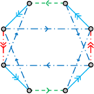
Figure 4: Quiver diagram for $Y^{4,2}$, obtained from $Y^{4,4}$ by using the procedure in [12].

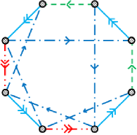
Figure 5: A different quiver diagram for $Y^{4,2}$, related to the diagram above by toric duality.

Consider the $k$-th node of a $Y^{p,q}$ quiver with one incoming $Y$, one incoming $Z$ and an outgoing $U$ doublet (see the first diagram in figure 6). Its contribution to the index (suppressing global symmetry charges) is

$$\begin{split}\mathcal{I}^{k}_{p,q}=&\frac{\kappa^{N-1}}{N!}\oint_{\mathbb{T}}\prod^{N-1}_{i=1}\frac{dz^{(k)}_{i}}{2\pi iz^{(k)}_{i}}\frac{1}{\prod_{i\neq j}\Gamma(z^{(k)}_{i}/z^{(k)}_{j})}\\ &\times\prod_{i,j}\Gamma(t^{3r_{Z}}\frac{z^{k}_{i}}{z^{Z}_{j}})\prod_{i,j}\Gamma(t^{3r_{Y}}\frac{z^{k}_{i}}{z^{Y}_{j}})\prod_{i,j}\Gamma(t^{3r_{U}}\frac{z^{U}_{j}}{z^{k}_{i}})^{2}\prod_{i,j}\Gamma(t^{3r_{V}}\frac{z^{Z}_{i}}{z^{U}_{j}})^{2}.\end{split}$$ (34)

where $z^{U}$, $z^{Y}$ and $z^{Z}$ represents the ”flavor” group of $U$, $Y$ and $Z$. This is precisely the $A_{n}$-type integral defined in [37],

$$\begin{split}\mathcal{I}^{k}_{p,q}=I^{(N-1)}_{A_{N-1}}(Z|t^{3r_{Z}}/z^{Z}_{j},t^{3r_{Y}}/z^{Y}_{j};t^{3r_{U}}z^{U}_{j},t^{3r_{U}}z^{U}_{j};p,q)\prod_{i,j}\Gamma(t^{3r_{V}}\frac{z^{Z}_{i}}{z^{U}_{j}})^{2}\,.\end{split}$$ (35)

This integral obeys the balancing condition

$$\prod_{j=1}^{N}\frac{t^{3r_{Z}}}{z^{Z}_{j}}\frac{t^{3r_{Y}}}{z^{Y}_{j}}t^{3r_{U}}z^{U}_{j}t^{3r_{U}}z^{U}_{j}=(pq)^{N}\,,$$ (36)

thanks to the relation

$$r_{Y}+r_{Z}+2r_{U}=y_{p,q}+x_{p,q}+2[1-\frac{1}{2}(x_{p,q}+y_{p,q})]=2\,.$$ (37)

Then the following identity holds [37]:

$$I^{(m)}_{A_{n}}(Z|t_{i}\ldots,u_{i}\ldots)=\prod_{r,s=1}^{m+n+2}\Gamma(t_{r}u_{s})I^{(n)}_{A_{m}}(Z|\frac{T^{\frac{1}{m+1}}}{t_{i}}\ldots,\frac{U^{\frac{1}{m+1}}}{u_{i}}\ldots).$$ (38)

So we have

$$\begin{split}\mathcal{I}^{k}_{p,q}=&I^{(N-1)}_{A_{N-1}}(Z|t^{3r_{Z}}/z^{Z}_{j},t^{3r_{Y}}/z^{Y}_{j};t^{3r_{U}}z^{U}_{j},t^{3r_{U}}z^{U}_{j};p,q)\prod_{i,j}\Gamma(t^{3r_{V}}\frac{z^{Z}_{i}}{z^{U}_{j}})^{2}\\ =&\prod_{i,j=1}^{N}\Gamma(t^{3(r_{Z}+r_{U})}\frac{z^{U}_{i}}{z^{Z}_{j}})^{2}\prod_{i,j=1}^{N}\Gamma(t^{3(r_{Y}+r_{U})}\frac{z^{U}_{i}}{z^{Y}_{j}})^{2}\\ &\times I^{(N-1)}_{A_{N-1}}(Z|t^{3r_{Y}}z^{Z}_{j},t^{3r_{Z}}z^{Y}_{j};t^{3r_{U}}/z^{U}_{j},t^{3r_{U}}/z^{U}_{j};p,q)\prod_{i,j=1}^{N}\Gamma(t^{3r_{V}}\frac{z^{Z}_{j}}{z^{U}_{i}})^{2}\\ =&\prod_{i,j=1}^{N}\Gamma(t^{3r_{V}}\frac{z^{U}_{i}}{z^{Y}_{j}})^{2}I^{(N-1)}_{A_{N-1}}(Z|t^{3r_{Y}}z^{Z}_{j},t^{3r_{Z}}z^{Y}_{j};t^{3r_{U}}/z^{U}_{j},t^{3r_{U}}/z^{U}_{j};p,q),\end{split}$$ (39)

where we have used $r_{V}=r_{Z}+r_{U}$ and

$$\Gamma(t^{3r_{V}}\frac{z^{Z}_{i}}{z^{U}_{j}})\Gamma(t^{3(r_{Y}+r_{U})}\frac{z^{U}_{j}}{z^{Z}_{i}})=1\,.$$ (40)

      

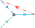
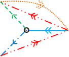
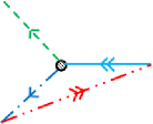
Figure 6: Left: initial quiver. The node represents a $SU(N)$ gauge group. The effective number of flavors is $N_{f}=2N$. Middle: quiver after Seiberg duality. The node represents the Seiberg dual gauge group $SU(2N-N)=SU(N)$. All arrows are reversed and mesons (with appropriate R-charges) are added. Right: the dash-dot-dot (red) and dot (orange) mesons cancel each other out by equ.(4.15). This can be understood physically in terms of integrating out massive degrees of freedom [31].

For example, one can perform this duality on one of the $YZ\bar{U}$ nodes of the $Y^{4,2}$ quiver in figure 4 and obtain the quiver in figure 5. The procedure is illustrated in figure 7.

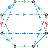
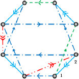
OOOO

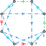
Figure 7: Left: $Y^{4,2}$ quiver in Figure 3. Middle: Seiberg dual on node $1$. Right: the quiver in Figure 4 is obtained by swap node $1$ and $2$ in the middle figure.

This transformation can be represented on a quiver as a local graph transformation of figure 6. It has the interpretation of Seiberg duality on the node. (In fact the same elliptic hypergeometric identity was used in [6] to demonstrate the equality of the index under Seiberg duality.) Iterating this step, we can reach all the toric phases of any $Y^{p,q}$ gauge theory.

5 Large $N$ evaluation of the index

In the large $N$ limit the leading contribution to the index is evaluated using matrix models techniques (see e.g. [23, 1]). Let $\{e^{\alpha_{ai}}\}_{i=1}^{N_{a}}$ denote the $N_{a}$ eigenvalues of $u_{a}$. Then the matrix model integral (9) is,

$${\cal I}(x)=\int\prod_{a,i}[d\alpha_{ai}]\exp\left\{-\sum_{ai\neq bj}V_{b}^{a}(\alpha_{ai}-\alpha_{bj})\right\}\,.$$ (41)

Here, the potential $V$ is the following function

$$V_{b}^{a}(\theta)=\delta_{b}^{a}(\ln 2)+\sum_{n=1}^{\infty}\frac{1}{n}[\delta_{b}^{a}-i_{b}^{a}(x^{n})]\cos n\theta\,,$$ (42)

where, $i_{b}^{a}(x)$ is the total single letter index in the representation $r^{a}\otimes r_{b}$. Writing the density of the eigenvalues $\{e^{\alpha_{ai}}\}$ at the point $\theta$ on the circle as $\rho_{a}(\theta)$, we reduce it to the functional integral problem,

$${\cal I}(x)=\int\prod_{a}[d\rho_{a}]\exp\{-\int d\theta_{1}d\theta_{2}\sum_{a,b}n_{a}n_{b}\rho_{a}(\theta_{1})V_{b}^{a}(\theta_{1}-\theta_{2})\rho_{b}^{\dagger}(\theta_{2})\}\,.$$ (43)

For large $N$, we can evaluate this expression with the saddle point approximation,

$${\cal I}(x) = \prod_{k}\frac{1}{\det(1-i(x^{k}))}\,.$$

For $SU(N)$ gauge groups instead of $U(N)$, the result is modified as follows,

$${\cal I}(x)=\prod_{k}\frac{e^{-\frac{1}{k}\mbox{tr }i(x^{k})}}{\det(1-i(x^{k}))}\,.$$ (44)

Here $i(x)$ is the matrix with entries $i_{b}^{a}(x)$. We will see examples of such matrices below.

The single-trace partition function can be obtained from the full partition function,

$${\cal I}_{s.t.} = \sum_{n=1}^{\infty}\frac{\mu(n)}{n}\log{\cal I}(x^{n})$$ (45)

$$= -\sum_{k=1}^{\infty}\frac{\varphi(k)}{k}\log[\det(1-i(x^{k}))]-\sum_{n=1}^{\infty}\frac{\mu(n)}{n}\sum_{k=1}^{\infty}\frac{\mbox{tr }i(x^{nk})}{k}$$ (46)

$$= -\sum_{k=1}^{\infty}\frac{\varphi(k)}{k}\log[\det(1-i(x^{k}))]-\mbox{tr }i(x)\,.$$ (47)

The second term in the summation would be absent for the $U(N)$ gauge theories. Here $\mu(n)$ is the Möbius function ($\mu(1)\equiv 1,\>\mu(n)\equiv 0$ if $n$ has repeated prime factors and $\mu(n)\equiv(-1)^{k}$ if $n$ is the product of $k$ distinct primes) and $\varphi(n)$ is the Euler Phi function, defined as the number of positive integers less than $n$ that are coprime to $n$. We have used the properties

$$\sum_{d|n}d\mu(\frac{n}{d})=\varphi(n),\qquad\qquad\sum_{d|n}\mu(d)=\delta_{n,1}.$$ (48)

After deriving the general expression for the superconformal index of a quiver gauge theory let us study some concrete examples. Recall the single-letter indices

$$i_{V}(t,y) = \frac{2t^{6}-t^{3}(y+\frac{1}{y})}{(1-t^{3}y)(1-t^{3}y^{-1})}\,,$$ (49)

$$i_{\bar{\chi}(r)}(t,y) = \frac{t^{3r}}{(1-t^{3}y)(1-t^{3}y^{-1})}\,\quad i_{\chi(r)}(t,y)=-\frac{t^{3(2-r)}}{(1-t^{3}y)(1-t^{3}y^{-1})}\,,$$ (50)

where for future convenience we have split the index of the matter multiplet into a chiral and an antichiral contribution. Let us write down explicit expressions for the index in some examples

$\bullet$ $Y^{1,0}\,(T^{1,1})$

For the conifold gauge theory, $U(1)_{s}$ is enhanced to $SU(2)_{s}$ so the global symmetry is $SU(2)_{s}\times SU(2)_{l}$. Assigning the chemical potentials $a$ and $b$, for the two $SU(2)$s, the single letter index matrix $i_{1,0}(t,y)$ is

$$i_{1,0}=\left(\begin{array}[]{cc}i_{V}&(a+\frac{1}{a})(i_{\chi(\frac{1}{2})}+i_{\bar{\chi}(\frac{1}{2})})\\ (b+\frac{1}{b})(i_{\chi(\frac{1}{2})}+i_{\bar{\chi}(\frac{1}{2})})&i_{V}\end{array}\right)\,,$$ (51)

and the single-trace index evaluates to

$${\cal I}_{s.t.} = -\sum_{k=1}^{\infty}\frac{\varphi(k)}{k}\log[(1-i_{V}(x^{k}))^{2}-(a+\frac{1}{a})(b+\frac{1}{b})(i_{\chi(\frac{1}{2})}(x^{k})+i_{\bar{\chi}(\frac{1}{2})}(x^{k}))^{2}]-2i_{V}(x)$$ (52)

$$= \frac{t^{3}ab}{1-t^{3}ab}+\frac{t^{3}\frac{a}{b}}{1-t^{3}\frac{a}{b}}+\frac{t^{3}\frac{b}{a}}{1-t^{3}\frac{b}{a}}+\frac{t^{3}\frac{1}{ab}}{1-t^{3}\frac{1}{ab}}\,.$$

This is the index for the theory where both the overall and the relative $U(1)$ degrees of freedom have been removed. The overall $U(1)$ is completely decoupled, while the relative $U(1)$ has positive beta function and decouples in the IR. The removal of the relative $U(1)$ introduces certain double-trace terms in the superpotential which are important to achieve exact conformality [38]. We have used the following property of Euler Phi function.

$$\sum_{k=1}^{\infty}\frac{\varphi(k)}{k}\log(1-x^{k})=\frac{-x}{1-x}.$$ (53)

We will match the expression (52) to the gravity computation.

$\bullet$ $Y^{1,1}\,(\mathbb{C}^{2}/\mathbb{Z}_{2}\times\mathbb{C})$

The index for this theory was already obtained in [28, 26]. The single letter index matrix $i_{1,1}(t,y)$ is given by

$$i_{1,1}=\left(\begin{array}[]{cc}i_{V}+a^{-1}i_{\chi(\frac{2}{3})}+ai_{\bar{\chi}(\frac{2}{3})}&(b+\frac{1}{b})(ai_{\chi(\frac{2}{3})}+i_{\bar{\chi}(\frac{2}{3})})\\ (b+\frac{1}{b})(i_{\chi(\frac{2}{3})}+a^{-1}i_{\bar{\chi}(\frac{2}{3})})&i_{V}+a^{-1}i_{\chi(\frac{2}{3})}+a\,i_{\bar{\chi}(\frac{2}{3})}\end{array}\right)\,,$$ (54)

and the index evaluates to

$${\cal I}_{s.t.} = -\sum_{k=1}^{\infty}\frac{\varphi(k)}{k}\log[(1-i_{V}(x^{k})-a^{-1}i_{\chi(\frac{2}{3})}(x^{k})-a\,i_{\bar{\chi}(\frac{2}{3})}(x^{k}))^{2}-(b+\frac{1}{b})^{2}\frac{1}{a}(a\,i_{\chi(\frac{2}{3})}(x^{k})+i_{\bar{\chi}(\frac{2}{3})}(x^{k}))^{2}]$$ (55)

$$-2(i_{V}(x)+a^{-1}\,i_{\chi(\frac{2}{3})}(x)+a\,i_{\bar{\chi}(\frac{2}{3})}(x))$$

$$= 2\frac{t^{2}a}{1-t^{2}a}+\frac{t^{4}b^{2}a^{-1}}{1-t^{4}b^{2}a^{-1}}+\frac{t^{4}b^{-2}a^{-1}}{1-t^{4}b^{-2}a^{-1}}-2\frac{a\,t^{2}-a^{-1}\,t^{4}}{(1-t^{3}y)(1-t^{3}y^{-1})}\,.$$

Again, we have subtracted both the overall and relative $U(1)$ degrees of freedom (in this case it is appropriate to subtract ${\cal N}=2$ vector multiplets).

$\bullet$ General $Y^{p,q}$

A simple generalization gives the index for $Y^{p,0}$ ($T^{1,1}/\mathbb{Z}_{p}$) and for $Y^{p,p}$ ($\mathbb{C}^{3}/\mathbb{Z}_{2p}$),

$$Y^{p,p}\;:\qquad \det\left(1-i(t)\right)=\frac{(1-t^{4p})^{2}(1-t^{2p})^{2}}{(1-t^{3}y)^{2p}(1-t^{3}y^{-1})^{2p}}\,,$$ (56)

$$Y^{p,0}\;:\qquad \det\left(1-i(t)\right)=\frac{(1-t^{3p})^{4}}{(1-t^{3}y)^{2p}(1-t^{3}y^{-1})^{2p}}\,.$$

In fact the determinant of the adjacency matrix appears to factorize for general $Y^{p,q}$, to give

$$\det\left(1-i(t)\right)=\frac{\left[1-t^{3p\left(1+{\frac{1}{2}}(x_{p,q}-y_{p,q})\right)}\right]^{2}\,\left[1-t^{3p+\frac{3q}{2}\left(1-{\frac{1}{2}}(x_{p,q}+y_{p,q})\right)}\right]^{2}}{(1-t^{3}y)^{2p}(1-t^{3}y^{-1})^{2p}}\,.$$ (57)

Thus the single-trace partition function is

$${\mathcal{I}}_{p,q}^{s.p.} = 2\left[\frac{t^{\frac{p(3q+2p-\sqrt{4p^{2}-3q^{2}})}{q}}}{1-t^{\frac{p(2p+3q-\sqrt{4p^{2}-3q^{2}})}{q}}}+\frac{t^{\frac{p(3q-2p+\sqrt{4p^{2}-3q^{2}})}{q}}}{1-t^{\frac{p(2p+3q-\sqrt{4p^{2}-3q^{2}})}{q}}}\right]\$$

Again, this is the result with all $U(1)$ factors subtracted. If one introduces a chemical potential $b^{2l}$ for the global $SU(2)_{l}$ and a chemical potential $a^{2s}$ for the global $U(1)_{s}$ of table 28 the index becomes

$${\mathcal{I}}_{p,q}^{s.p.} = \frac{a^{-p}b^{p+q}t^{\frac{p(3q+2p-\sqrt{4p^{2}-3q^{2}})}{q}}}{1-a^{-p}b^{p+q}t^{\frac{p(2p+3q-\sqrt{4p^{2}-3q^{2}})}{q}}}+\frac{a^{-p}b^{-p-q}t^{\frac{p(3q+2p-\sqrt{4p^{2}-3q^{2}})}{q}}}{1-a^{-p}b^{-p-q}t^{\frac{p(2p+3q-\sqrt{4p^{2}-3q^{2}})}{q}}}$$

$$+\frac{a^{p}b^{p-q}t^{\frac{p(3q-2p+\sqrt{4p^{2}-3q^{2}})}{q}}}{1-a^{p}b^{p-q}t^{\frac{p(3q-2p+\sqrt{4p^{2}-3q^{2}})}{q}}}+\frac{a^{p}b^{q-p}t^{\frac{p(3q-2p+\sqrt{4p^{2}-3q^{2}})}{q}}}{1-a^{p}b^{q-p}t^{\frac{p(3q-2p+\sqrt{4p^{2}-3q^{2}})}{q}}}\,.$$

This is the left-handed index. The right-handed index is obtained by letting $a\to 1/a$.

6 $T^{1,1}$ Index from Supergravity

On the dual supergravity side, the index of the conifold theory was computed by Nakayama [14], using the results of [42, 43, 44] for the KK reduction of IIB supergravity on $AdS_{5}\times T^{1,1}$.

Fields	Shortening Cond.	$s$	$l$	Mult.	${\cal I}^{{\tt L}}(t,y)$	$\sum_{\tilde{r}}({\cal I}_{[\tilde{r},j_{2}]_{+}^{{\tt L}}}^{{\tt L}}\times\ldots)$
Graviton	$E=1+\sqrt{H_{0}+4}$	$\frac{r}{2}$	$\frac{r}{2}$	${\cal C}_{r(\frac{1}{2},\frac{1}{2})}$	${\cal I}_{[r+1,\frac{1}{2}]_{-}^{{\tt L}}}^{{\tt L}}$	$-\chi_{\frac{\tilde{r}-1}{2}}(a)\chi_{\frac{\tilde{r}-1}{2}}(b)$
GravitinoI	$E=-\frac{1}{2}+\sqrt{H_{0}^{-}+4}$	$\frac{r-1}{2}$	$\frac{r-1}{2}$	${\cal B}_{r(0,\frac{1}{2})}$	${\cal I}_{[r-2,\frac{1}{2}]_{-}^{{\tt L}}}^{{\tt L}}$	$-\chi_{\frac{\tilde{r}+1}{2}}(a)\chi_{\frac{\tilde{r}+1}{2}}(b)$
		$\frac{r-1}{2}$	$\frac{r+1}{2}$	${\cal C}_{r(0,\frac{1}{2})}$	${\cal I}_{[r,\frac{1}{2}]_{+}^{{\tt L}}}^{{\tt L}}$	$+\chi_{\frac{\tilde{r}-1}{2}}(a)\chi_{\frac{\tilde{r}+1}{2}}(b)$
		$\frac{r+1}{2}$	$\frac{r-1}{2}$	${\cal C}_{r(0,\frac{1}{2})}$	${\cal I}_{[r,\frac{1}{2}]_{+}^{{\tt L}}}^{{\tt L}}$	$+\chi_{\frac{\tilde{r}+1}{2}}(a)\chi_{\frac{\tilde{r}-1}{2}}(b)$
GravitinoIII	$E=-\frac{1}{2}+\sqrt{H_{0}^{+}+4}$	$\frac{r+1}{2}$	$\frac{r+1}{2}$	${\cal C}_{r(\frac{1}{2},0)}$	${\cal I}_{[r+1,0]_{-}^{{\tt L}}}^{{\tt L}}$	$-\chi_{\frac{\tilde{r}}{2}}(a)\chi_{\frac{\tilde{r}}{2}}(b)$
GravitinoIV	$E=\frac{5}{2}+\sqrt{H_{0}^{-}+4}$	$\frac{r-1}{2}$	$\frac{r-1}{2}$	${\cal C}_{r(\frac{1}{2},0)}$	${\cal I}_{[r+1,0]_{-}^{{\tt L}}}^{{\tt L}}$	$-\chi_{\frac{\tilde{r}}{2}-1}(a)\chi_{\frac{\tilde{r}}{2}-1}(b)$
VectorI	$E=-2+\sqrt{H_{0}+4}$	$\frac{r}{2}$	$\frac{r}{2}$	${\cal B}_{r(0,0)}$	${\cal I}_{[r-2,0]_{-}^{{\tt L}}}^{{\tt L}}$	$-\chi_{\frac{\tilde{r}}{2}+1}(a)\chi_{\frac{\tilde{r}}{2}+1}(b)$
		$\frac{r}{2}$	$\frac{r+2}{2}$	${\cal C}_{r(0,0)}$	${\cal I}_{[r,0]_{+}^{{\tt L}}}^{{\tt L}}$	$+\chi_{\frac{\tilde{r}}{2}}(a)\chi_{\frac{\tilde{r}}{2}+1}(b)$
		$\frac{r+2}{2}$	$\frac{r}{2}$	${\cal C}_{r(0,0)}$	${\cal I}_{[r,0]_{+}^{{\tt L}}}^{{\tt L}}$	$+\chi_{\frac{\tilde{r}}{2}+1}(a)\chi_{\frac{\tilde{r}}{2}}(b)$
VectorIV	$E=1+\sqrt{H_{0}^{--}+4}$	$\frac{r-2}{2}$	$\frac{r-2}{2}$	${\cal B}_{r(0,0)}$	${\cal I}_{[r-2,0]_{-}^{{\tt L}}}^{{\tt L}}$	$-\chi_{\frac{\tilde{r}}{2}}(a)\chi_{\frac{\tilde{r}}{2}}(b)$
		$\frac{r-2}{2}$	$\frac{r}{2}$	${\cal C}_{r(0,0)}$	${\cal I}_{[r,0]_{+}^{{\tt L}}}^{{\tt L}}$	$+\chi_{\frac{\tilde{r}}{2}-1}(a)\chi_{\frac{\tilde{r}}{2}}(b)$
		$\frac{r}{2}$	$\frac{r-2}{2}$	${\cal C}_{r(0,0)}$	${\cal I}_{[r,0]_{+}^{{\tt L}}}^{{\tt L}}$	$+\chi_{\frac{\tilde{r}}{2}}(a)\chi_{\frac{\tilde{r}}{2}-1}(b)$

Table 2: Short multiplets appearing in the KK reduction of Type IIB supergravity on $AdS_{5}\times T^{1,1}$. In the last column, we summarize the full index contributions of multiplets by listing the $SU(2)_{s}\times SU(2)_{l}$ characters multiplying ${\cal I}_{[\tilde{r},\frac{1}{2}]_{+}^{{\tt L}}}^{{\tt L}}$ for first four rows and ${\cal I}_{[\tilde{r},0]_{+}^{{\tt L}}}^{{\tt L}}$ for remaining rows. The range of $\tilde{r}$ is specified by the two conditions that $\tilde{r}\geq-1$ and that the $SU(2)_{s}\times SU(2)_{l}$ representation makes sense. The chemical potentials $a$ and $b$ couple to $SU(2)_{s}\times SU(2)_{l}$ flavor charges respectively. Exception: The first row of Gravitino_I starts from $\tilde{r}=0$. The $\tilde{r}=-1$ state of Gravitino_I gives rise to the Dirac multiplet ${\cal D}_{(0,\frac{1}{2})}$ due to additional shortening. It corresponds in the dual field theory to a decoupled $U(1)$ vector multiplet.

Let us briefly review the structure of the calculation. For a general $AdS_{5}\times Y^{p,q}$ background, the KK spectrum organizes itself in three types of multiplets [43, 44]: graviton ($({\frac{1}{2}},{\frac{1}{2}})$), LH-gravitino ($({\frac{1}{2}},0)$), RH-gravitino ($(0,{\frac{1}{2}})$), and vector ($(0,0)$). The details of the specific background manifest themselves in the possible spectrum of the R-charges and their multiplicities. This information can be obtained by solving the spectrum of relevant differential operators, e.g. scalar Laplacian and Dirac operators. For the $Y^{p,q}$ geometries the scalar Laplacian is given by Heun’s differential equation spectrum of which is hard to obtain in closed form, see e.g. [40]. For the $T^{1,1}$ background these data were carefully computed in [42, 43, 44]. A generic multiplet of the KK spectrum does not obey shortening conditions and thus does not contribute to the index. Table 2 summarizes the multiplets which do contribute of the index. The eigenvalue of the scalar laplacian is denoted by $H_{0}(s,l,r)$,

$$H_{0}(s,l,r)=6(s(s+1)+l(l+1)-\frac{r^{2}}{8}).$$ (59)

$H_{0}^{\pm}$ and $H_{0}^{\pm\pm}$ are shorthands for $H_{0}(s,l,r\pm 1)$ and $H_{0}(s,l,r\pm 2)$ respectively. Besides the KK modes of table 2, there are additional Betti multiplets, arising from the non-trivial homology of $T^{1,1}$. Their contribution to the index is found to vanish [14].

The $T^{1,1}$ manifold has $SU(2)_{s}\times SU(2)_{l}$ isometry. We refine the index by adding chemical potentials $a$ and $b$ that couple respectively to $SU(2)_{s}$ and $SU(2)_{l}$. Simply reading off the R-charges and the multiplicities of the different modes, we can write down the index as [14]

$${\cal I}^{{\tt L}} = -\sum_{\tilde{r}\geq 0}{\cal I}_{[\tilde{r},\frac{1}{2}]_{+}^{{\tt L}}}^{{\tt L}}[(ab)^{\tilde{r}+1}+(\frac{a}{b})^{\tilde{r}+1}+(\frac{b}{a})^{\tilde{r}+1}+(\frac{1}{ab})^{\tilde{r}+1}]$$ (60)

$$- \sum_{\tilde{r}\geq-1}{\cal I}_{[\tilde{r},0]_{+}^{{\tt L}}}^{{\tt L}}[(ab)^{\tilde{r}}+(\frac{a}{b})^{\tilde{r}}+(\frac{b}{a})^{\tilde{r}}+(\frac{1}{ab})^{\tilde{r}}+(ab)^{\tilde{r}+2}+(\frac{a}{b})^{\tilde{r}+2}+(\frac{b}{a})^{\tilde{r}+2}+(\frac{1}{ab})^{\tilde{r}+2}]$$

$$+ {\cal I}_{[-1,0]_{+}^{{\tt L}}}^{{\tt L}}\chi_{-\frac{3}{2}}(a)\chi_{-\frac{3}{2}}(b)-{\cal I}_{[0,0]_{+}^{{\tt L}}}^{{\tt L}}[-\chi_{-1}(a)\chi_{-1}(b)+\chi_{-1}(a)\chi_{0}(b)+\chi_{0}(a)\chi_{-1}(b)]$$

The definition of the index building blocks ${\cal I}^{\tt L}_{[\tilde{r},j_{2}]^{\tt L}_{\pm}}$ is given in the appendix, while the symbol $\chi_{j}(x)$ stands for the standard character of the spin-$j$ representation of $SU(2)$,

$$\chi_{j}(x)\equiv\frac{x^{2j+1}-x^{-(2j+1)}}{x-x^{-1}}\,.$$ (61)

After simplification,

$${\cal I}^{{\tt L}}=\frac{t^{3}ab}{1-t^{3}ab}+\frac{t^{3}\frac{a}{b}}{1-t^{3}\frac{a}{b}}+\frac{t^{3}\frac{b}{a}}{1-t^{3}\frac{b}{a}}+\frac{t^{3}\frac{1}{ab}}{1-t^{3}\frac{1}{ab}}\,,$$ (62)

which precisely agrees with the large $N$ index (52) computed from gauge theory using Römelsberger’s prescription.

Appendix A $\mathcal{N}=1$ superconformal shortening conditions and the index

In this appendix we summarize some basic facts about $\mathcal{N}=1$ superconformal representation theory. A generic long multiplet ${\cal A}^{\Delta}_{r(j_{1},j_{2})}$ is generated by the action of $4$ Poincaré supercharges ${\cal Q}_{\alpha}$ and ${\widetilde{\cal Q}}_{\dot{\alpha}}$ on superconformal primary which is by definition is annihilated by all conformal supercharges $\cal S$. In table 3 we have summarized possible shortening and semishortening conditions.

Shortening Conditions				Multiplet
${\cal B}$	${\cal Q}_{\alpha}|r\rangle^{h.w.}=0$	$j_{1}=0$	$\Delta=-\frac{3}{2}r$	${\cal B}_{r(0,j_{2})}$
$\bar{{\cal B}}$	$\bar{{\cal Q}}_{\dot{\alpha}}|r\rangle^{h.w.}=0$	$j_{2}=0$	$\Delta=\frac{3}{2}r$	$\bar{{\cal B}}_{r(j_{1},0)}$
$\hat{{\cal B}}$	${\cal B}\cap\bar{{\cal B}}$	$j_{1},j_{2},r=0$	$\Delta=0$	$\hat{{\cal B}}$
${\cal C}$	$\epsilon^{\alpha\beta}{\cal Q}_{\beta}|r\rangle_{\alpha}^{h.w.}=0$		$\Delta=2+2j_{1}-\frac{3}{2}r$	${\cal C}_{r(j_{1},j_{2})}$
	$({\cal Q})^{2}|r\rangle^{h.w.}=0$ for $j_{1}=0$		$\Delta=2-\frac{3}{2}r$	${\cal C}_{r(0,j_{2})}$
$\bar{{\cal C}}$	$\epsilon^{\dot{\alpha}\dot{\beta}}\bar{{\cal Q}}_{\dot{\beta}}|r\rangle_{\dot{\alpha}}^{h.w.}=0$		$\Delta=2+2j_{2}+\frac{3}{2}r$	$\bar{{\cal C}}_{r(j_{1},j_{2})}$
	$(\bar{{\cal Q}})^{2}|r\rangle^{h.w.}=0$ for $j_{2}=0$		$\Delta=2+\frac{3}{2}r$	$\bar{{\cal C}}_{r(j_{1},0)}$
$\hat{{\cal C}}$	${\cal C}\cap\bar{{\cal C}}$	$\frac{3}{2}r=(j_{1}-j_{2})$	$\Delta=2+j_{1}+j_{2}$	$\hat{{\cal C}}_{(j_{1},j_{2})}$
${\cal D}$	${\cal B}\cap\bar{{\cal C}}$	$j_{1}=0,-\frac{3}{2}r=j_{2}+1$	$\Delta=-\frac{3}{2}r=1+j_{2}$	${\cal D}_{(0,j_{2})}$
$\bar{{\cal D}}$	$\bar{{\cal B}}\cap{\cal C}$	$j_{2}=0,\frac{3}{2}r=j_{1}+1$	$\Delta=\frac{3}{2}r=1+j_{1}$	$\bar{{\cal D}}_{(j_{1},0)}$

Table 3: Possible shortening conditions for the $\mathcal{N}=1$ superconformal algebra.

A generic long multiplet of the ${\cal N}=1$ superconformal algebra $SU(2,2|1)$ is $16(2j_{1}+1,2j_{2}+1)$ dimensional. Tables 4, 5, 6 and 7 illustrate how the ${\cal B}$, ${\cal C}$, $\hat{\cal C}$ and ${\cal D}$-type multiplets fit within a generic long multiplet.

$\begin{array}[]{ccccccccccc}\Delta&&&&&&\boxed{(j_{1},j_{2})}\\ \\ \Delta+\frac{1}{2}&&&&(j_{1}+\frac{1}{2},j_{2})&&&&\boxed{(j_{1},j_{2}+\frac{1}{2})}\\ &&&&(j_{1}-\frac{1}{2},j_{2})&&&&\boxed{(j_{1},j_{2}-\frac{1}{2})}\\ &&&&&&(j_{1}+\frac{1}{2},j_{2}+\frac{1}{2})\\ \Delta+1&&\quad(j_{1},j_{2})&&&&(j_{1}-\frac{1}{2},j_{2}+\frac{1}{2}),(j_{1}+\frac{1}{2},j_{2}-\frac{1}{2})&&&&\qquad\quad\boxed{(j_{1},j_{2})}\\ &&&&&&(j_{1}-\frac{1}{2},j_{2}-\frac{1}{2})\\ \Delta+\frac{3}{2}&&&&(j_{1},j_{2}+\frac{1}{2})&&&&(j_{1}+\frac{1}{2},j_{2})\\ &&&&(j_{1},j_{2}-\frac{1}{2})&&&&(j_{1}-\frac{1}{2},j_{2})\\ \\ \Delta+2&&&&&&(j_{1},j_{2})\\ \\ &&r-2&&r-1&&r&&r+1&&r+2\end{array}$

Table 4: A long multiplet of $\mathcal{N}=1$ superconformal algebra. The $SU(2,2)$ multiplets that are boxed form a short ${\cal B}_{r(0,j_{2})}$ multiplet for $j_{1}=0,\Delta=-\frac{3}{2}r$. The left-handed $\bar{{\cal B}}$ can be obtained by reflecting the table (that is, sending $r\to-r$ and $j_{1}\leftrightarrow j_{2}$). In general, when $j_{1}(j_{2})=0$, the $SU(2,2)$ multiplets $(j_{1}-\frac{1}{2},any)((any,j_{2}-\frac{1}{2}))$ are set to zero, resulting in further shortening.

$\begin{array}[]{ccccccccccc}\Delta&&&&&&\boxed{(j_{1},j_{2})}\\ \\ \Delta+\frac{1}{2}&&&&\boxed{(j_{1}+\frac{1}{2},j_{2})}&&&&\boxed{(j_{1},j_{2}+\frac{1}{2})}\\ &&&&(j_{1}-\frac{1}{2},j_{2})&&&&\boxed{(j_{1},j_{2}-\frac{1}{2})}\\ &&&&&&\boxed{(j_{1}+\frac{1}{2},j_{2}+\frac{1}{2})}\\ \Delta+1&&\quad(j_{1},j_{2})&&&&(j_{1}-\frac{1}{2},j_{2}+\frac{1}{2})\boxed{(j_{1}+\frac{1}{2},j_{2}-\frac{1}{2})}&&&&\qquad\quad\boxed{(j_{1},j_{2})}\\ &&&&&&(j_{1}-\frac{1}{2},j_{2}-\frac{1}{2})\\ \Delta+\frac{3}{2}&&&&(j_{1},j_{2}+\frac{1}{2})&&&&\boxed{(j_{1}+\frac{1}{2},j_{2})}\\ &&&&(j_{1},j_{2}-\frac{1}{2})&&&&(j_{1}-\frac{1}{2},j_{2})\\ \\ \Delta+2&&&&&&(j_{1},j_{2})\\ \\ &&r-2&&r-1&&r&&r+1&&r+2\end{array}$

Table 5: A long multiplet of $\mathcal{N}=1$ superconformal algebra. The $SU(2,2)$ multiplets that are boxed form a semi-short ${\cal C}_{r(j_{1},j_{2})}$ multiplet for $\Delta=2+2j_{1}-\frac{3}{2}r$. The left-handed $\bar{{\cal C}}$ can be obtained by reflecting the table (that is, sending $r\to-r$ and $j_{1}\leftrightarrow j_{2}$). In general, when $j_{1}(j_{2})=0$, the $SU(2,2)$ multiplets $(j_{1}-\frac{1}{2},any)((any,j_{2}-\frac{1}{2}))$ are set to zero, resulting in further shortening.

$\begin{array}[]{ccccccccccc}\Delta&&&&&&\boxed{(j_{1},j_{2})}\\ \\ \Delta+\frac{1}{2}&&&&\boxed{(j_{1}+\frac{1}{2},j_{2})}&&&&\boxed{(j_{1},j_{2}+\frac{1}{2})}\\ &&&&(j_{1}-\frac{1}{2},j_{2})&&&&(j_{1},j_{2}-\frac{1}{2})\\ &&&&&&\boxed{(j_{1}+\frac{1}{2},j_{2}+\frac{1}{2})}\\ \Delta+1&&(j_{1},j_{2})&&&&(j_{1}-\frac{1}{2},j_{2}+\frac{1}{2})\quad(j_{1}+\frac{1}{2},j_{2}-\frac{1}{2})&&&&\qquad\quad(j_{1},j_{2})\\ &&&&&&\boxed{-(j_{1}-\frac{1}{2},j_{2}-\frac{1}{2})}\\ \Delta+\frac{3}{2}&&&&(j_{1},j_{2}+\frac{1}{2})&&&&(j_{1}+\frac{1}{2},j_{2})\\ &&&&\boxed{-(j_{1},j_{2}-\frac{1}{2})}&&&&\boxed{-(j_{1}-\frac{1}{2},j_{2})}\\ \\ \Delta+2&&&&&&\boxed{-(j_{1},j_{2})}\\ \\ &&r-2&&r-1&&r&&r+1&&r+2\end{array}$

Table 6: Multiplet structure of $\hat{{\cal C}}_{(j_{1},j_{2})}$. The shortening conditions are $\Delta=2+j_{1}+j_{2}$ and $\frac{3}{2}r=(j_{1}-j_{2})$.

$\begin{array}[]{ccccccccccc}\Delta&&&&&&\boxed{(j_{1},j_{2})}\\ \\ \Delta+\frac{1}{2}&&&&(j_{1}+\frac{1}{2},j_{2})&&&&\boxed{(j_{1},j_{2}+\frac{1}{2})}\\ &&&&(j_{1}-\frac{1}{2},j_{2})&&&&(j_{1},j_{2}-\frac{1}{2})\\ &&&&&&(j_{1}+\frac{1}{2},j_{2}+\frac{1}{2})\\ \Delta+1&&(j_{1},j_{2})&&&&(j_{1}-\frac{1}{2},j_{2}+\frac{1}{2}),\boxed{-(j_{1}+\frac{1}{2},j_{2}-\frac{1}{2})}&&&&\qquad\quad(j_{1},j_{2})\\ &&&&&&(j_{1}-\frac{1}{2},j_{2}-\frac{1}{2})\\ \Delta+\frac{3}{2}&&&&(j_{1},j_{2}+\frac{1}{2})&&&&\boxed{-(j_{1}+\frac{1}{2},j_{2})}\\ &&&&(j_{1},j_{2}-\frac{1}{2})&&&&(j_{1}-\frac{1}{2},j_{2})\\ \\ \Delta+2&&&&&&(j_{1},j_{2}),\boxed{+(j_{1},j_{2}-1)}\\ \\ \\ \Delta+\frac{5}{2}&&&&&&&&\boxed{+(j_{1},j_{2}-\frac{1}{2})}\\ \\ &&r-2&&r-1&&r&&r+1&&r+2\end{array}$

Table 7: Multiplet structure of ${\cal D}_{(0,j_{2})}$. The shortening conditions are $\Delta=1+j_{2}=-\frac{3}{2}r$ and $j_{1}=0$. The multiplet $\bar{{\cal D}}_{(j_{1},0)}$ could be obtained by $j_{1}\leftrightarrow j_{2},r\leftrightarrow-r$ or by simply reflecting the table. The shortening conditions in that case are $\Delta=1+j_{1}=\frac{3}{2}r$ and $j_{2}=0$.

At the unitarity threshold, a long multiplet can decompose into (semi)short multiplets. The splitting rules are:

$${\cal A}_{r(j_{1},j_{2})}^{2+2j_{1}-\frac{3}{2}r} \simeq {\cal C}_{r(j_{1},j_{2})}\oplus{\cal C}_{r-1(j_{1}-\frac{1}{2},j_{2})}$$

$${\cal A}_{r(j_{1},j_{2})}^{2+2j_{2}+\frac{3}{2}r} \simeq \bar{{\cal C}}_{r(j_{1},j_{2})}\oplus\bar{{\cal C}}_{r+1(j_{1},j_{2}-\frac{1}{2})}$$

$${\cal A}_{\frac{2}{3}(j_{1}-j_{2})(j_{1},j_{2})}^{2+j_{1}+j_{2}} \simeq \hat{{\cal C}}_{(j_{1},j_{2})}\oplus{\cal C}_{\frac{2}{3}(j_{1}-j_{2})-1,(j_{1}-\frac{1}{2},j_{2})}\oplus\bar{{\cal C}}_{\frac{2}{3}(j_{1}-j_{2})+1,(j_{1},j_{2}-\frac{1}{2})}$$

We are using a notation where the ${\cal B}$ and $\bar{{\cal B}}$ type multiplets are formally identified with special cases of ${\cal C}$ and $\bar{{\cal C}}$ multiplets, as follows

$${\cal C}_{r(-\frac{1}{2},j_{2})}\simeq{\cal B}_{r-1(0,j_{2})}\qquad\bar{{\cal C}}_{r(j_{1},-\frac{1}{2})}\simeq\bar{{\cal B}}_{r+1(j_{1},0)}\,.$$ (63)

We define the ${\tt L}$eft (${\tt R}$ight) equivalence class of the multiplet ${\cal C}_{r(j_{1},j_{2})}(\bar{{\cal C}}_{r(j_{1},j_{2})})$ as the class of multiplets with the same ${\tt L}$eft (${\tt R}$ight) index. From the splitting rules, we see that the classes can be labeled as $[-r+2j_{1},j_{2}]_{(-)^{2j_{1}}}^{{\tt L}}$ $([r+2j_{2},j_{1}]_{(-)^{2j_{2}}}^{{\tt R}})$. Moreover, ${\cal I}_{[-r+2j_{1},j_{2}]_{-}^{{\tt L}}}^{{\tt L}}=-{\cal I}_{[-r+2j_{1},j_{2}]_{+}^{{\tt L}}}^{{\tt L}}$ and ${\cal I}_{[r+2j_{2},j_{1}]_{-}^{{\tt R}}}^{{\tt R}}=-{\cal I}_{[r+2j_{2},j_{1}]_{+}^{{\tt R}}}^{{\tt R}}$. The expressions for the indices of the equivalent classes are

$${\cal I}_{[\tilde{r},j_{2}]_{\pm}^{{\tt L}}}^{{\tt L}} = \pm(-)^{2j_{2}+1}\frac{t^{3(\tilde{r}+2)}\chi_{j_{2}}(y)}{(1-t^{3}y)(1-t^{3}y^{-1})}$$

$${\cal I}_{[\bar{\tilde{r}},j_{1}]_{\pm}^{{\tt R}}}^{{\tt R}} = \pm(-)^{2j_{1}+1}\frac{t^{3(\bar{\tilde{r}}+2)}\chi_{j_{1}}(y)}{(1-t^{3}y)(1-t^{3}y^{-1})}\,$$

$${\cal I}^{R}[\tilde{r},j_{2}]_{\pm}^{{\tt L}} = 0$$

$${\cal I}^{{\tt L}}[\bar{\tilde{r}},j_{1}]_{\pm}^{{\tt R}} = 0\,.$$

The situation is slightly more involved for the $\hat{{\cal C}}$ and ${\cal D}$ type multiplets. Unlike the ${\cal B},{\cal C}$ type multiplets, they contribute both to ${\cal I}^{{\tt L}}$ as well as ${\cal I}^{{\tt R}}$. The indices [6] for the different types of multiplets are collected in table 8.

Multiplet	${\cal I}^{{\tt L}}$	${\cal I}^{{\tt R}}$
${\cal A}_{r(j_{1},j_{2})}^{\Delta}$	$0$	$0$
${\cal C}_{r(j_{1},j_{2})}$	${\cal I}_{[-r+2j_{1},j_{2}]_{(-)^{2j_{1}}}^{{\tt L}}}^{{\tt L}}$	$0$
$\bar{{\cal C}}_{r(j_{1},j_{2})}$	$0$	${\cal I}_{[r+2j_{2},j_{1}]_{(-)^{2j_{2}}}^{{\tt R}}}^{{\tt R}}$
$\hat{{\cal C}}_{(j_{1},j_{2})}$	${\cal I}_{[\frac{2}{3}j_{2}+\frac{4}{3}j_{1},j_{2}]_{(-)^{2j_{1}}}^{{\tt L}}}^{{\tt L}}$	${\cal I}_{[\frac{2}{3}j_{1}+\frac{4}{3}j_{2},j_{1}]_{(-)^{2j_{2}}}^{{\tt R}}}^{{\tt R}}$
${\cal D}_{(0,j_{2})}$	${\cal I}_{[\frac{2}{3}j_{2}-\frac{4}{3},j_{2}]_{-}^{{\tt L}}}^{{\tt L}}+{\cal I}_{[\frac{2}{3}j_{2}-\frac{1}{3},j_{2}-\frac{1}{2}]_{-}^{{\tt L}}}^{{\tt L}}$	${\cal I}_{[\frac{4}{3}j_{2}-\frac{2}{3},0]_{+}^{{\tt R}}}^{{\tt R}}$
$\bar{{\cal D}}_{(j_{1},0)}$	${\cal I}_{[\frac{4}{3}j_{1}-\frac{2}{3},0]_{+}^{{\tt L}}}^{{\tt L}}$	${\cal I}_{[\frac{2}{3}j_{1}-\frac{4}{3},j_{1}]_{-}^{{\tt R}}}^{{\tt R}}+{\cal I}_{[\frac{2}{3}j_{1}-\frac{1}{3},j_{1}-\frac{1}{2}]_{-}^{{\tt R}}}^{{\tt R}}$

Table 8: Indices ${\cal I}^{{\tt L}}$ and ${\cal I}^{{\tt R}}$ of the various short and semi-short multiplets.

References

- [1] J. Kinney, J. M. Maldacena, S. Minwalla, and S. Raju, An index for 4 dimensional super conformal theories, Commun. Math. Phys. 275 (2007) 209–254, [hep-th/0510251].
- [2] A. Gadde, E. Pomoni, L. Rastelli, and S. S. Razamat, S-duality and 2d Topological QFT, JHEP 03 (2010) 032, [0910.2225].
- [3] A. Gadde, L. Rastelli, S. S. Razamat, and W. Yan, The Superconformal Index of the SCFT, JHEP 08 (2010) 107, [1003.4244].
- [4] C. Romelsberger, Counting chiral primaries in N = 1, d=4 superconformal field theories, Nucl. Phys. B747 (2006) 329–353, [hep-th/0510060].
- [5] C. Romelsberger, Calculating the Superconformal Index and Seiberg Duality, 0707.3702.
- [6] F. A. Dolan and H. Osborn, Applications of the Superconformal Index for Protected Operators and q-Hypergeometric Identities to N=1 Dual Theories, Nucl. Phys. B818 (2009) 137–178, [arXiv:0801.4947].
- [7] V. P. Spiridonov and G. S. Vartanov, Superconformal indices for theories with multiple duals, Nucl. Phys. B824 (2010) 192–216, [0811.1909].
- [8] V. P. Spiridonov and G. S. Vartanov, Elliptic hypergeometry of supersymmetric dualities, 0910.5944.
- [9] V. Spiridonov and G. Vartanov, Supersymmetric dualities beyond the conformal window, Phys.Rev.Lett. 105 (2010) 061603, [1003.6109].
- [10] G. Vartanov, On the ISS model of dynamical SUSY breaking, 1009.2153.
- [11] I. R. Klebanov and E. Witten, Superconformal field theory on three-branes at a Calabi-Yau singularity, Nucl.Phys. B536 (1998) 199–218, [hep-th/9807080].
- [12] S. Benvenuti, S. Franco, A. Hanany, D. Martelli, and J. Sparks, An infinite family of superconformal quiver gauge theories with Sasaki-Einstein duals, JHEP 06 (2005) 064, [hep-th/0411264].
- [13] M. Cvetic, H. Lu, D. N. Page, and C. Pope, New Einstein-Sasaki spaces in five and higher dimensions, Phys.Rev.Lett. 95 (2005) 071101, [hep-th/0504225].
- [14] Y. Nakayama, Index for supergravity on AdS(5) x T**1,1 and conifold gauge theory, Nucl.Phys. B755 (2006) 295–312, [hep-th/0602284].
- [15] K. A. Intriligator and B. Wecht, The Exact superconformal R symmetry maximizes a, Nucl.Phys. B667 (2003) 183–200, [hep-th/0304128].
- [16] O. Aharony, J. Marsano, S. Minwalla, K. Papadodimas, and M. Van Raamsdonk, A first order deconfinement transition in large N Yang- Mills theory on a small 3-sphere, Phys. Rev. D71 (2005) 125018, [hep-th/0502149].
- [17] O. Aharony, J. Marsano, and M. Van Raamsdonk, Two loop partition function for large N pure Yang-Mills theory on a small S**3, Phys. Rev. D74 (2006) 105012, [hep-th/0608156].
- [18] M. Mussel and R. Yacoby, The 2-loop partition function of large N gauge theories with adjoint matter on , JHEP 12 (2009) 005, [0909.0407].
- [19] G. Ishiki, Y. Takayama, and A. Tsuchiya, N = 4 SYM on R x S**3 and theories with 16 supercharges, JHEP 10 (2006) 007, [hep-th/0605163].
- [20] E. Witten, Constraints on Supersymmetry Breaking, Nucl. Phys. B202 (1982) 253.
- [21] B. Feng, A. Hanany, and Y.-H. He, Counting Gauge Invariants: the Plethystic Program, JHEP 03 (2007) 090, [hep-th/0701063].
- [22] S. Benvenuti, B. Feng, A. Hanany, and Y.-H. He, Counting BPS operators in gauge theories: Quivers, syzygies and plethystics, JHEP 11 (2007) 050, [hep-th/0608050].
- [23] O. Aharony, J. Marsano, S. Minwalla, K. Papadodimas, and M. Van Raamsdonk, The Hagedorn / deconfinement phase transition in weakly coupled large N gauge theories, Adv. Theor. Math. Phys. 8 (2004) 603–696, [hep-th/0310285].
- [24] F. Benini, Y. Tachikawa, and B. Wecht, Sicilian gauge theories and N=1 dualities, arXiv:0909.1327.
- [25] Y. Tachikawa and B. Wecht, Explanation of the Central Charge Ratio 27/32 in Four- Dimensional Renormalization Group Flows between Superconformal Theories, Phys. Rev. Lett. 103 (2009) 061601, [0906.0965].
- [26] A. Gadde, E. Pomoni, and L. Rastelli, The Veneziano Limit of N=2 Superconformal QCD: Towards the String Dual of SYM with , 0912.4918.
- [27] M. Yamazaki, Brane Tilings and Their Applications, Fortsch. Phys. 56 (2008) 555–686, [0803.4474].
- [28] Y. Nakayama, Index for orbifold quiver gauge theories, Phys. Lett. B636 (2006) 132–136, [hep-th/0512280].
- [29] B. Feng, A. Hanany, and Y.-H. He, D-brane gauge theories from toric singularities and toric duality, Nucl. Phys. B595 (2001) 165–200, [hep-th/0003085].
- [30] C. E. Beasley and M. R. Plesser, Toric duality is Seiberg duality, JHEP 12 (2001) 001, [hep-th/0109053].
- [31] B. Feng, A. Hanany, Y.-H. He, and A. M. Uranga, Toric duality as Seiberg duality and brane diamonds, JHEP 12 (2001) 035, [hep-th/0109063].
- [32] H. Ooguri and C. Vafa, Geometry of N = 1 dualities in four dimensions, Nucl. Phys. B500 (1997) 62–74, [hep-th/9702180].
- [33] F. Cachazo, B. Fiol, K. A. Intriligator, S. Katz, and C. Vafa, A geometric unification of dualities, Nucl. Phys. B628 (2002) 3–78, [hep-th/0110028].
- [34] B. Feng, A. Hanany, and Y.-H. He, Phase structure of D-brane gauge theories and toric duality, JHEP 08 (2001) 040, [hep-th/0104259].
- [35] B. Feng, S. Franco, A. Hanany, and Y.-H. He, Symmetries of toric duality, JHEP 12 (2002) 076, [hep-th/0205144].
- [36] S. Franco, A. Hanany, Y.-H. He, and P. Kazakopoulos, Duality walls, duality trees and fractional branes, hep-th/0306092.
- [37] E. M. Rains, Transformations of Elliptic Hypergeometric Integrals , math/0309252.
- [38] A. Dymarsky, I. Klebanov, and R. Roiban, Perturbative gauge theory and closed string tachyons, JHEP 0511 (2005) 038, [hep-th/0509132].
- [39] S. Benvenuti and M. Kruczenski, Semiclassical strings in Sasaki-Einstein manifolds and long operators in N = 1 gauge theories, JHEP 10 (2006) 051, [hep-th/0505046].
- [40] H. Kihara, M. Sakaguchi, and Y. Yasui, Scalar Laplacian on Sasaki-Einstein manifolds Y(p,q), Phys. Lett. B621 (2005) 288–294, [hep-th/0505259].
- [41] T. Oota and Y. Yasui, Toric Sasaki-Einstein manifolds and Heun equations, Nucl. Phys. B742 (2006) 275–294, [hep-th/0512124].
- [42] S. S. Gubser, Einstein manifolds and conformal field theories, Phys. Rev. D59 (1999) 025006, [hep-th/9807164].
- [43] A. Ceresole, G. Dall’Agata, R. D’Auria, and S. Ferrara, Spectrum of type IIB supergravity on AdS(5) x T(11): Predictions on N = 1 SCFT’s, Phys. Rev. D61 (2000) 066001, [hep-th/9905226].
- [44] A. Ceresole, G. Dall’Agata, and R. D’Auria, KK spectroscopy of type IIB supergravity on AdS(5) x T(11), JHEP 11 (1999) 009, [hep-th/9907216].