Abstract

A signal of two leptons and missing energy is challenging to analyze at the Large Hadron Collider (LHC) since it offers only few kinematical handles. This signature generally arises from pair production of heavy charged particles which each decay into a lepton and a weakly interacting stable particle. Here this class of processes is analyzed with minimal model assumptions by considering all possible combinations of spin 0, $\frac{1}{2}$ or 1, and of weak iso-singlets, -doublets or -triplets for the new particles. Adding to existing work on mass and spin measurements, two new variables for spin determination and an asymmetry for the determination of the couplings of the new particles are introduced. It is shown that these observables allow one to independently determine the spin and the couplings of the new particles, except for a few cases that turn out to be indistinguishable at the LHC. These findings are corroborated by results of an alternative analysis strategy based on an automated likelihood test.

1 Introduction

Many models beyond the standard model (SM) include stable weekly interacting massive particles which could be constituents of dark matter. Since the stability of these particles is generally related to some symmetry, they can be produced only in pairs at colliders, leading to challenging signatures with at least two invisible objects. At hadron accelerators like the Large Hadron Collider (LHC) such a signal is not sufficiently kinematically constrained to enable the use of direct reconstruction techniques, and thus it is very difficult to uniquely determine the properties of the produced particles.

One of the most challenging cases are processes with a low-multiplicity final state of only two visible objects, which is focus of this article. In particular we will consider the production of a pair of oppositely charged heavy new particles $Y^{\pm}$ at the LHC, which each decay into a SM lepton and an invisible neutral massive particle $X^{0}$:

$$pp\to Y^{+}Y^{-}\to\ell^{+}\ell^{-}X^{0}\bar{X}^{0},\qquad(\ell=e,\mu).$$ (1)

Several methods for determining the $Y$ and $X$ masses in processes of this type have been proposed in the literature [1, 2, 3, 4]. Furthermore, a number of authors have studied how to extract spin information from angular distributions [5, 6, 7] and the total production rate [8]. To the best knowledge of the authors, however, the problem of determining the couplings of the new particles, which are related to their gauge group representations, has not yet been considered.

The goal of this article is to analyze the process (1) in a more model-independent approach by considering all possible assignments for spins (up to spin one) and SU(2) representations (up to triplets) for the particles $X$ and $Y$. To discriminate between these template model combinations, we discuss several variables for the measurement of masses, spins, and interactions of the new particles, including two new spin-sensitive observables and one new observable for the coupling determination. To minimize model dependence, the total cross section is not considered in this set of variables.

Besides using dedicated observables, we also study an alternative analysis strategy based on an automated likelihood test. This method matches the observed lepton momenta in a sample of events to the corresponding momenta of a theoretically calculated matrix element in a given model and calculates a likelihood from that [9, 10]. Note that the two approaches based on specific observables and on the automated likelihood test are complementary. The latter often reaches a higher statistical significance due to the fact that no information is lost by projecting onto some variables, but it does not permit a straightforward separation between individual particle properties, such as spin and couplings.

After characterizing all relevant spin and coupling representations in section 2 and identifying 11 independent model combinations, we present observables for the measurement of particle properties in section 3 and demonstrate their usefulness in a Monte-Carlo study. Section 4 is devoted to the analysis of the same set of template models with the likelihood test method. Finally, our conclusions are given in section 5.

2 Setup

The class of processes under consideration each involve Drell-Yan–type production of a pair of charged heavy particles $Y^{\pm}$, which each subsequently decay into a lepton $\ell^{\pm}$ ($\ell=e,\mu$) and a neutral heavy particle $X^{0}$, see Fig. 1. It is assumed that the $Y^{\pm}$ and $X^{0}$ are charged under some discrete symmetry, such that they can be produced only in pairs and the lighter new particle ($X^{0}$) is stable and escapes from the detector without leaving a signal. The observable signature thus consists of two same-flavor opposite-sign leptons and missing momentum: $\ell^{+}\ell^{-}+\makebox[1.29167pt][l]{$E$}/\,$. For this process it is insubstantial whether $X^{0}$ is self-conjugate or not.

Figure 1: Basic diagram topology for the new physics processes under consideration. Thick lines indicate new particles, while thin lines denote SM particles.

For the purpose of this work it is assumed that no other new heavy particles play a role in the s- or t-channel of the $Y^{+}Y^{-}$ production process [note, however, that if $Y$ is a vector boson this assumption is not valid, as will be explained below]. In fact, LHC data itself will be able to set a strong lower bound on such particles: searches for di-jet resonances could rule out s-channel resonances that couple to light quarks up to several TeV, and any new particles in the t-channel need to be colored and thus could be produced directly with large cross sections unless their masses are larger than 2–3 TeV [11]. Therefore, if the LHC does not see any such signals, one can safely neglect the presence of extra particles in the s- and t-channel for the production of $Y^{+}Y^{-}$ pairs with mass of a few hundred GeV.

	$Y$	$X$	$\ell$	$ZYY$	$XY\ell$	sample model and decay
	$s$, $I_{\rm SU(2)}$	$s$, $I_{\rm SU(2)}$	$I_{\rm SU(2)}$	coupling	coupling	$Y^{-}\to\ell^{-}X$
1	0, 1	$\frac{1}{2}$, 1	1	$Z^{\mu}Y^{*}\!\overleftrightarrow{\partial}_{\!\!\!\mu}Y$	$\overline{X}\frac{1+\gamma_{5}}{2}\ell\,Y^{*}$	MSSM	$\tilde{\ell}_{\rm R}^{-}\to\ell^{-}\tilde{B}^{0}$
1a	0, 1	$\frac{1}{2}$, 2	2	$Z^{\mu}Y^{*}\!\overleftrightarrow{\partial}_{\!\!\!\mu}Y$	$\overline{X}\frac{1-\gamma_{5}}{2}\ell\,Y^{*}$	MSSM	$\tilde{\ell}_{\rm R}^{-}\to\ell^{-}\tilde{H}^{0}$
2	0, 2	$\frac{1}{2}$, 1	2	$Z^{\mu}Y^{*}\!\overleftrightarrow{\partial}_{\!\!\!\mu}Y$	$\overline{X}\frac{1-\gamma_{5}}{2}\ell\,Y^{*}$	MSSM	$\tilde{\ell}_{\rm L}^{-}\to\ell^{-}\tilde{B}^{0}$
2a	0, 2	$\frac{1}{2}$, 2	1	$Z^{\mu}Y^{*}\!\overleftrightarrow{\partial}_{\!\!\!\mu}Y$	$\overline{X}\frac{1+\gamma_{5}}{2}\ell\,Y^{*}$	MSSM	$\tilde{\ell}_{\rm L}^{-}\to\ell^{-}\tilde{H}^{0}$
2b	0, 2	$\frac{1}{2}$, 3	2	$Z^{\mu}Y^{*}\!\overleftrightarrow{\partial}_{\!\!\!\mu}Y$	$\overline{X}\frac{1-\gamma_{5}}{2}\ell\,Y^{*}$	MSSM	$\tilde{\ell}_{\rm L}^{-}\to\ell^{-}\tilde{W}^{0}$
3	0, 3	$\frac{1}{2}$, 2	2	$Z^{\mu}Y^{*}\!\overleftrightarrow{\partial}_{\!\!\!\mu}Y$	$\overline{X}\frac{1-\gamma_{5}}{2}\ell\,Y^{*}$	UED6	$W_{H,(1)}^{-}\to\ell^{-}\nu_{(1)}$
4	$\frac{1}{2}$, 1	0, 1	1	$\overline{Y}\makebox[1.72218pt][l]{$Z$}/\,Y$	$\overline{Y}\frac{1+\gamma_{5}}{2}\ell\,X$	UED6	$\ell_{S,(1)}^{-}\to\ell^{-}B_{H,(1)}^{0}$
5	$\frac{1}{2}$, 1	0, 2	2	$\overline{Y}\makebox[1.72218pt][l]{$Z$}/\,Y$	$\overline{Y}\frac{1-\gamma_{5}}{2}\ell\,X$	UED	$\ell_{S,(1)}^{-}\to\ell^{-}H_{(1)}^{0}$
6	$\frac{1}{2}$, 1	1, 1	1	$\overline{Y}\makebox[1.72218pt][l]{$Z$}/\,Y$	$\overline{Y}\makebox[1.72218pt][l]{$X$}/\,\frac{1+\gamma_{5}}{2}\ell$	UED	$\ell_{S,(1)}^{-}\to\ell^{-}B_{\mu,(1)}^{0}$
7	$\frac{1}{2}$, 2	0, 1	2	$\overline{Y}\makebox[1.72218pt][l]{$Z$}/\,Y$	$\overline{Y}\frac{1-\gamma_{5}}{2}\ell\,X$	UED6	$\ell_{D,(1)}^{-}\to\ell^{-}B_{H,(1)}^{0}$
7a	$\frac{1}{2}$, 2	0, 3	2	$\overline{Y}\makebox[1.72218pt][l]{$Z$}/\,Y$	$\overline{Y}\frac{1-\gamma_{5}}{2}\ell\,X$	UED6	$\ell_{D,(1)}^{-}\to\ell^{-}W_{H,(1)}^{0}$
8	$\frac{1}{2}$, 2	0, 2	1	$\overline{Y}\makebox[1.72218pt][l]{$Z$}/\,Y$	$\overline{Y}\frac{1+\gamma_{5}}{2}\ell\,X$	MSSM	$\tilde{H}^{-}\to\ell^{-}\tilde{\nu}$
9	$\frac{1}{2}$, 2	1, 1	2	$\overline{Y}\makebox[1.72218pt][l]{$Z$}/\,Y$	$\overline{Y}\makebox[1.72218pt][l]{$X$}/\,\frac{1-\gamma_{5}}{2}\ell$	UED	$\ell_{D,(1)}^{-}\to\ell^{-}B_{\mu,(1)}^{0}$
9a	$\frac{1}{2}$, 2	1, 3	2	$\overline{Y}\makebox[1.72218pt][l]{$Z$}/\,Y$	$\overline{Y}\makebox[1.72218pt][l]{$X$}/\,\frac{1-\gamma_{5}}{2}\ell$	UED	$\ell_{D,(1)}^{-}\to\ell^{-}W_{\mu,(1)}^{0}$
10	$\frac{1}{2}$, 3	0, 2	2	$\overline{Y}\makebox[1.72218pt][l]{$Z$}/\,Y$	$\overline{Y}\frac{1-\gamma_{5}}{2}\ell\,X$	MSSM	$\tilde{W}^{-}\to\ell^{-}\tilde{\nu}$
11	1, 3	$\frac{1}{2}$, 2	2	$S[Z,Y,Y^{*}]$	$\overline{X}\makebox[0.86108pt][l]{$Y$}/\,^{*}\frac{1-\gamma_{5}}{2}\ell$	UED	$W_{\mu,(1)}^{-}\to\ell^{-}\nu_{(1)}$

$A\!\overleftrightarrow{\partial}_{\!\!\!\mu}B\equiv A(\partial_{\mu}B)-(\partial_{\mu}A)B,$

$S[Z,Y,Y^{*}]\equiv Z_{\mu}\,Y^{*}_{\nu}\!\overleftrightarrow{\partial}^{\!\!\!\mu}Y^{\nu}+Y_{\mu}\,Z_{\nu}\!\overleftrightarrow{\partial}^{\!\!\!\mu}Y^{*\nu}+Y^{*}_{\mu}\,Y_{\nu}\!\overleftrightarrow{\partial}^{\!\!\!\mu}Z^{\nu}$

Table 1: List of different assignments of spin $s$ and SU(2) representations for the charged field $Y$ and the neutral field $X$. We define $Y^{-}/Y^{+}$ to be the particle/anti-particle. Also shown are the structure of the couplings to the $Z$ boson and to SM leptons, as well as examples for realizations of these assignments in known models. MSSM refers to the Minimal Supersymmetric Standard Model, UED to (at least) one universal extra dimension, and UED to (at least) two universal extra dimensions. $\tilde{\ell}_{\rm R}^{-}$, $\tilde{\ell}_{\rm L}^{-}$, $\tilde{\nu}$, $\tilde{B}^{0}$, $\tilde{W}^{0,\pm}$, and $\tilde{H}$ denote the superpartners of the right-handed charged lepton, left-handed charged lepton, neutrino, U(1) gauge field, SU(2) gauge fields, and Higgs boson, respectively. $\ell^{-}_{S,(1)}$, $\ell^{-}_{D,(1)}$, $\nu_{(1)}$, $\tilde{B}^{0}_{\mu,(1)}$, $\tilde{W}^{0,\pm}_{\mu,(1)}$, and $\tilde{H}_{(1)}$, respectively, are the first-level KK-excitations of these fields. $B_{H,(1)}^{0}$ and $W_{H,(1)}^{0}$ are scalars stemming from one of the extra components of the higher-dimensional gauge fields in UED. More details of these models can be found in Refs. [12, 13].

Table 1 lists 16 possible combinations of spins up to spin one and singlet, doublet, or (adjoint) triplet representations under the weak SU(2) for the fields $X$ and $Y$. We do not consider complex SU(2) triplets, since they contain doubly charged particles, which would lead to a clearly distinguishable signature.

Also shown are the structure of the couplings between the $Y$ and the $Z$ boson and between $X$, $Y$, and SM charged leptons. The $\gamma YY$ couplings has the same form as the $ZYY$ coupling. The coupling constants for the $ZYY$ coupling are shown in Table 2, given in terms of the ratio with respect to the $\gamma YY$ coupling, $R_{\rm ZA}\equiv g(ZYY)/e$. The strength of the $XY\ell$ coupling depends on the detail of the given model, and it is only relevant for the overall decay branchings, but not for the shapes of distributions. We neglect corrections from electroweak symmetry breaking to the masses and interactions of $X$ and $Y$. As a result, if $Y$ is a spin-1/2 fermion it couples to the $Z$ boson only through non-chiral vector couplings.

$I_{\rm SU(2)}$	$R_{\rm ZA}$
1	$-\tan\theta_{W}\approx-0.548$
2	$\cot(2\theta_{W})\approx 0.638$
3	$\cot\theta_{W}\approx 1.824$

Table 2: Ratio $R_{\rm ZA}$ of the $ZYY$ to $\gamma YY$ coupling strength for different SU(2) representations of $Y$.

For illustration, Tab. 1 also gives examples for concrete realizations of all 16 spin and gauge group assignments within the Minimal Supersymmetric Standard Model (MSSM) or models with universal extra dimensions. However, many of these combinations can also be realized in other models.

A comment is on order regarding the combination 11 in the table. Taking only the s-channel diagrams in Fig. 1, the cross section for spin-1 $Y$ pair production grows unboundedly for increasing partonic center-of-mass energy. This is a result of incomplete SU(2) gauge cancellations. Gauge invariance requires the presence of an additional new particle in the t-channel, which interferes negatively with the s-channel contribution and thus preserves perturbative unitarity. In the case of universal extra dimensions this role is played by the KK-quarks. Therefore, for model 11 we include a new colored fermion $\hat{Q}$ that is charged under the same discrete symmetry as $X$ and $Y$. The coupling strength of the $q\hat{Q}Y$ interaction is prescribed by gauge invariance: $g(\bar{q}\hat{Q}Y)=g$. While for consistency it is necessary to incorporate this particle in the cross-section calculation, it is still possible that it is too massive to be seen directly at the LHC, $i.\,e.$ $m_{\hat{Q}}>{\cal O}$(TeV).

The cross sections for the Drell-Yan–type process in Fig. 1 for the different models in Tab. 1 range from a few fb to several hundred fb for a center-of-mass energy of $\sqrt{s}=14$ TeV and $X/Y$ masses of a few hundred GeV, see appendix. Thus one can expect several 100–10,000 events being produced with a total luminosity of 100 fb^-1. Note that in this paper, as mentioned in the introduction, the total event rate will not be used to discriminate between models, since it would require knowledge of the $Y^{\pm}$ branching fractions.

At the LHC it is not possible to determine the polarizations of the final-state leptons and $X$ particles. As a result, several pairs of combinations in Tab. 1 are indistinguishable from each other, since after summing over the spins of the external legs their squared matrix elements are identical. Those sets of look-alikes are (1, 1a), (2, 2a, 2b), (7, 7a), and (9, 9a). This leaves a total of 11 potentially distinguishable combinations, which will be explored in more detail in the following.

These 11 combinations have been implemented into CompHEP 4.5.1 [14] and representative samples with a few thousand parton-level events have been generated for each of them. Since we will not consider the total cross section as a discriminative quantity, the exact values for the $XY\ell$ coupling strength and the widths of the $Y$ particles are irrelevant. However, the $Y$ widths have been chosen small enough so that diagrams with off-shell $Y$ particles can be safely neglected, $i.\,e.$ $\Gamma_{Y}/M_{Y}\ll 1\%$.

As a first step, initial-state radiation and detector acceptance effects have been ignored in the following analysis, but we discuss these contributions in section 3.5.

3 Observables for Determination of Particle Properties

The experimental information in the signature $\ell^{+}\ell^{-}+\makebox[1.29167pt][l]{$E$}/\,$ consists of the 3-momenta of the leptons $\ell^{+}$ and $\ell^{-}$, which can be parametrized in terms of their transverse momentum $p_{\rm T}$, pseudorapidity $\eta$ and azimuthal angle $\phi$. Since the system is invariant under overall azimuthal rotations, one can construct five independent non-trivial observables from this data. In this work we will focus on the following five quantities:

$$M_{\rm T2} =\min_{{\bf p}_{\rm T,X_{1}}+{\bf p}_{\rm T,X_{2}}=\makebox[0.60275pt][l]{$\mbox{\scriptsize\bf p}$}/_{\rm T}}\left\{\max\,\bigl{(}m_{\rm T}^{\ell^{+},X_{1}},m_{\rm T}^{\ell^{-},X_{2}}\bigr{)}\right\},$$ (2)

$$\cos\theta^{*}_{\ell\ell} =\tanh\frac{|\eta_{\ell^{+}}-\eta_{\ell^{-}}|}{2}=\tanh\frac{\Delta\eta_{\ell\ell}}{2},$$ (3)

$$M_{\rm eff} =p_{\rm T,\ell^{+}}+p_{\rm T,\ell^{-}}+\makebox[0.86108pt][l]{$p$}/_{\rm T},$$ (4)

$$\Delta\phi_{\ell\ell} =|(\phi_{\ell^{+}}-\phi_{\ell^{-}})\mod 2\pi|,$$ (5)

$$A_{\ell^{+}\ell^{-}} =\frac{N(E_{\ell^{-}}>E_{\ell^{+}})-N(E_{\ell^{+}}>E_{\ell^{-}})}{N(E_{\ell^{-}}>E_{\ell^{+}})+N(E_{\ell^{+}}>E_{\ell^{-}})}.$$ (6)

Here

$$\bigl{(}m_{\rm T}^{\ell^{\pm},X_{i}}\bigr{)}^{2}\equiv m_{X}^{2}+2\bigl{(}p_{\rm T,\ell^{\pm}}\sqrt{m_{X}^{2}+p_{\rm T,X_{i}}^{2}}-{\bf p}_{\rm T,\ell^{\pm}}\cdot{\bf p}_{\rm T,X_{i}}\bigr{)}$$

is the transverse mass of the lepton $\ell^{\pm}$, assumed to be massless, and one neutral heavy particle $X_{i}$, $i=1,2$. Furthermore, $\theta^{*}_{\ell\ell}$ is the polar angle between one lepton and the beam axis in a frame in which the pseudorapidities of the two leptons obey $\eta^{*}_{\ell^{+}}=-\eta^{*}_{\ell^{-}}$, and $N(E_{\ell^{-}}>E_{\ell^{+}})$ denotes the number of events for which $\ell^{-}$ has a larger energy than $\ell^{+}$.

This choice of observables is guided by their role in determining different particle properties. The first observable in eq. (2) is useful for mass measurement, eqs. (3)–(5) are sensitive to the spins of the new particles, and eq. (6) provides information about their couplings.

3.1 Mass determination

The variable $M_{\rm T2}$ has been proposed for the measurement of particle masses in events with two or more invisible objects in the final state [1]. $M_{\rm T2}$ and similar variables have been studied extensively in the literature [2], and it was shown that in favorable circumstances one can use these variables to determine both the parent mass $m_{Y}$ as well as the mass of the invisible child $m_{X}$, in particular by including information about initial-state radiation [3]. In this paper, therefore, mass determination will not be discussed any further, and the reader is referred to Refs. [1, 2, 3] for more details.

3.2 Spin determination

A useful observable for determining the spin $s_{Y}$ of the $Y$ particles is $\cos\theta^{*}_{\ell\ell}=\tanh(\Delta\eta_{\ell\ell}/2),$ see eq. (3), which was introduced by Barr in Ref. [5]. It is based on the observation that the final state leptons $\ell^{\pm}$ tend to go in the same direction as their parent particles $Y^{\pm}$, since on average the $Y^{\pm}$ are produced with a sizable boost if $m_{Y}\ll\sqrt{s}$. As a result, the distribution of the lepton polar angle $\theta^{*}_{\ell\ell}$, in the frame where the pseudorapidities of the two leptons are equal in magnitude, is strongly correlated to the production angle $\theta^{*}$ between one of the $Y$ and the beam axis in the center-of-mass frame.

The $\theta^{*}$ distribution is closely connected to $s_{Y}$. For the spin-0 and spin-1/2 cases one finds a characteristic difference which is immediately visible in the formulas

scalar $$Y \frac{d\sigma}{d\cos\theta^{*}}\propto 1-\cos^{2}\theta^{*},$$ (spin 0): (7)

fermion $$Y \tfrac{1}{2} \frac{d\sigma}{d\cos\theta^{*}}\propto 2+\beta^{2}_{Y}(\cos^{2}\theta^{*}-1),$$ (spin ): (8)

where $\beta_{Y}$ is the velocity of the produced $Y$ particles. For spin-1 pair production the situation is more complex since here one necessarily needs to take into account a new particle $\hat{Q}$ in the t-channel. Depending on its mass $m_{\hat{Q}}$, the observable $\theta^{*}_{\ell\ell}$ distribution can be similar to the spin-0 case or to the spin-1/2 case, or different from both, as can be seen from the numerical results shown in section 3.4. Therefore, in general, the observable (3) alone does not unambiguously distinguish spin-1 from spin-0 or spin-1/2.

One advantage of the definition (3) is that it is invariant under longitudinal boost, $i.\,e.$ the value of $\tanh(\Delta\eta_{\ell\ell}/2)$ does not depend on the momentum fractions carried by the quark and anti-quark in the collision.

Here we propose two other observables for the determination of the $Y$ spin: the effective mass $M_{\rm eff}$ and the difference between the azimuthal angles of the leptons, $\Delta\phi_{\ell\ell}$, see eqs. (4) and (5). The connection between these variables and $s_{Y}$ can be understood from the threshold behavior of the partonic cross section $q\bar{q}\to Y^{+}Y^{-}$. If $Y^{+}$ and $Y^{-}$ are scalars they are produced in a p-wave and the cross section behaves like $\sigma\sim\beta_{Y}^{3}$ near threshold. For fermionic $Y$, instead, the cross section grows faster near threshold, $\sigma\sim\beta_{Y}$. Therefore the cross section for fermionic $Y$ pair production reaches its maximum at lower values of the $Y^{+}Y^{-}$ invariant mass, $m_{YY}$, than the cross section for scalar $Y$ pair production. The effective mass $M_{\rm eff}$ is strongly correlated to the $Y$-pair invariant mass, and thus the $M_{\rm eff}$ distribution will peak at larger values for fermionic $Y$ than for scalar $Y$ (assuming that $m_{Y}$ is equal in both cases and known from measuring the $M_{\rm T2}$ distribution).

The dependence of the cross section on $m_{YY}$ also leaves a characteristic imprint on the $\Delta\phi_{\ell\ell}$ distribution. Scalar $Y$ pairs will on average be produced with a larger boost than fermionic $Y$ pairs. This leads to a more pronounced peak at $\Delta\phi_{\ell\ell}\sim\pi$ in the scalar case, since the larger boost is more likely to produce a back-to-back configuration for the final-state leptons, see Fig. 2

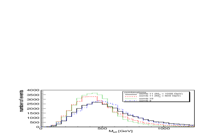
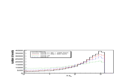
Figure 2: Distributions for $M_{\rm eff}$ (left) and $\Delta\phi_{\ell\ell}$ (right), for combinations 3, 10, and 11 in Tab. 1, which correspond to $Y$ particles with spin 0, $\frac{1}{2}$, and 1, respectively. The plot is based on 35000 parton-level events for each combinations without cuts and detector effects, and using the mass values $m_{Y}$ = 300 GeV and $m_{X}$ = 100 GeV. For combination 11, two choices of the mass of the t-channel particles are shown, $m_{\hat{Q}}$ = 1000 GeV and 500 GeV.

If $Y^{\pm}$ are vector particles, the $M_{\rm eff}$ and $\Delta\phi_{\ell\ell}$ distributions depend on the mass $m_{\hat{Q}}$ of the particle in the t-channel. For $m_{\hat{Q}}\gg m_{Y}$, the $Y^{+}Y^{-}$ pair production cross section reaches its maximum at larger values of $m_{YY}$ than both the spin-0 and spin-1/2 cases, since the s-channel contribution alone grows monotonically with the center-of-mass energy. In this case, the $M_{\rm eff}$ distribution for vector $Y$ particles will peak at larger values than the other two cases, and the $\Delta\phi_{\ell\ell}$ distribution will be very strongly peaked at $\pi$. On the other hand, Fig. 2 shows that for $m_{\hat{Q}}$ of the same order as $m_{Y}$ the $M_{\rm eff}$ distribution can be similar to either the spin-0 or spin-1/2 cases, depending on the precise value of $m_{\hat{Q}}$. Nevertheless, even for a relatively low value $m_{\hat{Q}}=500\,\,\mathrm{GeV}$ the $\Delta\phi_{\ell\ell}$ distribution is still distinctly different for spin-1 compared to the other spin cases. By using all three observables (3)–(5) in combination one therefore obtains the best discrimination power and can unambiguously distinguish between $s_{Y}=0$, $\tfrac{1}{2}$, and 1.

Similar to $\tanh(\Delta\eta_{\ell\ell}/2)$, also $\Delta\phi_{\ell\ell}$ and $M_{\rm eff}$ are invariant under longitudinal boosts, and thus very well suited for hadron colliders.

It needs to be pointed out that the three variables, $\tanh(\Delta\eta_{\ell\ell}/2)$, $\Delta\phi_{\ell\ell}$ and $M_{\rm eff}$, are primarily sensitive to the spin of the parent particle $Y$, but not of the child particle $X$. Indeed, as can be seen from the numerical results in sections 3.4 and 4, it is very difficult to independently determine the $X$ spin.

3.3 Coupling determination

Experiments at LEP and SLC have determined the couplings of the $Z$ boson to SM fermions with very high precision, in particular by measuring various left-right and forward-backward asymmetries [15].

Similarly, for the class of processes corresponding to Fig. 1, one can in principle try to extract information about the $ZYY$ coupling by constructing a forward-backward asymmetry for $pp\to Y^{+}Y^{-}$ at the LHC. Although the initial $pp$ state is symmetric, the incoming quark for a $q\bar{q}$-initiated process often stems from one of the valence quarks of the protons and thus tends to have a larger momentum than the incoming anti-quark. Therefore one can define the forward direction by the direction of the overall longitudinal boost of an event. However, since we neglect effects from electroweak symmetry breaking in the new physics sector, all combinations in Tab. 1 have parity-even $ZYY$ couplings and the forward-backward asymmetry for $pp\to Y^{+}Y^{-}$ is exactly zero.

On the other hand, the coupling between the incident $q\bar{q}$ pair and $Z$ boson has a parity-odd axial-vector part, which results in the $Y^{+}Y^{-}$ pair being produced with a non-vanishing polarization asymmetry (unless $Y^{\pm}$ are scalars). This polarization asymmetry can be probed through the decay $Y^{\pm}\to\ell^{\pm}X^{0}$, since the interaction responsible for the decay is either left- or right-handed and thus sensitive to the $Y$ polarization, see Tab. 1.

In the center-of-mass frame of the $Y^{+}Y^{-}$ system this leads to a forward-backward asymmetry for the final-state leptons. As mentioned above, in the lab frame the forward direction is defined by the overall boost of an event, which is closely correlated to the direction of the more energetic of the two leptons. Therefore we define the observable given in eq. (6),

$$A_{\ell^{+}\ell^{-}}=\frac{N(E_{\ell^{-}}>E_{\ell^{+}})-N(E_{\ell^{+}}>E_{\ell^{-}})}{N(E_{\ell^{-}}>E_{\ell^{+}})+N(E_{\ell^{+}}>E_{\ell^{-}})}.$$ (6)

The asymmetry is partially washed out by the mass $m_{Y}$, which can cause a spin flip before the $Y$ decays, but we expect a non-vanishing result as long as $m_{Y}\ll\sqrt{s}$.

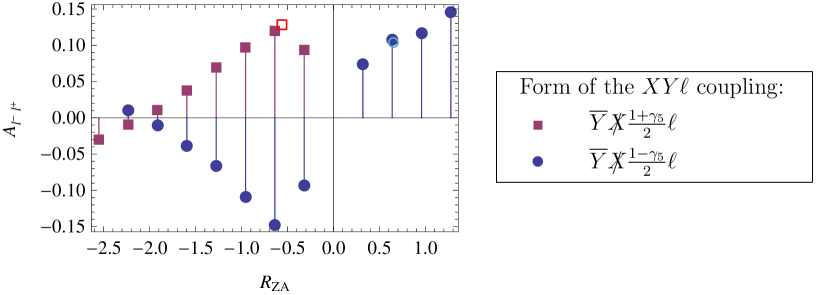
Figure 3: Relationship between the coupling ratio $R_{\rm ZA}=g(ZYY)/e$ and the asymmetry $A_{\ell^{+}\ell^{-}}$, for two different chiralities of the interaction in the $Y^{\pm}\to\ell^{\pm}X^{0}$ decay, where $Y$ is a fermion and $X$ is a vector boson. The combinations 6 and 9 in Tab. 1 are indicated by the open square and circle, respectively. The plot is based on parton-level results without cuts and detector effects, and using the mass values $m_{Y}$ = 300 GeV and $m_{X}$ = 100 GeV.

Eq. 6 is mostly useful for discriminating between combinations with $s_{Y}=\frac{1}{2}$, since scalars do not carry any polarization and lead to a vanishing asymmetry, and there is only one combination with vector $Y$ particles in Tab. 1. The value of $A_{\ell^{+}\ell^{-}}$ is connected to the size of the ratio $R_{\rm ZA}=g(ZYY)/e$ between the $ZYY$ and $\gamma YY$ couplings and to the sign of the $\gamma_{5}$ term in the $XY\ell$ coupling. This is illustrated in Fig. 3 for the case that $Y$ is a fermion and $X$ is a vector boson. As evident from the plot, there is a strong correlation between $R_{\rm ZA}$ and $A_{\ell^{+}\ell^{-}}$, but one can encounter a two- to three-fold ambiguity when trying to determine $R_{\rm ZA}$ from the measured value of $A_{\ell^{+}\ell^{-}}$.

3.4 Numerical results

Using CompHEP we have generated parton-level events for all 11 combinations in Tab. 1 for a center-of-mass energy of $\sqrt{s}=14$ TeV and $m_{Y}=300\,\,\mathrm{GeV}$ and $m_{X}=100\,\,\mathrm{GeV}$. In the following discussion we will assume that the $Y$ and $X$ masses are known from observables like $M_{\rm T2}$, and for simplicity the uncertainty in the mass determination will be neglected.

As explained in the previous section, the observables $\tanh(\Delta\eta_{\ell\ell}/2)$, $M_{\rm eff}$, and $\Delta\phi_{\ell\ell}$, see eqs. (3)–(5) can be used to determine the spin $s_{Y}$ of the parent particle $Y$. We have checked this by performing a 5-bin $\chi^{2}$ analysis for a sample of 5000 events for each model combination, assuming Poisson statistics for the statistical error. Table 3 shows the results for combinations 3 (with scalar $Y$), 10 (with fermion $Y$), and 11 (with vector $Y$) as examples. For the case of vector $Y$ particles, results for two sample values of the t-channel fermion mass $m_{\hat{Q}}$ are given. As evident from the table, by combining the three observables, one can distinguish all three spin combinations from each other with a significance of more than 18 standard deviations, for the given choice of masses and total event count. This is true even for relatively small values of $m_{\hat{Q}}\sim{\cal O}(0.5\,\,\mathrm{TeV})$.

We have checked that the results are very similar if combinations 3 or 10 are replaced by any of the other combinations with spin-0 or spin-1/2 $Y$ particles, respectively. Furthermore, for any two models with identical $s_{Y}$ the distributions for all three variables are statistically consistent, irrespective of the spin of $X$.

	(model A, model B)
Variable	(3,10)	(3,11) [$M_{\hat{Q}}$=1 TeV]	(3,11) [$M_{\hat{Q}}$=0.5 TeV]	(10,11) [$M_{\hat{Q}}$=1 TeV]	(10,11) [$M_{\hat{Q}}$=0.5 TeV]
$\tanh(\Delta\eta_{\ell\ell}/2)$	19.0	18.6	26.0	2.4	8.0
$M_{\rm eff}$	37.5	3.9	25.1	30.7	9.5
$\Delta\phi_{\ell\ell}$	16.3	21.4	10.7	41.1	29.0
All combined	37.5	18.6	26.0	41.1	29.0

Table 3: $\sqrt{\chi^{2}}$ values for a 5-bin $\chi^{2}$-test to discriminate between pairs of model combinations with different spin of the parent $Y$ particle. The combinations 3, 10, and 11 from Tab. 1 have been chosen as examples of models with $Y$ particles of spin 0, $\frac{1}{2}$, and 1, respectively. Model B is assumed to represent the simulated “data”, while model A is the test hypothesis. The results are based on samples of 5000 parton-level events without cuts and detector effects, and using the input values $m_{Y}$ = 300 GeV, $m_{X}$ = 100 GeV, and $\sqrt{s}$ = 14 TeV.

To discriminate between models with identical $s_{Y}$ but different SU(2) representations of the $Y$ and $X$ particles one can take advantage of the charge asymmetry $A_{\ell^{+}\ell^{-}}$ in (6). As mentioned in the previous section, one cannot obtain a non-zero asymmetry if the $Y$ particles are scalars, and we have confirmed this statement explicitly with our simulation results. However, for $s_{Y}=\frac{1}{2}$, $A_{\ell^{+}\ell^{-}}$ can yield useful information about the structure of the $ZYY$ and $XY\ell$ couplings. Results for the total asymmetry, without cuts or acceptance effects, are given in Tab. 4 for all combinations with fermionic $Y$ in Tab. 1.

Combination from Tab. 1	4	5	6	7	8	9	10
$A_{\ell^{+}\ell^{-}}$	$0.20$	$-0.22$	$0.13$	$0.17$	$-0.18$	$0.10$	$0.20$

Table 4: Values for the asymmetry $A_{\ell^{+}\ell^{-}}$ for combinations with fermionic $Y$ in Tab. 1 based on simulated parton-level events for $m_{Y}$ = 300 GeV, $m_{X}$ = 100 GeV, and $\sqrt{s}$ = 14 TeV.

In general, $A_{\ell^{+}\ell^{-}}$ becomes maximal for events with large values of $\cos\theta^{*}_{\ell\ell}=\tanh(\Delta\eta_{\ell\ell}/2)$ close to 1, $i.\,e.$ when the $Y^{+}Y^{-}$ pair is produced in the forward/backward direction. However, this correlation between $A_{\ell^{+}\ell^{-}}$ and $\tanh(\Delta\eta_{\ell\ell}/2)$ depends to a lesser extent also on spin effects in the decay $Y\to\ell X$ and thus can be markedly different for models with opposite chirality of the $XY\ell$ vertex. As a result, the significance for distinction between such models is increased by performing a binned analysis for the distribution $dA_{\ell^{+}\ell^{-}}/d\tanh(\Delta\eta_{\ell\ell}/2)$. It turns out that the highest sensitivity is obtained by using just two bins.

Table 5 lists the statistical significances for discriminating between any pair of the combinations 4–10 from Tab. 1 based on this observable. Models that have different signs for $A_{\ell^{+}\ell^{-}}$ can be distinguished with more than 20 standard deviations for an signal event sample of 5000 events (bold face numbers in the table).

However, the combinations 4, 7, and 10, as well as 6 and 9, are indistinguishable at the three-sigma level (gray italic numbers in the table). It turns out that also when considering any other variables in eqs. (2)–(5) one cannot achieve a higher significance for discriminating between these models.

		model A
		4	5	6	7	8	9
	5	36
	6	4.9	29
	7	1.6	33	2.9
	8	32	3.5	26	29
	9	6.7	27	1.5	4.7	23
	10	0.3	37	5.8	2.2	33	7.6

Table 5: Statistical significance, in units of standard deviations, for the discrimination between combinations with fermionic $Y$ in Tab. 1 using the differential asymmetry $dA_{\ell^{+}\ell^{-}}/d\tanh(\Delta\eta_{\ell\ell}/2)$. Numbers in bold face indicate a difference of at least 20 standard deviations, while gray italic numbers denote a significance of less than three standard deviations. The results are based on samples of 5000 parton-level events without cuts and detector effects, and using the input values $m_{Y}$ = 300 GeV, $m_{X}$ = 100 GeV, and $\sqrt{s}$ = 14 TeV.

Note that the variable $A_{\ell^{+}\ell^{-}}$ has some sensitivity to distinguish between models which differ only through the spin of the $X$ particle, $i.\,e.$ between combinations 4 and 6, or 7 and 9 in Tab. 1. Assuming a signal sample of 5000 events, as in Tab. 5, a discrimination significance of about five standard deviations can be achieved for these pairs.

3.5 Simulation results

The analysis in the previous section does not take into account detector acceptance and signal selection cuts. To study the influence of these effects on the results we have passed the parton-level events generated by CompHEP [14] through Pythia 6.4 [16] and PGS4 [17]. By including initial-state radiation and parton showering in the Pythia simulation one can furthermore evaluate whether fluctuations of the initial-state transverse momentum might wash out the characteristic features for the model discrimination.

In Ref. [5] it has been shown that the selection cuts

$$N(\ell^{+}) =N(\ell^{-})=1, m_{\ell\ell} >150\,\,\mathrm{GeV}, \max\{p_{\rm T,\ell^{\pm}}\}>40\,\,\mathrm{GeV},\quad\min\{p_{\rm T,\ell^{\pm}}\}>30\,\,\mathrm{GeV},$$

$$\makebox[0.86108pt][l]{$p$}/_{\rm T} >100\,\,\mathrm{GeV}, M_{\rm T2} >100\,\,\mathrm{GeV}, |\makebox[0.86108pt][l]{$\mbox{\bf p}$}/_{\rm T}+{\bf p}_{\rm T,\ell^{+}}+{\bf p}_{\rm T,\ell^{-}}|<100\,\,\mathrm{GeV},$$

$$p_{\rm T,j} <100\,\,\mathrm{GeV}, N_{b} =0,$$ (9)

reduce the SM background rate to about 1.6 fb. Here $N(\ell^{\pm})$ denotes the number of visible leptons $\ell^{\pm}=e^{\pm},\mu^{\pm}$ in the central detector, $N_{b}$ denotes the number of vertex $b$ tags, $m_{\ell\ell}$ is the di-lepton invariant mass, and $p_{\rm T,j}$ refers to the transverse momentum of any reconstructed jet. With these cuts one obtains a selection efficiency for the signal process $pp\to Y^{+}Y^{-}\to\ell^{+}\ell^{-}XX$ between 27% and 40%, depending on the specific type of $Y$ and $X$ particle. As listed in the appendix, this corresponds to measurable signal cross sections between about 1 fb and 200 fb. For concreteness we will assume 5000 observed events, which corresponds to the expected yield of model combination 7 for an integrated luminosity of 200 fb^-1. In comparison, the SM background of about 300 events is small and can be neglected.

	(model A, model B)
Variable	(3,10)	(3,11) [$M_{\hat{Q}}$=1 TeV]	(3,11) [$M_{\hat{Q}}$=0.5 TeV]	(10,11) [$M_{\hat{Q}}$=1 TeV]	(10,11) [$M_{\hat{Q}}$=0.5 TeV]
$\tanh(\Delta\eta_{\ell\ell}/2)$	23.2	20.1	30.6	6.3	10.1
$M_{\rm eff}$	40.0	9.7	24.2	36.8	12.6
$\Delta\phi_{\ell\ell}$	27.2	15.5	6.0	40.7	23.8
All combined	40.0	20.1	30.6	40.7	23.8

Table 6: $\sqrt{\chi^{2}}$ values for a 5-bin $\chi^{2}$-test to discriminate between pairs of model combinations with different spin of the parent $Y$ particle, for a sample of 5000 events passing the detector simulation and selection cuts in eq. (9). The notation and input parameters are the same as in Tab. 3.

		model A
		4	5	6	7	8	9
	5	23
	6	3.3	20
	7	2.0	22	1.6
	8	22	2.1	19	21
	9	3.7	19	1.7	3.3	17
	10	1.3	25	4.1	2.1	23	5.3

Table 7: Statistical significance, in units of standard deviations, for the discrimination between combinations with fermionic $Y$ using $dA_{\ell^{+}\ell^{-}}/d\tanh(\Delta\eta_{\ell\ell}/2)$. The results are based on a sample of 5000 events passing the detector simulation and selection cuts in eq. (9), with notation and input parameters are the same as in Tab. 5.

Tables 6 and 7 summarize the significance for distinguishing between models with different $Y$ spin and with different couplings, assuming 5000 measured events for $\sqrt{s}=14$ TeV, $m_{Y}=300\,\,\mathrm{GeV}$ and $m_{X}=100\,\,\mathrm{GeV}$. Overall, the obtained significances for the spin discrimination are comparable to the parton-level results in Tab. 3, and in a few cases the significance is even higher. This seemingly surprising outcome is related to the fact that we compare the same number of “observed” events in the previous section and in this section, but in the latter case the cuts remove part of the phase space, leaving a higher event yield in the remaining phase-space region.

For the coupling determination one finds that the asymmetry $A_{\ell^{+}\ell^{-}}$ is washed out noticeably by the cuts, leading to substantially reduced significances in Tab. 7 compared to Tab. 5. Nevertheless, models with different sign for $A_{\ell^{+}\ell^{-}}$ can still be distinguished with at least 17 standard deviations.

In summary, for most cases, selection cuts and smearing effects only moderately affect the capability for identifying particle properties with the described observables. Of course the selection cuts reduce the overall event number, which however also depends on the model-dependent total cross section and thus is left as a free parameter here.

4 Comparison with Automated Likelihood Analysis

An alternative approach for the analysis of a new-physics signal is an automated likelihood test for a sample of measured events. With such a computerized procedure it is in general not possible to clearly separate properties like spin and couplings, but it offers the advantage of reaching a higher sensitivity by using the complete event information instead of specific observables. A very appealing realization of an automated likelihood analysis is the Matrix Element Method (MEM) [9, 10], which uses parton-level matrix elements to specify the theoretical model that is compared with the data. The method can be used to measure one or several parameters of the model by finding the maximum of the likelihood for a sample of events as a function of these parameters. As of today, the MEM achieves the most precise determination of the top-quark mass [10] and new-physics particle masses [4].

For each single event, with observed momenta $\textbf{p}_{i}^{\rm vis}$, the MEM defines a likelihood measure that it agrees with a model for a given set of model parameters $\alpha$:

$${\cal P}(\textbf{p}^{\rm vis}_{i}|\alpha) =\frac{1}{\sigma_{\alpha}}\int dx_{1}dx_{2}\,\frac{f_{1}(x_{1})f_{2}(x_{2})}{2sx_{1}x_{2}}\left[\prod_{i\in\text{final}}\int\frac{d^{3}p_{i}}{(2\pi)^{3}2E_{i}}\right]|M_{\alpha}(p_{i})|^{2}\prod_{i\in\text{vis}}\delta(\textbf{p}_{i}-\textbf{p}^{\rm vis}_{i}).$$ (10)

Here $f_{1}$ and $f_{2}$ are the parton distribution functions, $M_{\alpha}$ is the theoretical matrix element, and $\sigma_{\alpha}$ is the total cross section, computed with the same matrix element. The 3-momenta $\textbf{p}_{i}^{\rm vis}$ of the visible measured objects are matched with the corresponding momenta $\textbf{p}_{i}$ of the final state particles in the matrix element, while the momenta of invisible particles (weakly interacting particles, such as the $X$ particle in our case) are integrated over.

For a sample of $N$ events, the combined likelihood is usually stated in terms of its logarithm, which in the large-$N$ limit can be interpreted as a $\chi^{2}$ value,

$$\chi^{2}=-2\ln({\cal L})=-2\sum_{n=1}^{N}\ln{\cal P}(\textbf{p}^{\rm vis}_{n,i}|\alpha),$$ (11)

where $\textbf{p}^{\rm vis}_{n,i}$ are the measured momenta of the $n$th event.

The MEM is particularly useful for signals that cannot be fully reconstructed due to invisible final-state particles, and it can be applied to determine the masses of both $X$ and $Y$ in processes of the type in eq. (1) [4]. Here we will assume that the masses are already known and instead focus on the discrimination between the models in Tab. 1.

Matrix elements for all 11 combinations in the table have been computed with the help of CompHEP and implemented into a private code for performing the phase-space integration in (10). Similar to section 3.4 only parton-level events without cuts have been used in this analysis. Results for model comparisons are listed in Tables 8 and 9.

(model A, model B)
(3,10)	(3,11) [$M_{\hat{Q}}$=1 TeV]	(3,11) [$M_{\hat{Q}}$=0.5 TeV]	(10,11) [$M_{\hat{Q}}$=1 TeV]	(10,11) [$M_{\hat{Q}}$=0.5 TeV]
60	59	61	85	87

Table 8: Statistical significance, in units of standard deviations, for the discrimination between pairs of model combinations with different spin of the parent $Y$ particle, based on the MEM. A sample of 5000 parton-level events without cuts and detector effects has been used. The notation and input parameters are the same as in Tab. 3.

As can be seen from Tab. 8, the MEM achieves a much higher significance for discriminating between combinations with different $s_{Y}$, see Tab. 3 for comparison. This is not surprising since several observables, eqs. (3)–(5), were found to be sensitive to the $Y$ spin, indicating that none of them captures all relevant information. Note also that the results in Tab. 8 do not depend strongly on the unknown mass of the t-channel fermion $\hat{Q}$ for combination 11.

		model A
		4	5	6	7	8	9
	5	30
	6	8.3	25
	7	2.5	29	9.1
	8	30	2.3	27	28
	9	8.6	26	3.0	9.0	27
	10	15	41	22	14	43	20

Table 9: Statistical significance, in units of standard deviations, for the discrimination between combinations with fermionic $Y$ in Tab. 1 based on the MEM. A sample of 5000 parton-level events without cuts and detector effects has been used. The notation and input parameters are the same as in Tab. 5.

The MEM can also distinguish between combinations that all have spin-1/2 $Y$ particles but which differ in the SU(2) representations of $X$ and $Y$, as shown in Tab. 9. It is interesting to note that in most cases the statistical significance achieved by the MEM is comparable to the results obtained with the asymmetry $A_{\ell^{+}\ell^{-}}$ in Tab. 5. An exception is combination 10 which can be distinguished from the other combinations with substantially higher significance using the MEM compared to $A_{\ell^{+}\ell^{-}}$. This implies that the asymmetry $A_{\ell^{+}\ell^{-}}$ captures essentially all measurable information about the $ZYY$ and $XY\ell$ couplings, except for the special case of model 10.

Similar to the results of the previous section, it is found that one cannot discriminate very well between combinations with $Y$ singlets and $Y$ doublets, $i.\,e.$ between 4 and 7, 5 and 8, or 6 and 9. Likewise, the MEM results for the combinations 1, 2, and 3 with scalar $Y$ differ by less than one standard deviation, and thus are completely indistinguishable.

5 Conclusions

This paper presents a comprehensive analysis of new physics processes of the form $pp\to Y^{+}Y^{-}\to\ell^{+}\ell^{-}X^{0}\bar{X}^{0}\,(\ell=e,\mu)$, where $X^{0}$ is stable and weakly interacting, leading to a signature of two opposite-sign same-flavor leptons and missing momentum. To minimize model assumptions, all possible combinations for the spins and weak SU(2) couplings of $X$ and $Y$ have been considered, allowing for spin 0, $\frac{1}{2}$ and 1, and SU(2) iso-singlets, -doublets and -triplets, see Tab. 1.

The signal processes have been analyzed with two different and complementary approaches. The first method is based on specific observables. Concretely, we have studied three variables for the measurement of the spins and one asymmetry for the extraction of information about the couplings of the new particles. Secondly, an automated strategy called the Matrix Element Method has been used, which algorithmically computes a likelihood that a given event sample agrees with some model interpretation supplied in the form of a theoretically calculated matrix element.

It has been found that the spin $s_{Y}$ of the parent particle $Y$ can be determined with high statistical significance, so that a sample of a few hundred signal events is sufficient for discrimination at the 5$\sigma$-level. Furthermore, it was shown that the asymmetry $A_{\ell^{+}\ell^{-}}$ defined in eq. (6) is instrumental in distinguishing between model combinations that all have $s_{Y}=\frac{1}{2}$ but different $Y$ and $X$ couplings. The majority of possible coupling assignments can be differentiated with high significance, but it turns out that for the pairs 4 and 7, 5 and 8, as well as 6 and 9 in Tab. 1 one cannot achieve a $3\sigma$ discrimination with a realistic number of a few thousand events. This is related to the fact that the relationship between the $ZYY$ coupling strength and the observable asymmetry is not monotonic and can involve degenerate solutions. Remarkably, the same model combinations are also difficult to distinguish with the Matrix Element Method, which demonstrates that the asymmetry $A_{\ell^{+}\ell^{-}}$ reflects all relevant information about the couplings of the underlying model.

For $s_{Y}=0$ it is generally impossible to discriminate between cases with different couplings or with different spin of the $X$ particles, due to the absence of spin correlations between the production and decay stages of the process. For $s_{Y}=1$ the coupling structure of the process is essentially fixed by gauge invariance and thus already uniquely known once the vector nature of $Y$ has been determined.

Our findings indicate that even for the challenging case of a process with a short one-step decay chain it is in general possible to separately determine the spins and couplings of the new heavy particles. The results in this paper have been presented for the specific choice of masses $m_{Y}=300\,\,\mathrm{GeV}$ and $m_{X}=100\,\,\mathrm{GeV}$, but we have checked explicitly that the essential features are unchanged for $m_{Y}=200\,\,\mathrm{GeV}$. While the main goal of this study was the development of the theoretical framework and conceptual ideas, we have also performed a fast detector simulation with selection cuts for the suppression of standard model backgrounds and found that qualitatively our conclusions still hold. Nevertheless, a dedicated experimental simulation with a careful evaluation of systematic errors, including the influence of uncertainties in the $Y$ and $X$ masses, would be required to check the viability of our results under realistic conditions.

Appendix: Model cross sections

The following table lists the tree-level parton-level production cross sections $\sigma_{\rm prod}$ for the process $pp\to Y^{+}Y^{-}\to\ell^{+}\ell^{-}X^{0}\bar{X}^{0}\,(\ell=e,\mu)$, for the 11 independent combinations from Tab. 1. Also shown are the measurable cross sections $\sigma_{\rm meas}$ after inclusion of detector effects and the cuts in eq. (9). The cross sections have been computed with CompHEP.

Combination	$\sigma_{\rm prod}$ [fb]	$\sigma_{\rm meas}$ [fb]
1	003.62	001.45
2	008.50	003.36
3	009.65	003.11
4	041.4	011.45
5	041.4	011.70
6	041.4	014.05
7	089.6	025.0
8	029.9	008.47
9	089.6	031.4
10	112	031.2
11 [$M_{\hat{Q}}$=0.5 TeV]	179	048.3
11 [$M_{\hat{Q}}$=1 TeV]	445	137

References

-
[1]
C. G. Lester and D. J. Summers,
Phys. Lett. B 463, 99 (1999);
A. Barr, C. Lester and P. Stephens, J. Phys. G 29, 2343 (2003). -
[2]
W. S. Cho, K. Choi, Y. G. Kim and C. B. Park,
Phys. Rev. Lett. 100, 171801 (2008);
A. J. Barr, B. Gripaios and C. G. Lester, JHEP 0802, 014 (2008);
W. S. Cho, K. Choi, Y. G. Kim and C. B. Park, JHEP 0802, 035 (2008);
D. R. Tovey, JHEP 0804, 034 (2008);
H. C. Cheng and Z. Han, JHEP 0812, 063 (2008);
A. J. Barr, B. Gripaios and C. G. Lester, JHEP 0911, 096 (2009). -
[3]
G. Polesello and D. R. Tovey,
JHEP 1003, 030 (2010);
K. T. Matchev and M. Park, arXiv:0910.1584 [hep-ph];
P. Konar, K. Kong, K. T. Matchev and M. Park, Phys. Rev. Lett. 105, 051802 (2010);
T. Cohen, E. Kuflik and K. M. Zurek, JHEP 1011, 008 (2010). -
[4]
J. Alwall, A. Freitas and O. Mattelaer,
AIP Conf. Proc. 1200, 442 (2010);
P. Artoisenet, V. Lemaitre, F. Maltoni and O. Mattelaer, arXiv:1007.3300 [hep-ph];
J. Alwall, A. Freitas and O. Mattelaer, in preparation. - [5] A. J. Barr, JHEP 0602, 042 (2006).
-
[6]
W. S. Cho, K. Choi, Y. G. Kim and C. B. Park,
Phys. Rev. D 79, 031701 (2009);
D. Horton, arXiv:1006.0148 [hep-ph]. -
[7]
M. R. Buckley, H. Murayama, W. Klemm and V. Rentala,
Phys. Rev. D 78, 014028 (2008);
M. R. Buckley, S. Y. Choi, K. Mawatari and H. Murayama, Phys. Lett. B 672, 275 (2009). - [8] G. L. Kane, A. A. Petrov, J. Shao and L. T. Wang, J. Phys. G 37, 045004 (2010).
-
[9]
K. Kondo,
J. Phys. Soc. Jap. 57, 4126 (1988),
J. Phys. Soc. Jap. 60, 836 (1991);
R. H. Dalitz and G. R. Goldstein, Phys. Rev. D 45, 1531 (1992). -
[10]
B. Abbott et al. [D0 Collaboration],
Phys. Rev. D 60, 052001 (1999);
V. M. Abazov et al. [D0 Collaboration], Nature 429, 638 (2004);
A. Abulencia et al. [CDF Collaboration], Phys. Rev. D 74, 032009 (2006);
V. M. Abazov et al. [D0 Collaboration], Phys. Rev. D 78, 012005 (2008);
T. Aaltonen et al. [CDF Collaboration], Phys. Rev. Lett. 101, 252001 (2008);
F. Fiedler, A. Grohsjean, P. Haefner and P. Schieferdecker, Nucl. Instrum. Meth. A 624, 203 (2010). -
[11]
G. L. Bayatian et al. [CMS Collaboration],
J. Phys. G 34, 995 (2007);
G. Aad et al. [ATLAS Collaboration], arXiv:0901.0512 [hep-ex]. - [12] S. P. Martin, in “Perspectives on supersymmetry II,” ed. G. L. Kane, World Scientifc, Singapore (2010), pp. 1–153 [hep-ph/9709356].
-
[13]
T. Appelquist, H. C. Cheng and B. A. Dobrescu,
Phys. Rev. D 64, 035002 (2001);
B. A. Dobrescu and E. Pontón, JHEP 0403, 071 (2004);
G. Burdman, B. A. Dobrescu and E. Pontón, JHEP 0602, 033 (2006). - [14] E. Boos et al. [CompHEP Collaboration], Nucl. Instrum. Meth. A 534, 250 (2004).
- [15] S. Schael et al., Phys. Rept. 427, 257 (2006).
- [16] T. Sjöstrand, S. Mrenna and P. Z. Skands, JHEP 0605, 026 (2006).
- [17] J. Conway, PGS 4, http://www.physics.ucdavis.edu/~conway/research/software/pgs/pgs4-general.htm.
- [18] L. Randall and D. Tucker-Smith, Phys. Rev. Lett. 101, 221803 (2008).