Understanding quantum interference in General Nonlocality

Abstract

In this paper we attempt to give a new understanding of quantum double-slit interference of fermions in the framework of General Nonlocality (GN) [J. Math. Phys. 49, 033513 (2008)] by studying the self-(inter)action of matter wave. From the metric of the GN, we derive a special formalism to interpret the interference contrast when the self-action is perturbative. According to the formalism, the characteristic of interference pattern is in agreement with experiment qualitatively. As examples, we apply the formalism to the cases governed by Schrödinger current and Dirac current respectively, both of which are relevant to topology. The gap between these two cases corresponds to the fermion magnetic moment, which is possible to test in the near future. In addition, a general interference formalism for both perturbative and non-perturbative self-actions is presented. By analyzing the general formalism we predict that in the nonperturbative limit there is no interference at all. And by comparison with the special formalism of Schrödinger current, the coupling strength of self-action in the limit is found to be $\infty$. In the perturbative case, the interference from self-action turns out to be the same as that from standard approach of quantum theory. Then comparing the corresponding coefficients quantitatively we conclude that the coupling strength of self-action in this case falls in the interval $[0,1]$.

I Introduction

Up to date, the experiments on quantum double-slit interference/diffraction have been realized with a series of single, separate fermions (electrons, neutrons etc.)  Claus  Tono  links  Zeil . A logical inference is that the interference pattern is created by each single particle interfering with itself. The given explanation is the Schrödinger description Ahar using the analogy to the optical Young’s experiment and Huygens-Fresnel principle. In this picture the fermion, one and the same quantum entity, has to be viewed as a local particle in the source and on the screen, but as a true matter wave for the propagating procedure in between Nairz . Accordingly, the interference fringe is believed to be produced by the superposition of the waves from the two slits. It confuses us by introducing classically split paths to a matter wave. So far quantum interference has been always explained by utilizing a somewhat classical wave. In this paper we employ a realistic quantum nonlocal wave to describe the whole interference procedure, and the very same quantum entity can be viewed as a particle only when its charge(or one of other quantum numbers) is detected. Our nonlocal method and the given explanation differ in that the given explanation requires separate paths for a matter wave, whereas our nonlocality needs only one spreading path.

The aim of this paper is to apply the theory of nonlocality Wanng to the nonlocal phenomenon—double-slit interference. There are other works  Ahar  Pope specifying the relationship between the nonlocality and the interference from different perspectives. In the reference Ahar the authors attempt to link a set of locally measurable operators (observables) with each nonlocal procedure occurring between the source and the screen. These operators are designed to be sensitive to the relative phase of two slits, and to be involved in a kind of nonlocal interaction by satisfying the nonlocal Heisenberg equation of motion. In this sense the intermediate process of double-slit interference is explained on a somewhat deterministic basis, so in principle, can be measured too. Significantly, the authors put forth and explain clearly the important fact that there are two kinds of nonlocality: one is the well-known correlation born from the violation of Bell-inequality concerning the Hilbert-space structure; the other is relating to the typical issue of double-slit experiment—in which the relative phase of two slits cannot be observed locally—it is called a dynamical nonlocality. The latter is the objective of this paper.

Different from other explanations to the quantum interference, in this work we focus our attention on the performance of the matter wave rather than the particles’ position. We hold the point of view that the detection of the position of a quantum particle relies on one kind of its charges/(or one of its quantum numbers), whereas the detection of a wave usually depends on the interferenc/defraction it produces. For a quantum entity, its wave is like a wing around the charge(s), forming an inseparable entirety. In a sense it is the stochastic behavior of the charge(s) in the wing that makes us realize the nonlocality. When an interaction happens to the quantum particle, both the ”wing” and the charge(s)/(quantum numbers) are involved. In quantum mechanics and conventional quantum field theory (CQFT), only the charges/(quantum numbers) are mostly emphasized, whereas the low energy limit–when the wave characteristic dominates the processes—has rarely been considered. The two-slit interference is a paradigm to display wave’s nonlocality. And this kind of nonlocality cannot be completely described solely by any conventional equation of motion, such as Schrödinger equation or Dirac equation.

The starting point of this paper is the principle of the GN: A quantum wave always remains an entirety (in a special complex reference frame, this entirety is plane wave) regardless of interactions/observations (from the point of view of quantum field, we regard any observation as a kind of interaction). This principle has been applied to the metrics corresponding to complex spaces to derive the equation of motion for fermions and the field equation for bosons Wanng . Here we apply this principle to the wave covering the two slits. Between the slits, namely the grating, is the singularity mentioned in  Wanng . Since this wave keeps entirety in the whole intermediate process, there is a moment when the wave breaks itself at one side of the slits and simultaneously merges together at the other side of the slits. At this very moment the wave forms a loop in the 3-dimension configuration space [fig.1c]. We describe this loop using the metric of GN and the Action form in CQFT. The terminology of Action in CQFT provides direct relevance to topology.

Since each intermediate process of interference involves only one fermion’s wave, we recognize that the two-slit interference phenomenon is intrinsically nonlocal. Therefore the extended (nonlocal) wave must interact with itself around the slits (the grating acts as a singularity). We name such interaction as self-(inter)action henceforth and describe it by fermion’s current. This current-self-action is found to reside in the metric of General Nonlocality (GN)Wanng , which in the perturbative limit is equivalent to a phase factor—an exponential of partial Action $S=\int\mathscr{L}\/d^{4}x$. The interaction term in the Lagrangian $\mathscr{L}$ now becomes self-action in concept. The metric interpretation is assumed available in our prescription even when the self-action is nonperturbative. Our purpose is to understand the possible new effects suggested by the self-action and non-perturbation. The self-action is new for conventional quantum theory.

The remaining parts of the paper are arranged as follows. In section II we derive a special formalism for interference phenomenon by starting from the metric of GN and by considering only a classically thin "path" for a wave [fig.2]. The formalism is relevant to the Action in CQFT in the case of perturbative self-action. In Secs. III-IV the above special formalism is applied to Schrödinger current and Dirac current, and the relevant topology is discussed. Sec. V is dedicated to the general formalism for interference where an extended "path" [fig.2](all the possibilities of complex/configuration space) is involved. In Sec. VI we estimate the strengths of self-action in different cases by analyzing relevant experiments and comparing our results with conventional approaches of quantum theory. Finally summary and remarks are presented.

II The special formalism for interference phenomenon

The theory of GN Wanng states that a spatially-extended quantum wave is a nonlocal entity as an entirety—”a point of complex space”. There always exists a local complex reference frame in which the matter wave looks like a plane wave (The wave is observed by another fermion or by itself), no matter the existence of interactions/observations. Sometimes the interaction/observation may be caused/performed by the change of configurations. For example, while a wave passing through the double-slit plane, the wave is to some extent interacting with the verges of the slits. According to the principle of nonlocality, we infer that at any moment the wave exists as an entirety, unlike the usual assumption that the wave is split into two parts before they finally meet at a point on the screen. So even if the splitting actually happens, it occurs after the wave fronts having met and merged on the other side of the slit-plane [fig. 1]. We interpret this kind of integrity (entirety) by transforming the integral over the whole 4-dimensional space—used in metric of General Nonlocality[see eq. (2.5)]—to a line integration along one spreading path [see eq. (3.1)].

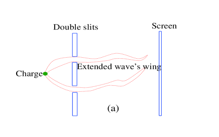
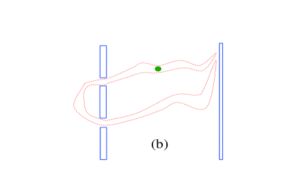
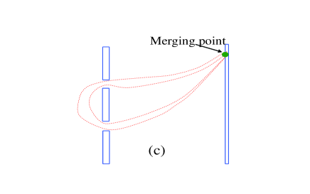
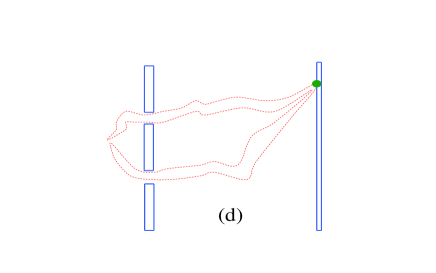
Figure 1: We use scheme diagrams (1a)-(1d) to illustrate the procedure of a matter wave evolving from one side of two-slit-barrier to another side, until its two "ends" meet and merge on screen. Here the realistic wave’s scale is used, with only a few wavelengths involved.

Accordingly, we start with the metric for the fermion fields,

$$G(\bar{\psi},\psi)=d\psi^{\alpha}A_{\alpha\bar{\beta}}d\bar{\psi}^{\beta}\text{ ,}$$ (2.1)

here we will use the projected form of local wave function (in the paper  Wanng a projection was used to project the complex space to a flat subset $d\psi^{\alpha}\rightarrow\psi^{\alpha}$, to enable the wave function observable for a real observer). And we employ the approximate metric tensor as

$$(A_{\alpha\bar{\beta}})_{4\times 4}=\gamma_{0}+\gamma_{0}\gamma^{\mu}A_{\mu}\text{ .}$$ (2.2)

Combining the above two equations yields

$$G(\bar{\psi},\psi)=\bar{\psi}\psi+j^{\mu}A_{\mu}\text{ ,}$$ (2.3)

$\tilde{\psi}=\{\psi^{1},\psi^{2},\psi^{3},\psi^{4}\}$ is a four-component spinor, and $j^{\mu}=\bar{\psi}\gamma^{\mu}\psi$, $\bar{\psi}=\psi^{\dagger}\gamma_{0}$. This projected form actually makes the metric tensor in a quasi-flat space—the usual quantum-mechanical Hilbert space. For a function $\psi(\vec{x},t)$ already projected onto flat space, in experiment however, it is impossible to know its value at each point $\vec{x}$. So an integral should be performed at the right hand side to sum over all the possibilities (we have omitted this integral in Wanng for convenience, since performing the variation for equation of motion is not affected by this omission), the expression (2.3) alters to

$$G(\bar{\psi},\psi)=\int\bar{\psi}\psi d^{3}x+\int j^{\mu}A_{\mu}d^{3}x\text{ .}$$ (2.4)

As from eq. (8.8) to eq. (8.9) in Wanng , by analyzing the dimension we note that in the second term of the last equation (2.4) there lacks a coordinate dimension in comparison with the first term. In the natural unit where coupling constant $e=1$, if assuming the first term $\int\bar{\psi}\psi d^{3}x=1$, then $\psi$ or $\bar{\psi}$ has the dimension of $[L^{-\frac{3}{2}}]$, here we use $[~{}~{}]$ to denote the dimension of a quantity and $[L]$ the dimension of length. As for the second term, $[A_{\mu}]=[L^{-1}]$ and $[j^{\mu}]=[\bar{\psi}][\psi]=[L^{-3}]$ with obviously $[d^{3}x]=[L^{3}]$, so in total the dimension of $\int j^{\mu}A_{\mu}d^{3}x$ is $[L^{-1}]$. This validates the above judgement. The discrepancy of the dimensions is caused by the projection aforementioned. To remedy the unequal dimensions of the two terms and according to our experience of treating the Schrödinger equation with a nonlocal interaction potential WanngB , we add a line integral to the second term, with an imaginary number $i$ beforehand as did formerly,

$$G(\bar{\psi},\psi)=\int\bar{\psi}\psi d^{3}x+i\int j^{\mu}A_{\mu}d^{4}x\text{ .}$$ (2.5)

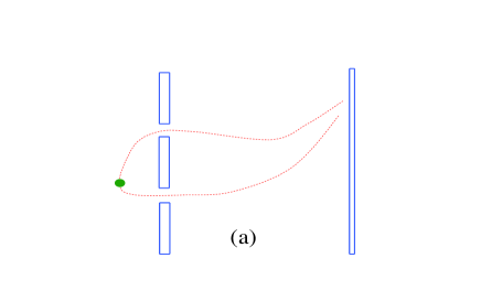
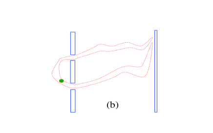
Figure 2: Illustrating the meaning of "thin" path and "spreading" path, which concern the different abstract volumes in the configuration space.

We recognize that while the (self-)interaction $A^{\mu}$ is very weak (perturbative), the above expression associates with the phase factor $e^{iS}$ by

$$G(\bar{\psi},\psi)=1+i\int j^{\mu}A_{\mu}d^{3}x\,\text{d}t=1+i\int\mathscr{L}_{I}\/d^{4}x\sim e^{iS_{I}}\text{ ,}$$ (2.6)

in which $\int\psi^{*}\psi d^{3}x=1$ is applied and the Action form $S_{I}=\int\mathscr{L}_{I}\/d^{4}x$ is understood, where $\mathscr{L}_{I}=j^{\mu}A_{\mu}$ is interaction Lagrangian density (Later on we use the same form to express the self-action.). From eq. (2.6) we realize that the physical meaning of $G(\bar{\psi},\psi)$ (after projection) is linked with the infinitesimally nonlocal evolution of the wave state.

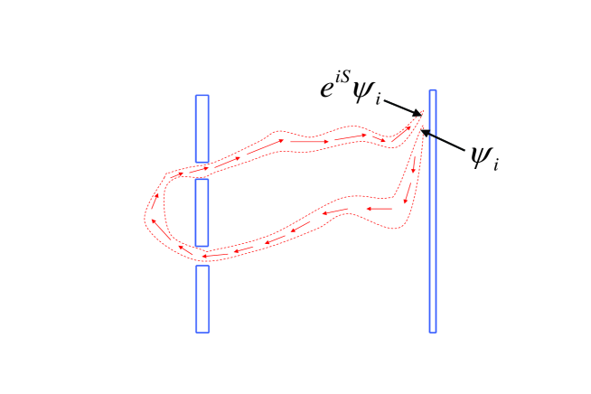
Figure 3: At the merging point on the screen, $e^{iS}\psi_{i}$ meets $\psi_{i}$.

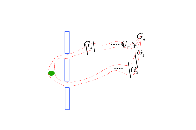
Figure 4: Illustrating how the successive $G_{n}(\bar{\psi},\psi)^{\prime}s$ yield a loop expression.

According to Feynman’s statement FeynA , a path contributes to wave-function with a phase proportional to the action $S$,

$$\phi[x(t)]=\text{const }e^{i\,S[x(t)]/\hbar}\text{ ,}$$ (2.7)

hereafter we use natural unit by letting $\hbar=1$. Thus the wave $\psi_{i}(x)$ evolving from one point $x$ infinitesimally to another point $x+dx$ along the same (thin) path may be expressed by the following form,

$$\psi_{f}(x+dx)=G(\bar{\psi},\psi)\,\psi_{i}=e^{iS_{\bigtriangleup}}\psi_{i}\text{ ,}$$ (2.8)

whereby the volume $d^{3}x\,$d$t$ in the integral $i\int j^{\mu}A_{\mu}d^{4}x$ of $S$ is assumed to be infinitesimal, and the corresponding $S$ is denoted by $S_{\bigtriangleup}$. So at the merging point on the screen, the $e^{iS}\psi_{i}$ meets $\psi_{i}$ [fig.3], with the merging wave as

$$\psi_{\text{merging}}=\psi_{i}+e^{iS}\psi_{i}\text{ ,}$$ (2.9)

where $S=\oint S_{\bigtriangleup}$ forming a loop [fig.4],

$$e^{iS}={\lim_{n\rightarrow\infty}}e^{iS_{\bigtriangleup_{n}}}\cdot\cdot\cdot e^{iS_{\bigtriangleup_{1}}}={\lim_{n\rightarrow\infty}}G_{n}(\bar{\psi},\psi)\cdot\cdot\cdot G_{1}(\bar{\psi},\psi)\text{ .}$$ (2.10)

A more general form of eq. (2.10) will be found in the latter part. This equation is just the special case with only one thin path involved for a wave. The eq. (2.9) gives the probability of finding the fermions by

$$\mid\psi_{i}+e^{iS}\psi_{i}\mid^{2}=\mid e^{-iS/2}\psi_{i}+e^{iS/2}\psi_{i}\mid^{2}=4\cos^{2}\frac{S}{2}\mid\psi_{i}\mid^{2}\text{ ,}$$ (2.11)

which is very the general Cosine form from experimental interference fringes for fermions Tono . It’s known that if the Action form $S_{I}$ contains a conventional kinetic part like $S_{\text{k}}=\int\mathscr{L}_{\text{k}}\/d^{4}x=\int\bar{\psi}(i\not\partial-m)\psi\/d^{4}x\sim\int\frac{\vec{p}^{2}}{2m}\/dt$ (the last step holds for low velocity, $\frac{\mid\vec{\upsilon}\mid}{c}\sim 0$), the $\cos^{2}\frac{S}{2}$ in eq. (2.11) could coincide with conventional approach  FeynA Gli Bar . We leave the discussion of this part implicit here. As for the consistency of lacking this part in $S_{I}$, please refer to the argument following eq. (5.7) and Sec.VI. In Secs. III and IV we will show that it is almost identical to use Schrödinger current or to use Dirac current in the Action form $S$.

III The Schrödinger current—its selfaction and topology

In sense of nonlocalityWanng , at each (arbitrary) moment the wave exists as an entirety, not as usually assumed that the wave has been split into two parts by slit-plane before they finally meet at a point on the screen. Thus far we have admitted that even if the splitting actually happen, they must occur when the wave fronts having met and merged on the other side of the slit-plane [fig.1d]. So we arrive at the conclusion that there is at least one moment the wave shapes itself to form a loop in three-dimension configuration space. This very loop yields the following topological description.

We can go one step further from eq. (2.6) if the self-action has the form like QED,

$$G(\bar{\psi},\psi)=e^{iS}=e^{i\int j_{\mu}A^{\mu}d^{4}x}=e^{iq\int ds_{\mu}A^{\mu}}\text{ ,}$$ (3.1)

by using the relation

$$\int j_{\mu}A^{\mu}d^{4}x=\int\frac{\rho(x)ds_{\mu}}{dt}A^{\mu}d^{4}x=q\int ds_{\mu}A^{\mu}\text{ ,}$$ (3.2)

where $q$ is the charge of the fermion. Please caution that $s_{\mu}$ is born from a current and it is allowed to have some inner structure. If the current is induced by an electron then $q=e=1$ in our default choice. For a general current, $q$ may just be a constant. Moreover, there should exist another charge $q^{\prime}$ in $A^{\mu}$, which will be used later. Reiterating the argument at the beginning of this section, we note that the summing up line-integral should be a loop form, which renders eq. (3.1) to have the following form

$$e^{iS}={\lim_{n\rightarrow\infty}}G_{n}(\bar{\psi},\psi)\cdot\cdot\cdot G_{1}(\bar{\psi},\psi)=e^{iq\oint ds_{\mu}A^{\mu}}\text{ .}$$ (3.3)

Since the intermediate process of each event in interference involves only one fermion’s wave, we can safely infer that the extended (nonlocal) wave must interact with itself around the slits (the grating between the slits forming a singularity). We will interpret this self-action in analogy to the current-current coupling in weak interaction  Fermi , like the form $j_{\mu}j^{\mu}$ apart from a coupling constant. Accordingly the immediate conclusion is

$$A^{\mu}\sim j^{\mu}\text{ , for }A^{\mu}\text{ in eq.(3.3).}$$

We prefer the current form $j^{\mu}=(\rho,\mathbf{J})$ to appear in the line integration eq. (3.3), since it has intriguing inner structures, and could be a potential observable as well.

Now let’s consider a type of self-action regardless of temporal component. Since there is no instantaneous self-action relating to the local charge $q$ (As for the case of self-action, there is at most one point-wise charge present, which is understood to be local and inseparable), we infer $A^{0}=0$. However, since the 3-dimensional current $\mathbf{J}$ is intrinsically nonlocal, its self-action is naturally allowed to occur. Under these justifications, the eq. (3.3) reduces to

$$e^{iS}=e^{i\,q\oint d\mathbf{x}\cdot\mathbf{A}}\sim e^{i\,q\oint d\mathbf{x}\cdot\mathbf{J}}\text{ .}$$ (3.4)

The following Schrödinger current is our objective in this section,

$$\mathbf{A\sim J}=-\frac{i}{2m}[\varphi^{*}(x)\vec{\nabla}\varphi(x)-(\vec{\nabla}\varphi^{*}(x))\varphi(x)]\text{ ,}$$ (3.5)

in the Sec. IV we will show that Dirac current $j^{\mu}=\bar{\psi}(x)\gamma_{\mu}\psi(x)$ behaves in a similar way. The current in eq. (3.5) has an alternative form  WanngA

$$\mathbf{J}=\frac{\rho}{m}\mathbf{\tilde{J}}\text{ }$$,

,

.

(3.6)

Note that there is a dimension [$L^{2}$] difference between $\mathbf{J}$ and $\mathbf{\tilde{J}}$ (for [$\mathbf{J}$]=[$L^{-3}$], [$\mathbf{\tilde{J}}$]=[$L^{-1}$]), and likewise between $j^{\mu}$ and $A^{\mu}$, so we refine the relation $A^{\mu}\sim j^{\mu}$ as $\mathbf{A}=\mathbf{\tilde{J}}$. Consequently, the eq. (3.4) becomes

$$e^{iS}=e^{i\,q\,q^{\prime}\oint d\mathbf{x}\cdot\mathbf{\tilde{J}}}\text{ ,}$$ (3.7)

with $q^{\prime}$ also from the current $\mathbf{J}$.

To study the topology of the current, let’s decompose the wave functions in the above eq. (3.6) as follows

$$\varphi(x)=\phi_{1}+i\phi_{2}\text{ ,}$$

(3.8)

and substituting them back to the eq. (3.6), one has

$$\tilde{J}_{\mu}=\frac{\phi_{1}\partial_{\mu}\phi_{2}-\phi_{2}\partial_{\mu}\phi_{1}}{\phi_{1}^{2}+\phi_{2}^{2}}\text{ ,}$$ (3.9)

furthermore making $n_{1}=\frac{\phi_{1}}{\sqrt{\phi_{1}^{2}+\phi_{2}^{2}}},n_{2}=\frac{\phi_{2}}{\sqrt{\phi_{1}^{2}+\phi_{2}^{2}}},$ yields

$$\tilde{J}_{\mu}=\varepsilon_{ab}n^{a}\partial_{\mu}n^{b}\text{ , }a\text{, }b=1,2\text{.}$$ (3.10)

According to Gauss-Bonnet formula in differential geometry  Chern , the integral of the above vector gives rise to an integer multiplied with constant $2\pi$

$$\oint\tilde{J}_{\mu}dx^{\mu}=2\pi k_{i},\text{ }k_{i}\text{ is an integer,}$$ (3.11)

substituting it into eq. (3.7), one obtains

$$e^{iS}=e^{i\,q\,q^{\prime}\oint d\mathbf{x}\cdot\mathbf{\tilde{J}}}=e^{i\,q\,q^{\prime}\,2\pi\,k_{i}}\text{ ,}$$ (3.12)

here the quantity $q\,q^{\prime}$ plays a role in expressing the strength of the self-action, just as the coupling constants in gauge theory for quantum fields. Substituting the form of $S$ in eq. (3.12) into eq. (2.11) one finds that the width of the interference fringes is determined by the quantity $q\,q^{\prime}$. In turn, the coupling strength $q\,q^{\prime}$ can also be deduced from the interference pattern. We will further investigate the value of $q\,q^{\prime}$ in sect. VI.

IV From Dirac current to Schrödinger current

We have discussed the relationship between the current and its topological properties starting from the simplest case of Schrödinger current. To make our argument more general, we should guarantee the Dirac current includes the Schrödinger current as a special case. In what follows we briefly derive the Schrödinger current from Dirac current. The Dirac equation is

$$i\frac{\partial}{\partial t}\psi(x)=[\vec{\alpha}\cdot(-i\vec{\nabla}-e\vec{A})+eA_{0}+m\beta]\psi(x)\text{ ,}$$ (4.1)

where $\alpha_{\kappa}=\left(\begin{array}[]{cc}0&\sigma_{\kappa}\\ \sigma_{\kappa}&0\end{array}\right)$ and $\beta=\left(\begin{array}[]{cc}1&0\\ 0&-1\end{array}\right)$. From the equation one has obtained the conserved current as follows  Pes ,

$$J_{\mu}=\bar{\psi}(x)\gamma_{\mu}\psi(x)=(\rho,\mathbf{J})\text{ ,}$$ (4.2)

where $\gamma_{0}=\beta=\left(\begin{array}[]{cc}1&0\\ 0&-1\end{array}\right)$ and $\gamma^{k}=\beta\alpha_{k}=\left(\begin{array}[]{cc}0&\sigma_{\kappa}\\ -\sigma_{\kappa}&0\end{array}\right)$. Now we attempt to transform the above eq. (4.2) to Schrödinger current form eq. (3.5).

To proceed, let’s recall the large component method that we have used in eqs. (9.13)~(9.16) of  Wanng . The eq. (9.14) is

$$\psi=\left(\begin{array}[]{c}\psi_{1}\\ \psi_{2}\\ \psi_{3}\\ \psi_{4}\end{array}\right)=\left(\begin{array}[]{c}\psi_{a}\\ \psi_{b}\end{array}\right)\text{ ,}$$ (4.3)

with $\psi_{a}$ being the large component and $\psi_{b}$ the small component, $\psi_{b}$ can be interpreted as

$$\psi_{b}=\frac{\vec{\sigma}\cdot(-i\vec{\nabla}-e\vec{A})}{2\,m}\psi_{a}=\frac{\vec{\sigma}\cdot(\vec{P}-e\vec{A})}{2\,m}\psi_{a}\text{ ,}$$

(4.4)

Now we separately substitute the above approximation into eq.(4.2), to get the approximate form of $\rho$ and $\mathbf{J}$. It yields

$$\rho=\psi^{\dagger}\psi=(\psi_{a}^{\dagger},\psi_{b}^{\dagger})\left(\begin{array}[]{c}\psi_{a}\\ \psi_{b}\end{array}\right)\sim\psi_{a}^{\dagger}\psi_{a}\text{ ,}$$ (4.5a)

$$\mathbf{J}=(\psi_{a}^{\dagger},\psi_{b}^{\dagger})\left(\begin{array}[]{cc}0&\vec{\sigma}\\ \vec{\sigma}&0\end{array}\right)\left(\begin{array}[]{c}\psi_{a}\\ \psi_{b}\end{array}\right)=\psi_{b}^{\dagger}\vec{\sigma}\psi_{a}+\psi_{a}^{\dagger}\vec{\sigma}\psi_{b}$$

(4.5b)

then employing the relation among the components of $\vec{\sigma}$,

$$\sigma^{j}\sigma^{k}=\delta^{jk}+i\varepsilon^{jkl}\sigma^{l}\text{ ,}$$ (4.6)

we can obtain

$$\vec{\sigma}\cdot(-\vec{P})\psi_{a}^{\dagger}\vec{\sigma}\psi_{a}+\psi_{a}^{\dagger}\vec{\sigma}\vec{\sigma}\cdot\vec{P}\psi_{a}$$

(4.7a)

$$\psi_{a}^{\dagger}\vec{A}\cdot\vec{\sigma}\,\vec{\sigma}\psi_{a}+\psi_{a}^{\dagger}\vec{\sigma}\,\vec{A}\cdot\vec{\sigma}\psi_{a}$$

(4.7b)

So the eq.(4.5b) becomes

$$\mathbf{J}=-\frac{i}{2m}[\psi_{a}^{\dagger}\vec{\nabla}\psi_{a}-(\vec{\nabla}\psi_{a}^{\dagger})\psi_{a}]+\frac{1}{2m}[(\vec{\nabla}\psi_{a}^{\dagger})\times\vec{\sigma}\psi_{a}-\psi_{a}^{\dagger}\vec{\sigma}\times(\vec{\nabla}\psi_{a})]\text{ ,}$$ (4.8)

in which $\psi_{a}^{\dagger}$ is a $2\times 1$ matrix. The above equation has already taken the shape of Schrödinger current, apart from an additional term $(\vec{\nabla}\psi_{a}^{*})\times\vec{\sigma}\psi_{a}-\psi_{a}^{*}\vec{\sigma}\times(\vec{\nabla}\psi_{a})$ (we name this part as spin current) due to the inclusion of spin $\vec{\sigma}$. For the interference pattern induced by single fermions, the fringes should have an additional shift induced by the self-action of spin $\vec{\sigma}$, just like the contribution of $\vec{\sigma}_{i}\cdot\vec{\sigma}_{j}$ in potential model WanngB .

The spin current can be further transformed into

$$\mathbf{J}_{\sigma}=\frac{1}{2m}[(\vec{\nabla}\psi_{a}^{*})\times\vec{\sigma}\psi_{a}-\psi_{a}^{*}\vec{\sigma}\times(\vec{\nabla}\psi_{a})]=\frac{1}{2m}\vec{\nabla}\times(\psi_{a}^{*}\vec{\sigma}\psi_{a})\text{ ,}$$ (4.9)

which just coincides with the Ampere law expressed in Maxwell equations

$$\vec{\nabla}\times\vec{B}=\vec{j}+\frac{\partial\vec{E}}{\partial t}\text{ .}$$ (4.10)

The eq. (4.9) cannot be further written as in eq. (3.10) which is convenient for directly discussing topology. This term however, formally relates to topology in a manner named Aharonov-Casher (AC) AC effect, though the physics here is irrelevant to AC effect. Likewise the eq. (3.4) is formally similar to Aharonov-Bohm (AB) effect  AB . From eq. (4.10) we realize that the term $\psi_{a}^{*}\vec{\sigma}\psi_{a}$ is just the magnetic moment of a fermion. While the interference happens, it surely accumulates its effect on the interference pattern due to eq. (3.5). Based on the experience of comparing AC effect ACE and AB effect ABE , this shift from $\psi_{a}^{*}\vec{\sigma}\psi_{a}$ should be less than 0.1 percent of the original. Thus in nonlocality, the strength of coupling $\vec{\sigma}_{i}\cdot\vec{\sigma}_{j}$ may have the order of magnitude $1/1000$ as the self-action in eq.(3.12). We expect this tiny interference effect could be tested by experiment, e.g. via comparing the interference patterns induced by single protons and single neutrons, if possible.

V The general formalism for quantum interference

This section is dedicated to giving a general expression of eq. (2.10), ${\lim_{n\rightarrow\infty}}G_{n}(\bar{\psi},\psi)\cdot\cdot\cdot G_{1}(\bar{\psi},\psi)$, which helps us to get the interference terms like those in eq. (2.9), $\psi_{\text{merging}}=\psi_{i}+(sth)\psi_{i}$. Here the general form means that we should take into account the diffusive and extended (spreading) characteristic of the wave. This characteristic is interpreted in Feynman path integral by performing the integral with respect to the measure $[D\bar{\psi}][D\psi]$, which we will use for reference. So, the expression we will treat is

$${\lim_{n\rightarrow\infty}}\int[D\bar{\psi}][D\psi]G_{n}(\bar{\psi},\psi)\cdot\cdot\cdot G_{1}(\bar{\psi},\psi)\text{ .}$$ (5.1)

The calculation doesn’t belong to Feynman path integral unless the self-action is perturbative, though it shares the same form as Feynman integral  Explain . Here we first review the treating of perturbative case, then cope with the non-perturbative case.

Let’s rewrite the integral eq. (5.1) explicitly in a piece-wise manner by substituting the eq. (2.1),

$${\lim_{n\rightarrow\infty}}\frac{1}{N}\int[D\bar{\psi}_{n}][D\psi_{n}]\cdot\cdot\cdot[D\bar{\psi}_{1}][D\psi_{1}](d\psi_{n}^{\alpha}A_{\alpha\bar{\beta}}d\bar{\psi}_{n}^{\beta})\cdot\cdot\cdot(d\psi_{1}^{\alpha}A_{\alpha\bar{\beta}}d\bar{\psi}_{1}^{\beta})\text{ ,}$$ (5.2)

in which we use the convenient formalism before projection—like in Ref. Wanng , each $d\psi_{n}$ standing for the local wave function for an infinitesimal short scale in complex space, and $d\bar{\psi}_{n}d\psi_{n}$ representing the local probability of finding the particle. We add a normalization factor $\frac{1}{N}$ to normalize the volume of measure space $\int[D\bar{\psi}_{n}][D\psi_{n}]\cdot\cdot\cdot[D\bar{\psi}_{1}][D\psi_{1}]=N\int d\bar{\eta}_{n}d\eta_{n}\cdot\cdot\cdot d\bar{\eta}_{1}d\eta_{1}$, $\eta^{\prime}$s are Grassmann variables.

V.1 Perturbative Case

First let’s treat eq. (5.2) in perturbative case, whereby the local metric $G_{n}(\bar{\psi},\psi)$ has the expanding form as Wanng [see sec.VI],

$$G_{n}(\bar{\psi},\psi)=d\psi_{n}^{\alpha}A_{\alpha\bar{\beta}}d\bar{\psi}_{n}^{\beta}=d\psi_{n}^{\alpha}A_{\alpha\bar{\beta}}d\bar{\psi}_{n}^{\beta}\approx d\bar{\psi}_{n}(1+\gamma^{\mu}A_{\mu})d\psi_{n}\text{ ,}$$ (5.3)

in which $d\bar{\psi}=d\psi\,\gamma_{0}$ and each component $A_{\mu}$ is perturbatively small. As a result, the wave function $\psi$ only feels tiny disturbance. So if $\psi$ is a kind of plane wave $e^{ikx}$, then $d\psi$ must be of the same kind except for a tiny phase shift $\delta$ which, in the following eq. (5.4) is cancelled out due to the exponentials $e^{i\delta}$ and $e^{-i\delta}$ in $\psi$ and $\bar{\psi}$. Approximately, we admit $\psi\sim d\psi_{n}$ (we identify this with a projection, $d\psi_{n}\rightarrow\psi$). Thus in perturbative case,

$$G_{n}(\bar{\psi},\psi)\sim\bar{\psi}(1+\gamma^{\mu}A_{\mu})\psi\text{ .}$$ (5.4)

We should note that for different piece $G_{n}(\bar{\psi},\psi)$ the self-action form $A_{\mu}$ may be varied, at least coordinate-dependent after projection. After this projection, and concerning the integral in eq. (2.5), one has

$$G_{n}(\bar{\psi},\psi)\sim\int\bar{\psi}\psi d^{3}x+i\int j^{\mu}A_{\mu}d^{4}x\sim 1+i\int\mathscr{L}_{I}\/d^{4}x\sim e^{iS_{I}}\text{ .}$$ (5.5)

By this treatment, the eq. (5.2) turns out to be the similar form like generating functional based on Feynman-path-integral,

$${\lim_{n\rightarrow\infty}}\frac{1}{N}\int[D\bar{\psi}_{n}][D\psi_{n}]\cdot\cdot\cdot[D\bar{\psi}_{1}][D\psi_{1}](d\psi_{n}^{\alpha}A_{\alpha\bar{\beta}}d\bar{\psi}_{n}^{\beta})\cdot\cdot\cdot(d\psi_{1}^{\alpha}A_{\alpha\bar{\beta}}d\bar{\psi}_{1}^{\beta})\sim\frac{1}{N}\int[D\bar{\psi}][D\psi]e^{i\sum_{n}S_{I}^{n}}\text{ ,}$$ (5.6a)

the final result with reducing degrees of freedom is  Pes

$$\frac{1}{N}\int[D\bar{\psi}][D\psi]e^{i\sum_{n}S_{I}^{n}}=\frac{1}{N}\int[D\bar{\psi}][D\psi]e^{i\int\bar{\psi}\not A\psi d^{4}x}=\det\not A\text{ .}$$ (5.6b)

In the physical sense of standard generating functional, the integral eq. (5.6b) should be equal to 1 if we add a kinetic term to the phase of integrand, $i.e.$

$$\frac{1}{N}\int[D\bar{\psi}][D\psi]e^{iS_{\text{k}}-i\int\bar{\psi}\not A\psi d^{4}x}=\frac{1}{N}\int[D\bar{\psi}][D\psi]e^{i\int\bar{\psi}(i\not\partial-\not A-m)\psi d^{4}x}=1$$ (5.7)

This equation gives us the direct justification that the interference induced from self-action $\int\bar{\psi}\not A\psi d^{4}x$ and that from kinetic term $\int\bar{\psi}(i\not\partial-m)\psi d^{4}x\sim\int\frac{\vec{p}^{2}}{2m}\/dt$ Bar should be mutually cancelled in eq. (5.7). Combining them together yields the disappearance of the interference. To put further, the interference patterns derived from these two ways are identified with each other (This statement to some extent implied by the aforementioned characteristic of the self-action eq. (3.5), $A^{\mu}\sim j^{\mu}$). In the Sec. VI we will use this property to discuss the value of $q\/q^{\prime}$ in perturbative case.

V.2 Nonperturbative Case

In the cases of nonperturbatively strong self-action, the exponential form of eq. (2.6) no longer holds since the second term of eq. (2.5) may be very large. Therefore the factor of the second term by no means has the form $e^{iS}$. One may attempt to separate the metric as in eq. (5.3), in which one part is perturbative. While $A_{\mu}$ is not perturbatively small, one cannot do that even indirectly. We have to start from eq. (5.1) again, and find a way out by repeating the principle of nonlocality: There always exists a local complex reference frame in which a quantum wave looks like a plane wave, no matter the existence of interactions/observations. The principle ensures that there is a local transformation corresponding to the local metric $G_{n}(\bar{\psi},\psi)$ to make the interaction formally vanish, as follows,

$$G_{n}(\bar{\psi},\psi)=d\psi_{n}^{\alpha}A_{\alpha\bar{\beta}}d\bar{\psi}_{n}^{\beta}=d\bar{\psi}_{n}(1+\gamma^{\mu}A_{\mu})d\psi_{n}\stackrel{{\scriptstyle\text{a local transformation}}}{{\longrightarrow}}d\bar{\psi}_{n}^{\prime}d\psi_{n}^{\prime}\text{ ,}$$ (5.8)

in which a transformation $J_{n}(J_{n}^{\dagger})$ between $d\psi_{n}^{\prime}(d\psi_{n}^{\prime\dagger})$ and $d\psi_{n}(d\psi_{n}^{\dagger})$ is implicit,

$$d\psi_{n}=J_{n}d\psi_{n}^{\prime}\text{ ,}$$

(5.9)

The transformation $J_{n}(J_{n}^{\dagger})$, as suggested by GN, belongs to a group larger than $SL(2,\not C)$ or $SU(N)$, for instance, the group $GL(4,\not C)$ or $U(N)$. For the time being, we mainly consider the case that $J_{n}(J_{n}^{\dagger})$ belongs to the larger group $GL(4,\not C)$. Writing eq. (5.9) explicitly,

$$d\psi_{n}^{\dagger}\gamma_{0}(1+\gamma^{\mu}A_{\mu})d\psi_{n}=d\psi_{n}^{\prime\dagger}J_{n}^{\dagger}\gamma_{0}(1+\gamma^{\mu}A_{\mu})J_{n}d\psi_{n}^{\prime}\text{ ,}$$ (5.10)

and comparing it with eq. (5.8), we have

$$J_{n}^{\dagger}\gamma_{0}(1+\gamma^{\mu}A_{\mu})J_{n}=\gamma_{0}\text{ .}$$ (5.11)

However, the transformation (5.9) will not lead to the variations of the corresponding measure,

$$[D\psi_{n}]=[D\psi_{n}^{\prime}]\text{ ,}$$

(5.12)

since the degree of freedom of the measure should be free of the transformation of $J_{n}$s$(J_{n}^{\dagger}s)$. If the freedom of measure $[D\psi_{n}]([D\psi_{n}^{\dagger}])$ belongs to $SL(2,\not C)$, then a Jacobian determinant would appear for $[D\bar{\psi}_{n}][D\psi_{n}]$ after the transformation, which is definitely divergent Bao  Kaku and brings about obstacles for further studies. In the above expression we simplify the denotation by using $\psi_{n}(\psi_{n}^{\prime})$ instead of $d\psi_{n}(d\psi_{n}^{\prime})$ while they appear together with $D$. Now the eq. (5.2) yields

$${\lim_{n\rightarrow\infty}}\frac{1}{N}\int[D\bar{\psi}_{n}^{\prime}][D\psi_{n}^{\prime}]\cdot\cdot\cdot[D\bar{\psi}_{1}^{\prime}][D\psi_{1}^{\prime}](d\bar{\psi}_{n}^{\prime}d\psi_{n}^{\prime})\cdot\cdot\cdot(d\bar{\psi}_{1}^{\prime}d\psi_{1}^{\prime})\text{ .}$$ (5.13)

To evaluate the eq. (5.13) further, we have to evaluate the integrand $(d\bar{\psi}_{n}^{\prime}d\psi_{n}^{\prime})$ for each piece. Then we find it approaching zero $d\bar{\psi}_{n}^{\prime}d\psi_{n}^{\prime}\stackrel{{\scriptstyle n\rightarrow\infty}}{{\rightarrow}}0$ since, as aforementioned, $d\bar{\psi}_{n}^{\prime}d\psi_{n}^{\prime}$ stands for the probability that the particle exists in that piece, and in very low energy limit—the energy scale on which nonperturbation appears—the particle tends to live at everywhere (as an entirety) rather than a definite small regime in phase/configuration space. So it yields

$${\lim_{n\rightarrow\infty}}\text{ }\frac{1}{N}\int[D\bar{\psi}_{n}^{\prime}][D\psi_{n}^{\prime}]\cdot\cdot\cdot[D\bar{\psi}_{1}^{\prime}][D\psi_{1}^{\prime}](d\bar{\psi}_{n}^{\prime}d\psi_{n}^{\prime})\cdot\cdot\cdot(d\bar{\psi}_{1}^{\prime}d\psi_{1}^{\prime})=0\text{ .}$$ (5.14)

Inverting the above steps backward to eq. (5.1) and then to eq. (2.9), we conclude that in the case of strong self-action, there is no interference. Involving the unitary group $U(n)$ in $J_{n}$s$(J_{n}^{\dagger}s)$ the conclusion would remain the same, with the similar logic.

If we write the integral as the form in eq. (5.6b), $\frac{1}{N}\int[D\bar{\psi}][D\psi]e^{i\int\bar{\psi}\not A\psi d^{4}x}$, then the straightforward conclusion is

$$\det\not A=0$$ (5.15)

which could be a criterion when the self-action is (or tends to be) nonperturbative. Coincidentally in GN, this condition is used to judge if a system is of bound state. This means that for quantum systems with just bound state, there is no observable interference phenomenon.

The two cases considered above involve all the possible paths in phase/configuration space, namely the diffusive and extended characteristics of the wave. However, while describing the interference, usually we are not concerned about this respect——one thin path is enough. In the Secs. III and IV we have just done that for perturbative cases. Involving all the paths in this section conduces to getting the following criterion,

$$\det\not A=0\text{ for non-perturbative self-action.}$$ (5.16)

The above conclusion for strong interaction applies to single path equally, since for strong self-action we note that the result of eq. (5.14) depends only on its integrand.

One may wonder what if we apply the eqs. (5.8)~(5.13) to perturbative case. It seems that the same conclusion (5.14) would appear. However, if one is aware that the condition $\psi\sim d\psi_{n}$ cannot be met in nonperturbative case and the $(d\bar{\psi}_{n}^{\prime}d\psi_{n}^{\prime})\rightarrow 0$ is not pertinent in perturbative case, then one understands these two cases are essentially different. For the very reason there is no necessity to put the perturbative system into a larger configuration space governed by the group $GL(4,\not C)$ or $U(N)$.

VI Analyses on experiments and determination of the strength $q\,q^{\prime}$

VI.1 Analyses on experiments and evaluation of $q^{\prime}$

It is necessary for us to estimate what on earth the value of coupling strength $q\,q^{\prime}$ is. To this end, we may resort to the earlier experiments Claus  Tono which confirmed the existence of the interference of fermions’ matter wave. We find however, these experiments are demonstration experiments, though they actually unveiled the wave aspects of micro-massive-particle. To demonstrate the interference effect, the experiments take at least two essential steps for magnification. At the beginning, the electron is accelerated through 50kV thus gains a corresponding deBroglie wavelength about 0.05$\stackrel{{\scriptstyle\circ}}{{A}}$. With such a small wavelength electron cannot interfere with itself when passing by macro-apparatus (the macro obstacle acting as grating of double-slit). So firstly, a transverse electric field $V_{a}$ (henceforth we use denotation $V_{\text{T}}$) is applied to act as the first biprism to drag the wavelets from parallel ways to meet and to interfere [fig. 2 of Tono ]. And in formulae the transverse field induces a transverse momentum responsible for the interference term Tono . By the above technical trick, the interference fringe is already produced, but still too small to be observed directly. So secondly, it must be enlarged by a named projector lenses. Finally the pattern can be viewed by eyes on the fluorescent screen. In summary, the scales—such as the wavelength $\lambda$ of matter wave, the grating space, and the spacing of interference pattern etc., are all experimentally varied and don’t reflect the true states of fermions located at solid material or those flying towards or outwards an atomic structure with pores, for instance an electron scattered off atomic nucleus. So the data from those demonstration experiments can be referenced but cannot be applied directly to our cases in Secs. II-V

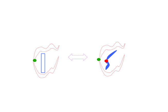
Figure 5: To Illustrate schematically how we identify a quantum entity (a particle with its wing—the wave) with the grating in double-slit experiment.

The aforementioned transverse field, on one hand acts as a biprism of focusing the wave to produce interference. On the other hand if we assume the transverse field is induced by a source, then we note that in formalism it provides another charge $\,q^{\prime}$. So in the eq. (6) of Tono there appears $qq^{\prime}$, which already exists in our formulae. This observation suggests that the use of the transverse field in experiments is consistent with our self-action assumption. Hence to some extent transverse field also models the self-action. Now let’s explain how a true micro-process of matter-wave interference happens. As for an appropriately arranged scattering processes, such as an electron scattering off a proton in atomic nucleus, the electron’s wavelength could be of the order of magnitude of the scale of proton’s radius, so that the proton simultaneously acts as an grating of electron. While the electron heads on to the proton, its wave will surround the grating (proton) and interact with itself [fig. 5]. This self-action is manifested by coupling strength $qq^{\prime}$. However, this true interference and self-action cannot be observed directly by our apparatus because of the very small scale. The true interfering procedure seems more like a gedanken experiment. We hope future studies could give clues to directly observe the effect of the true interference from scattering experiments.

Now we explain how we reference the experiments and obtain the estimation of the coupling strength $qq^{\prime}$ in perturbative limit. In experiments Tono , about $V_{\text{T}}=10~{}Volt$ transverse potential difference is used to change the directions of two wavelets, and produces a transverse momentum $k_{\text{T}}$ responsible for deriving the interference fringe (Here we omit the mechanism for deriving relationship between $V_{\text{T}}$ and $k_{\text{T}}$: $k_{\text{T}}\propto\frac{V_{\text{T}}}{\upsilon_{\text{L}}}$, $\upsilon_{\text{L}}$ is the longitudinal velocity of the electron. For more details please refer to equations in Tono ). Corresponding to the $k_{\text{T}}$ the transverse wavelength is $\lambda_{\text{T}}=\frac{2\pi}{k_{\text{T}}}\sim 500\stackrel{{\scriptstyle\circ}}{{A}}$. We are not concerned about the longitudinal wave effect for it takes such small wavelength $0.05\stackrel{{\scriptstyle\circ}}{{A}}$ that approximately it has no effect on the interference, especially when we write the final wavefunction like $\psi(x,z)=e^{ik_{z}z}\,(e^{ik_{x}x}+e^{-ik_{x}x})$. In our cases, the matter wave interferes with itself and correspondingly the ”transverse field” is provided by itself. In order to compare the self-action with the above experiment value quantitatively we propose that an incident electron heading on a proton [fig. 5], with kinetic energy similar as the ground state of hydrogen. We use hydrogen ground-state as paradigm and employ the Virial theorem $2\langle T\rangle=-\langle V\rangle$ ($\langle\ \rangle$means expectation value under a state) to evaluate the electric potential difference (volt) for self-action. $E_{0}=-13.6eV$, using $\langle T\rangle_{0}+\langle V\rangle_{0}=E_{0}$ leads to $\langle T\rangle_{0}=13.6eV$ and $\langle V\rangle_{0}=-27.2~{}eV$. Subsequently, one has $\lambda_{\text{T}}=\frac{h}{p}=h/\sqrt{2mE_{k}}\stackrel{{\scriptstyle here}}{{=}}h/\sqrt{2m\langle T\rangle_{0}}\sim 3$ $\stackrel{{\scriptstyle\circ}}{{A}}$ and $\upsilon_{\text{L}}=\frac{\lambda~{}\langle T\rangle_{0}}{h}\sim 10^{-2}c$. According to the experience on describing hydrogen, the electron with such kinetic energy tends to hold itself around nucleon with average radius of the wavelength $\lambda$. In such a manner, one end of the wave can feel the other. Self-action truly happens. On such scale around the proton, the electron can provide for itself the potential energy at most $\mid\langle V\rangle_{0}\mid=27.2~{}eV$. And according to the requirement of the experiment $\lambda_{\text{T}}=\frac{2\pi}{k_{\text{T}}}$ and $k_{\text{T}}\sim\frac{V_{\text{T}}}{\upsilon_{\text{L}}}$ Ratio , we take $V_{\text{T}}\sim 20~{}Volt$ to fit $\lambda_{\text{T}}\sim$3 $\stackrel{{\scriptstyle\circ}}{{A}}$. That means if we take $q=e$, then we should take $q^{\prime}\sim 1.8\,e$ to divide $\mid\langle V\rangle_{0}\mid=27.2~{}eV$ to get $V_{\text{T}}$. We conclude that $q\ q^{\prime}$ has the order of magnitude of $1$, but not necessarily equal to 1.

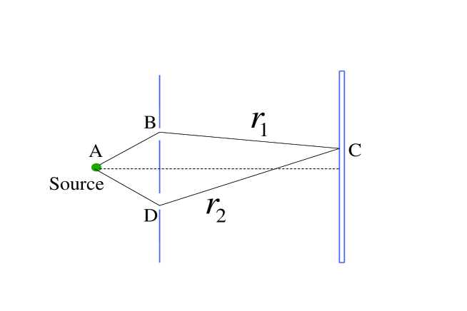
Figure 6: To show the standard explanation on double-slit experiment in quantum theory. $\triangle r=r_{1}-r_{2}$ denotes the difference of the paths from two slits to a point on screen.

VI.2 Comparison with conventional approaches and determination of $q^{\prime}$

Another way to determine the coupling strength $qq^{\prime}$ in the perturbative limit is to compare the results from eqs. (2.11), (3.12), (3.4) with standard approaches of quantum theory. We find surprisingly that $q^{\prime}$ is not a constant any longer in this way. As for the conventional/standard approaches, we note that using Feynman Path Integral Bar and using Huygens-Fresnel principle [Fig. 6] yield the same interference expression—proportional to $\cos^{2}\theta=\cos^{2}(\frac{2\pi}{\lambda}\triangle r)=\cos^{2}(\frac{p}{\hbar}\triangle r)$, where $\triangle r$ is the difference of paths from two slits to a point on screen $\triangle r=r_{1}-r_{2}$. The expression can be derived from eqs. (11) (14) and (17) of Ref. Bar . Referring to Fig. 6 we may write the difference $\triangle r$ as follows

$$\triangle r=r_{1}-r_{2}=\widehat{ABC}-\widehat{ADC}=\int_{ABC}d\mathbf{x}-\int_{ADC}d\mathbf{x}=\oint_{ABCDA}d\mathbf{x}\text{ ,}$$ (6.1)

here we use $\widehat{ABC}$ to denote a path, and the subscripts of integral signs denote the same thing. With the eq. (6.1) and $\cos^{2}(\frac{p}{\hbar}\triangle r)=\cos^{2}\theta=\mid\frac{1}{2}(e^{i\theta/2}+e^{-i\theta/2})\mid^{2}=\mid\frac{1}{2}(1+e^{i\theta})\mid^{2}$, and assuming the module of momentum $p=\mid\mathbf{p}\mid$ is approximately a constant, $\cos^{2}(\frac{p}{\hbar}\triangle r)$ can be formally written in the style of eq. (2.11), with $e^{i\theta}$ as

$$e^{i\theta}=e^{i\oint\mathbf{p}\cdot d\mathbf{x}}\text{ ,}$$ (6.2)

the loop integral is along the path $\widehat{ABCDA}$, from now on the natural unit is understood when $\hbar$ is omitted.

So far we have two ways to perform the comparison. One way is to compare eq. (3.4), $i.e.$, $e^{i\,q\oint d\mathbf{x}\cdot\mathbf{A}}$ ($q^{\prime}$ absorbed in $\mathbf{A}$) with eq. (6.2), $i.e.$, $e^{i\oint\mathbf{p}\cdot d\mathbf{x}}$. Another way is to compare $\cos^{2}(qq^{\prime}2\pi k_{i})$ [derived from (2.11), (3.12)] with $\cos^{2}(\frac{p}{\hbar}\triangle r)$. Obviously the two ways are identified. If we take the former way, then we go back to eq. (5.7) with another obvious form

$$e^{i\oint(\mathbf{p}-q\mathbf{A})\cdot d\mathbf{x}}=1\text{ .}$$ (6.3)

Eqs. (6.3),(5.7) show the consistency of our previous arguments— the lack of kinetic part in the Action form of eq. (2.11) yields the equivalence of our approach and conventional approaches in perturbative case. However we cannot directly extract the value of $qq^{\prime}$ from eq. (6.3). On the other hand, if we take the latter way, then the straightforward conclusion is that the value $q\/q^{\prime}$ depends on $\frac{\triangle r}{\lambda}$, since $\frac{p}{\hbar}\triangle r=\frac{2\pi}{\lambda}\triangle r$. This indicates that if the incident momentum (thus $\lambda$) is given and $q=e=1$, then $q^{\prime}$ is not a constant but varies with $\triangle r$. For example, for the first maximum when $\theta=2\pi$ and $\triangle r=r_{1}-r_{2}=\lambda$, from eq. (6.3) and $\cos^{2}(\frac{p}{\hbar}\triangle r)=\cos^{2}(qq^{\prime}2\pi k_{i})$ we can infer the value $A=\frac{h}{\triangle r}=p$, in such cases $A$ gets the full value of $p$ , correspondingly $q^{\prime}=1$ (Here $q^{\prime}$ is just the ratio of modules $A=\mid\mathbf{A}\mid$ and $p=\mid\mathbf{p}\mid$, not involved their vector characteristic.). Mostly the value of $A$ is just a part of $p$. In this sense, the corresponding strength of $\mathbf{A}$, i.e., $q^{\prime}$, has its value in the interval $[0,1]$. Obviously the self-action $A_{\mu}$ is path-dependent and not a conservative potential. The path-dependence stems from the attempt to describe $A_{\mu}$—which is intrinsically nonlocal—by using point-wise (particle) method. $A_{\mu}$ only shows its definite properties in nonlocal phenomenon when global measurements are performed. In any local detection $A_{\mu}$ may display its uncertainty, and here the value of $\mathbf{A}$ varies with the paths’ direction.

Now one may wonder what the relationship of the above self-action $A_{\mu}$ and momentum $p_{\mu}$ is. Our explanation is that for (self-)interaction $A_{\mu}$, in Dirac equation $(\not p-\not A)\psi=m\psi$ or in Schrödinger equation $i\hbar\frac{\partial\psi}{\partial t}=[\frac{(\mathbf{p}-\mathbf{A})^{2}}{2m}+V(\vec{r})]\psi$ (with charge $q^{\prime}$ already absorbed in $\not A$ or $\mathbf{A}$), $p^{\mu}$ and $A^{\mu}$ ($\mathbf{p}$ and $\mathbf{A}$) are on the same foot. $A_{\mu}$ can be born from $p_{\mu}$, and vice versa (This statement is to some extent implied by the aforementioned characteristic of the self-action, eq. (3.5) $A^{\mu}\sim j^{\mu}$). Since $\mathbf{A}$ is a vector, to speak $A$ as a part of $p$ may induce confusion, for example possibly $\mid\mathbf{p-A}\mid>\mid\mathbf{p}\mid$. Whereas on the other hand, eq. (6.3) can reduce the complexity by just performing an integral. As for the coupling strength $q^{\prime}$ we don’t consider such complexity and just use the results after the line integral has been performed. At least this statement pertains the quantum interference. In Introduction we have asserted that the wave of quantum entity can be viewed as its wing. Now we may question what is on earth in the wing (to speak equally, in the wave). Through the above analysis, we now have confidence to conclude: in the wing, it is just the self-action potential $A_{\mu}$, or the momentum $p_{\mu}$, or their mixture. When interactions/observations occur, $A_{\mu}$ is responsible for interfering (interacting) with itself and exhibiting its wave aspect, while $p_{\mu}$ plays the role of ”flying” and defining paths of the particle. They transfer to each other constantly and may not be separated physically. This picture deserves further study.

For the nonperturbative limit, we have eq. (5.16): $\det\not A=0$, which corresponds to $\frac{1}{N}\int[D\bar{\psi}][D\psi]e^{i\int\bar{\psi}\not A\psi d^{4}x}=0$ and thus $e^{i\int\bar{\psi}\not A\psi d^{4}x}=0$ for quantum interference. If assuming the eq. (3.12) is also available to nonperturbative cases, we conclude that only when $q^{\prime}q=-\infty$ does $\det\not A=0$ hold. This indicates that if $q=e=1$ then $q^{\prime}$ takes the value $\infty$, consistent with the word ”nonperturbative”. Thus far we have certified the conclusions from eqs. (2.9), (3.12) and (5.16) and ref. Wanng are consistent for nonperturbative limit.

VII Summary and Remarks

Throughout this whole paper we are pursuing a new understanding of quantum interference based on the perspective of matter wave’s self-action. By the special formalism of the interference we find out that the interference pattern has the common form of being the superposition of Cosine functions, in accordance with the experimental results from single electrons. By comparing the phase factors induced by Schrödinger current and Dirac current, it follows that the fermions with and without a large magnetic moment would give rise to different interference fringes due to a tiny spin-current effect, which awaits for test by experiment. By analyzing the general formalism of the interference, we predict that there is no interference phenomenon when the self-action is nonperturbative. In particular, we understand that the self-action $A_{\mu}$ can be born from momentum $p_{\mu}$ by comparing the general formalism in perturbative limit with conventional approaches of quantum theory. The strength of self-action is found to fall in the interval $[0,1]$ by such comparisons.

A novel aspect of this paper is the formalism we have followed. From the metric form $G(\bar{\psi},\psi)$ and its physical meaning—associated with the infinitesimally nonlocal evolution of the wave state, we can derive the formalism analogous to Feynman path-integral to interpret the interference contrast (for this analogy we have borrowed some treating methods from CQFT whenever possible). However we note from the relation $G(\bar{\psi},\psi)\sim e^{iS_{I}}$ that it is not the true Feynman path integral since the explicit form of $S_{I}$ is not the true Action. And the operators’ form $j^{\mu}A_{\mu}$ in $S_{I}$ is more like the Hamiltonian for $S-$matrix. So the understanding of this phase factor $e^{iS_{I}}$ becomes in a dilemma from the perspective of CQFT. On one hand if we view it as Feynman path integral, $S_{I}$ lacks a kinetic integral $S_{\text{k}}=\int\bar{\psi}(i\not\partial-m)\psi\/d^{4}x\sim\int\frac{\vec{p}^{2}}{2m}\/dt$. On the other hand if we regard it as the $S-$matrix in scattering, it lacks the legs to define its external propagators  Ryder .

The above discrepancy—lacking a kinetic term—originates from the difference of the geometric method we have employed and the Lagrangian method the CQFT used. In differential geometry, by construction it is not concerned about the motion of the points (point in real space or complex space), but about how the space (or the manifold) is curved. Once the curvature is defined and fixed by $R=0$, the motion of the point (to speak physically, the particle) is totally determined by the geodesic equation. Similar arguments apply equally to General Relativity. Whereas in the Lagrangian method, it works in a way of balancing the kinetic energy and the interaction potential by $\delta\mathscr{L}=0$. So the kinetic energy has to be present in Lagrangian. In our theoretical frame, the discussions are dominated by the properties of space, say, the wave-function $\psi$—space. Whereas in CQFT, the discussions are dominated by the properties of operators. In CQFT there are quantization processes (producing operators), which is irrelevant in our theory. Summarizing from Sec.V and Sec.VI we note that that discrepancy not only lays no obstacle for us to discuss physics, but also drives us farther in obtaining the strength of self-action.

Future researches along this line fall into five respects: Firstly we may extend present results to multi-slit and many-body systems. Secondly some other kinds of important self-action should also be examined, for instance, the axil vector form $\gamma_{\mu}\gamma_{5}$. Thirdly, so far the interference phenomenon in crossover regime between perturbation and nonperturbation remains unknown in the frame of GN. In addition, we may apply the physical picture or even the conclusions to scattering cases if we make in mind the grating between slits shrink to a quantum entity as shown in Fig.5. Finally, the self-action itself also deserves further investigation.

References

- (1) Claus Jönsson, Am. J. Phys., 42, 4 (1974): translated from Z. Phys. 161, 454(1961).
- (2) A. Tonomura, J. Endo, T. Matsuda, T. Kawasaki, and H. Ezawa, Am. J. Phys., 57, 117 (1989); and eqs. (2), (3), (5) for citing in sec. VI.
- (3) http://physicsworld.com/cws/article/print/9745, and references there in.
- (4) A. Zeilinger et al., Rev. Mod. Phys. 60, 1067 (1988).
- (5) Jeff Tollaksen, Yakir Aharonov, Aharon Casher, Tirzah Kaufherr and Shmuel Nussinov, New J. Phys. 12 (2010) 013023.
- (6) Olaf Nairz, Markus Arndt, and Anton Zeilinger, Am. J. Phys. 71, 319 (2003)
- (7) Hai-Jun Wang, J. Math. Phys. 49, 033513 (2008).
- (8) Sandu Popescu, Nature Physics, 6, 151 (2010).
- (9) Hai-Jun Wang, Hui Yang, Jun-Chen Su, Phys. Rev. C 68, 055204(2003): eq. (21) for Sec.II; eq. (4) for Sec.IV.
- (10) Feynman R, Quantum mechanics and path integrals, McGraw-Hill, Inc.: p29, pp.47-51.
- (11) G. Glionnaa, A.H. Blina, B. Hillera, M.C. Nemes, Marcos Sampaioa, and A.F.R. de Toledo Pizaa, Physica A 387, 1485(2008).
- (12) A. O. Barut and S. Basri, Am. J. Phys., 60, 896 (1992): eqs. (11), (14).
- (13) R. Feynman and L. Gell-Mann, Phys. Rev. 109, 193(1958).
- (14) Hai-Jun Wang, Topological current and its application in quantum mechanics, M. S. Thesis block (Lanzhou University, 1997), unpublished.
- (15) S.-S. Chern, W. H. Chen, and K. S. Lan, Lectures on Differential Geometry (World Scientific, Singapore, 1999): pp.168-170.
- (16) M. E. Peskin and D.V.Schroeder, Quantum Field Theory, Addison-Wesley Publishing Company, 1995. See pp. 50-51 for conserved current; see for instance eq.(9.24), (9.69) for integration result.
- (17) Y. Aharonov and A. Casher, Phys. Rev. Lett. 53, 319(1984).
- (18) Y. Aharonov and D. Bohm, Phys. Rev. 115, 485(1959).
- (19) A. Cimmino, G. I. Opat, A. G. Klein, H. Kaiser, S. A. Werner, M. Arif, and R. Clothier, Phys. Rev. Lett. 63, 380(1989).
- (20) A. Tonomura, N. Osakabe, T. Matsuda, T. Kawasaki, J. Endo, S. Yano and H. Yamada, Phys. Rev. Lett. 56, 792(1986).
- (21) At the starting point of Feynman integral, the nonlocal characteristic has been partially included by equally summing over all the paths. But this is ruined by the mostly used Gaussian integral and the least phase method.
- (22) Ai-Dong Bao, Hai-Bo Yao and Shi-Shu Wu, Chinese Phys. C 33(2009)177.
- (23) Michio Kaku, Quantum Field Theory, A Modern Introduction, Oxford University Press, 1993: pp. 414-429.
- (24) Phenomenologically, we keep the ratio between and unchanged in experiment Tono and our estimation.
- (25) Lewis H Ryder, Quantum Field Theory, (Cambridge University Press, 1985, 1996): pp.161-166.