Properties of satellite galaxies in the SDSS photometric survey:
luminosities, colours and projected number density profiles.

Abstract

We analyze photometric data in SDSS-DR7 to infer statistical properties of faint satellites associated to isolated bright galaxies ($M_{r}<-20.5$) in the redshift range $0.03<z<0.1$. The mean projected radial number density profile shows an excess of companions in the photometric sample around the primaries, with approximately a power law shape that extends up to $\simeq 700$ kpc. Given this overdensity signal, a suitable background subtraction method is used to study the statistical properties of the population of bound satellites, down to magnitude $M_{r}=-14.5$, in the projected radial distance range $100<r_{p}/\rm{kpc}<3<R_{vir}>$. The maximum projected distance corresponds is in the range $470-660$ kpc for the different samples. We have also considered a colour cut consistent with the observed colours of spectroscopic satellites in nearby galaxies so that distant redshifted galaxies do not dominate the statistics. We have tested the implementation of this background subtraction procedure using a mock catalogue derived from the Millenium simulation SAM galaxy catalogue based on a $\Lambda$CDM model. We find that the method is effective in reproducing the true projected radial satellite number density profile and luminosity distributions, providing confidence in the results derived from SDSS data. We find that the spatial extent of satellite systems is larger for bright, red primaries. Also, we find a larger spatial distribution of blue satellites. For the different samples analyzed, we derive the average number of satellites and their luminosity distributions down to $M_{r}=-14.5$. The mean number of satellites depends very strongly on host luminosity. Bright primaries ($M_{r}<-21.5$) host on average $\sim 6$ satellites with $M_{r}<-14.5$. This number is reduced for primaries with lower luminosities ($-21.5<M_{r}<-20.5$) which have less than $1$ satellites per host. We provide Schechter function fits to the luminosity distributions of satellite galaxies where the resulting faint end slopes equal to $−1.3\pm 0.2$, consistent with the universal value. This shows that satellites of bright primaries lack an excess population of faint objects, in agreement with the results in the Milky Way and nearby galaxies.

1. Introduction

According to the currently accepted model of structure formation, galaxy systems arise as the result of hierarchical clustering (White & Frenk, 1991; Bertschinger, 1994; Cole et al., 1994). The details by which galaxies form and evolve in dense or moderately dense environments, where galaxy-galaxy interactions are frequent and matter distributes in a rich substructure, depend on the characteristics of those environments. The assembly of galaxy systems entail the process of matter accretion, governed by gravity, as well as astrophysical phenomena, such as the efficiency of gas to cool and collapse or the energy feedback related to the late stages of stellar evolution (Viola et al., 2008; Kang et al., 2006). Some of these details are not yet fully understood, and observational evidence is fundamental to constraint structure formation and evolution models, specially because faint galaxies are more sensitive to astrophysical processes like supernova feedback and ram pressure stripping. In particular, statistical studies of systems of galaxies are key to understand the transformations of galaxies due to the interactions between galaxies and their environment (Nichol et al., 2003).

Although the formation of a galaxy is believed to take place on the potential well of a dark matter halo, not all haloes host a galaxy. As pointed out first by Klypin et al. (1999), the number of halos in numerical simulations were an order of magnitude greater than the observed number of satellites in the local group (Moore et al., 1999; Kravtsov et al., 2004; Strigari et al., 2007). This difference has been a matter of lively debate, being attributed either to a lack of observed galaxies or to an excess of formed objects in simulations. Willman et al. (2002) discussed the possibility of under counting satellite galaxies in the Milky Way and estimated the actual number of satellites in about twice the known population at that time. The authors argued that galactic extinction and stellar foreground can lead up to 33 per cent of incompleteness, and then the number of Milky Way satellites at low galactic latitude and at galacto–centric distance might be underestimated. Simon & Geha (2007) found that the number of satellites in the Milky Way system was greater than previously expected, based on an analysis of the SDSS data. With these findings, the discrepancy between the number of observed and simulated satellites reduces to a factor of nearly 4. Nevertheless, applying a background subtraction technique on photometric data from SDSS-DR7, Liu et al. (2010) found recently that the Milky Way galaxy has significantly more bright satellites than a typical galaxy of its luminosity.

The study of the spatial distribution of satellites around primaries and clusters has become favored by increasingly large galaxy redshift surveys. Many works address observational studies of radial distribution of galaxies in spectroscopic samples (Coil et al., 2006; Lin et al., 2004; Yang et al., 2005; Collister & Lahav, 2005), mostly around galaxy clusters, and on bright primary galaxies (Sales & Lambas, 2005; Chen et al., 2006). Deeper samples have been also used to compute projected density profiles, using background subtraction (Hansen et al., 2005) around MaxBCG galaxy systems. Moreover, galaxy projected density profiles were computed based on projected correlation function determinations in redshift galaxy catalogues (Li et al., 2007) and deeper photometric samples (Wang et al., 2010) around a set of spectroscopically identified galaxies.

The distribution of satellite luminosities is also key to the development of models and understanding of the processes of galaxy formation (Benson et al., 2003; Benson, 2010; Okamoto et al., 2010). Given the low luminosity of most satellites, however, their observation is usually onerous and hardly accessible outward of the Local Group. Mateo (1998) put forward a detailed census of dwarf galaxies, from which a flat faint end of the luminosity function in the Local Group could not be discarded. Background subtraction methods have been widely used to obtain galaxy luminosity function in clusters, and also results of this procedure on individual clusters have been reported (e.g. Oemler, 1974). Since it is not limited to the computation of luminosities, it can be also used to obtain the color-magnitude relation (Pimbblet, 2008). Andreon et al. (2005) present a variation of the background decontamination method, avoiding the use of arbitrary binning and incorporating the background noise as part of a refined model for the description of data. Koposov et al. (2008) presented a search methodology for Milky Way satellite galaxies in SDSS data through the computation of efficiency maps. Search for stellar concentrations using these maps suggest a luminosity distribution that steadily rises following a power law up to $M_{v}\simeq 5$. From there on, a flat distribution could not be discarded (Koposov et al., 2008).

Tollerud et al. (2008) use completeness limits for the SDSS-DR5 to implement a correction for luminosity bias. Although a first order correction would produce an increase in the faint end of the luminosity function, the authors bring forward that this result is not well enough constrained given available data. Trentham & Tully (2002) study the faint end of the galaxy luminosity function in five different local environments, from the Virgo cluster to NGC 1023 group. The authors derive an averaged luminosity distribution in the range $-18.<M_{r}<-10$ (Cousins R magnitude) and infer a faint end slope $\alpha\sim-1.2$. In the particular case of NGC 1023, a more detailed study confirmed later that the faint end is consistent with a shallow slope (Trentham & Tully, 2009). Tully & Trentham (2008) studied the NGC 5353 group and attributed a faint end slope $\alpha=-1.15$ to the fact that this group is at an intermediate evolutionary age.

Membership of individual galaxies through spectroscopic measurements is inefficient in terms of observing time, given the large fraction of background objects that have to be rejected. This results in few systems with derived luminosity function complete down to faint magnitudes. For this reason, a background subtraction technique is an efficient method to study, on a statistical basis, properties of the population of companion objects. Using deep mock catalogues constructed from a numerical simulation, Valotto et al. (2001) analyze systematic effects in the determination of the galaxy luminosity function in clusters. Their results indicate a strong tendency to derive a rising faint end when clusters are selected without redshift information. This is due to projection effects, since many of the clusters selected in 2D have no significant counterpart in 3D. Muñoz et al. (2009) use Mock catalogues constructed using GALFORM (Baugh, 2006) semianalytic model of galaxy formation to study the reliability of the statistical background subtraction method to recover the underlying observer-frame luminosity function of high redshift ($z\simeq 1$) cluster galaxies in the K_s band. These authors find that the optimal response of the method in recovering the underlying galaxy luminosity function occurs when background corrected counts of faint galaxies are complemented with photometric redshifts of bright galaxies. They also show that the increase in the number of galaxy clusters that contribute to the computations dramatically reduce stochastic errors. Christlein (2000) study luminosity functions for galaxies in loose groups and suggests that the ratio of dwarf to giant galaxies is continuously increasing from low to high mass groups. This is based on data from the Las Campanas Redshift Survey, where environment is estimated using the line-of-sight velocity dispersion of the host groups. Background subtraction has been applied to single clusters (Andreon et al., 2005; Barkhouse et al., 2007) and to ensembles of clusters (González et al., 2006).

Figure 1.— Properties of primary galaxies in the total sample. This sample comprises $51710$ galaxies brighter than $M_{r}=-20.5$ in the redshift range $0.03$ to $0.1$, satisfying the isolation criteria stated in Section 2.1.

The goal of this work is to obtain statistical properties of satellite galaxies in the magnitude range $-18.5<M_{r}<-14.5$, using SDSS photometric data. Previous studies of galaxy satellites concern mostly Milky Way and nearby galaxies, so that this work complements with a study of projected radial number density profiles, luminosity, and colour distributions for a statistically large sample of primaries within $z=0.1$. The definitions of host samples and the adopted satellite selection criteria are presented in Section 2. The details of the background subtraction procedure are given in Section 3. Then, in Section 4 we present the derived distributions of satellite properties. In order to validate the implemented method, we test it in Section 5. Finally, the main conclusions are provided in Section 6.

2. Photometric and spectroscopic data

	primaries			galaxies
sample	luminosity	colour	$N_{p}$	$R_{max}$ [kpc]	colour
S0-A-a	M${}_{r}<$-20.5	all	51710	$<$ 480	$-0.4<g-r<1.0$
S0-A-r	M${}_{r}<$-20.5	$g-r>1.0$	51710	$<$ 480	$0.4<g-r<1.0$
S0-A-b	M${}_{r}<$-20.5	$g-r<1.0$	51710	$<$ 480	$-0.4<g-r<0.4$
S1-A-a	-21.5$<M_{r}<$-20.5	all	42335	$<$ 470	$-0.4<g-r<1.0$
S1-A-r	-21.5$<M_{r}<$-20.5	$g-r>1.0$	42335	$<$ 470	$0.4<g-r<1.0$
S1-A-b	-21.5$<M_{r}<$-20.5	$g-r<1.0$	42335	$<$ 470	$-0.4<g-r<0.4$
S2-A-a	M${}_{r}<$ -21.5	all	9375	$<$ 660	$-0.4<g-r<1.0$
S2-A-r	M${}_{r}<$ -21.5	all	9375	$<$ 660	$0.4<g-r<1.0$
S2-A-b	M${}_{r}<$ -21.5	all	9375	$<$ 660	$-0.4<g-r<0.4$
S2-R-a	M${}_{r}<$ -21.5	$g-r>1.0$	4740	$<$ 660	$-0.4<g-r<1.0$
S2-R-r	M${}_{r}<$ -21.5	$g-r>1.0$	4740	$<$ 660	$0.4<g-r<1.0$
S2-R-b	M${}_{r}<$ -21.5	$g-r>1.0$	4740	$<$ 660	$-0.4<g-r<0.4$
S2-B-a	M${}_{r}<$ -21.5	$g-r<1.0$	4635	$<$ 660	$-0.4<g-r<1.0$
S2-B-r	M${}_{r}<$ -21.5	$g-r<1.0$	4635	$<$ 660	$0.4<g-r<1.0$
S2-B-b	M${}_{r}<$ -21.5	$g-r<1.0$	4635	$<$ 660	$-0.4<g-r<0.4$

Table 1Definition of satellite samples considering colour range, maximum projected distance to the primary and primary properties. The number of primaries $N_{p}$ of each sample is also indicated. Satellite galaxies have a lower bound of $g-r=-0.4$ for samples a and b. Upper case letters A, B and R stand for All, Blue and Red, respectively. Similarly, lower case letters indicate the ranges of satellite colours.

We use the large database provided by the Sloan collaboration (SDSS, Stoughton et al., 2002), which provides photometric information of objects down to faint magnitudes. This survey has been carried out using a dedicated $2.5$m telescope (Gunn et al., 2006), and comprises digital photometric information of stars and galaxies in $5$ bands (Fukugita et al., 1996; Smith et al., 2002) reduced by an automated pipeline (Lupton et al., 2001). The limiting magnitude is $22.2$ in the r–band. A set of the brightest and more concentrated galaxies in the main galaxy sample has been selected for spectroscopic follow up (Blanton et al., 2003a). This leads to the spectroscopic galaxy catalogue, which contains galaxies with Petrosian magnitude $r<17.77$ (Strauss et al., 2002). Both photometric and spectroscopic data are accessible through a web interface to the public releases of the survey. The Data Release 7 comprises nearly 18 Tb of catalogued data for objects identified as galaxies by the automated data reduction pipeline (Data Release 7, Abazajian et al., 2009). The main galaxy sample comprises $691055$ galaxies with 95 per cent completeness down to a limiting magnitude $r_{lim}=17.77$ in the $r$-band. The surface brightness limits are imposed by the instrument capabilities and the automated reduction pipeline, so that these data sets allow to retrieve information about galaxies above the surface brightness limit of the catalogue, $\mu_{50}\leq 24.5\;mag\;arcsec^{-2}$ in the Petrosian r-band (Strauss et al., 2002). All galaxies in this sample have redshift measurements and serve in this work as primary targets for the study of fainter galaxies, accessed from a deeper photometric sample. We obtain statistical properties of faint satellites, most of them not present in the spectroscopic survey, associated to primaries with measured redshifts in the range 0.03 to 0.1 To this aim, we use the New York Value Added Galaxy Catalog (NYU-VAGC, Blanton et al., 2005) to extract photometric information of neighboring galaxies of primaries. This catalogue is based on the sixth release of the Sloan Digital Sky Survey, and covers $9583$ deg² of sky distributed into a northern cap and three southern stripes. We notice that the sky coverage of the main galaxy sample in DR7 is approximately included in the NYU-VAGC DR6 area, so that the cross-correlation between these two catalogues is suitable for the purpose of this work. We used software HEALPix (Górski et al., 2005) to optimize the data processing of the galaxy catalogues.

2.1. Host samples and galaxy selection criteria

We have considered primaries brighter than $M_{p}=-20.5$ ($r$–band luminosities) in the redshift range $0.03$ to $0.1$, applying an isolation criterion in order to avoid high density environments such as pairs or groups of galaxies. The density contrast around galaxies fainter than $M_{p}=-20.5$ is low and comparable to Poisson uncertainty. Since the method, detailed in Section 3, is based on the presence of a strong signal to background, we left them out of consideration in defining the samples of hosts. These primaries are constrained to have no neighbors brighter than $M_{p}+2$ within projected distance $700$ kpc and relative radial velocity difference $700$ km/s. These criteria are similar to those adopted in previous studies using spectroscopic samples (Sales & Lambas, 2005; Chen et al., 2006; Agustsson & Brainerd, 2010), and are intended to select and isolate halos where a dominating, assumed central galaxy of the satellite system is found. The total sample of primaries comprises $51710$ objects brighter than $M_{p}=-20.5$ in the redshift range $0.03$ to $0.1$.

Taking into account galaxy luminosities and colours, we have considered different subsamples of primaries in order to explore possible dependencies of the satellite properties as a function of host properties. The description of the subsamples considered is given in Table 1. Subsample names are indexed on a three character basis: a number indicating the host luminosity selection (”0” for full sample, ”1” for hosts with $-21.5<M_{r}<-20.5$, and ”2” for hosts with $M_{r}<-21.5$); and two letters indicating host and satellite colours. For simplicity, uppercase characters correspond to primary galaxy colours (A,R,B: All, Red, Blue), while lowercase indicate satellite colours (a, r, b standing for all, red and blue respectively). In Fig. 1 we show the distributions of $r$–band absolute magnitudes, $g-r$ colours and redshifts of hosts in the total sample. The bimodal distribution of primary galaxy colours can be clearly appreciated, and we use a colour cut $g-r$=0.8 to separate subsamples according to host colour.

3. Background subtraction method

The background subtraction methodology are based on the simple idea of counting the number of objects in a region where a given signal is expected to lie, superposed to an uncorrelated noise, and subtracting a statistical estimation of that noise. In this case, the signal is due to the presence of satellite galaxies in systems dominated by a central and luminous galaxy, and the noise is associated to the background and foreground galaxies not dynamically linked to the primary galaxy. Then, it allows to statistically obtain properties of the faint galaxies associated to the primaries, without the need of redshift information for individual objects. This is accomplished provided that the working hypothesis of the central primary is satisfied, and convenient ranges of observed parameters are chosen, so that to minimize the contribution of background counts. Although the method does not allow to quantify the contribution to the signal of each individual object, it is possible to obtain statistical estimates of probability density distributions describing galaxy properties. This is accomplished by restricting galaxies to a fixed bin of the variable, for instance the luminosity of the satellite or their distance to the central galaxy, and normalizing to the number of contributing systems in that bin, after implementing the background subtraction.

Within the hierarchical clustering paradigm, the matter distribution can be roughly described by a set of halos populated with galaxies, according to certain recipes that depend on galaxy type (Cooray & Sheth, 2002). This model can give insight to adopt an appropriate choice of the centers, which is key to increase the signal from the satellite population against the background noise and obtain reliable results using this method. Central galaxies play a different role than the rest of objects within the halo due to its particular accretion history, related to the merging of massive galaxies in each halo, and eventually the accretion of most of the available gas and even other minor galaxies (Cooray & Milosavljevic, 2005). While galactic cannibalism has been proposed as the main mechanism for building up central galaxies (Ostriker & Tremaine, 1975; White, 1976; Vale & Ostriker, 2006), it has also been suggested that major mergers (Lin et al., 2004) and dry mergers (Liu et al., 2009; Khochfar & Silk, 2009) play an important role in the different stages of their evolution. From a dynamic point of view, relative velocities of central galaxies with respect to the halos in which they reside are very small, compared to the large velocity dispersion of satellite galaxies. This leads to a clear observational distinction between central and satellite galaxies (Vale & Ostriker, 2006). It is also known that a central galaxy is often the most luminous galaxy within their halo (Vale & Ostriker, 2006). Even when this ”central galaxy paradigm” has been claimed to be inaccurate (Skibba et al., 2010), specially in high mass systems, the precise location of the center of the halo is not crucial for the implementation of the method, since it integrates galaxy counts in a region where overdensity signal is clearly present. Still, the location of the brightest galaxy in this special type of galaxy systems, where a galaxy strongly dominates in luminosity and the total mass of the systems is quite low, is a very good approximation to the position of the center of the galaxy system. Under these assumptions, the brightest galaxies are expected to reside in the centers of haloes (Jones & Forman, 1984; Lin et al., 2004; Smith et al., 2005), and can be used statistically to analyze galaxy overdensities associated to satellites. Accordingly, we limit the sample of centers to bright isolated galaxies, since they are likely central galaxies of small haloes.

Figure 2.— Colour distributions of faint galaxies with measured redshifts in SDSS, in three different absolute magnitude intervals. Curves show spline interpolation.

Figure 3.— Colour distributions of excess counts of companions, in three different magnitude intervals, of bright primaries (sample S2-A) resulting from a background subtraction calculation.

3.1. Constraints imposed by the data

The main requirement for the success of a statistical background subtraction method relies on a significant mean overdensity around a given sample of primaries. This fact leaded us to consider bright galaxies, $M_{p}<-20.5$, since the neighborhood of fainter primaries do not show a significant density enhancement in SDSS data. The uncertainty of the background decontamination procedure is dominated by Poissonian statistics of subtraction of large numbers. A significant increase in the signal to noise ratio of satellites can be achieved by eliminating those galaxies with a low probability of association to the primaries. To this end, we restrict the parameter space of galaxies in the photometric catalogue so that we only use ranges of those parameters where the hypothesis assumed in the background subtraction method are best satisfied, and reliable estimations of luminosity, colour and projected radial distributions can be obtained. We impose constraints on apparent magnitude, colours and radial distance of photometric galaxies. Accordingly, we adopted $M_{r}<-14.$, $-0.4<g-r<1.0$, and a projected radial distance in the range $100$ kpc to $3<R_{vir}>$, which we discuss in detail in what follows.

The redshift range of primaries determines, along with the limiting magnitude of the photometric sample, the maximum luminosity that can be studied. Given the limiting magnitude of $21.5$ in the r–band, and a minimum redshift for the primaries of $0.03$, we chose the maximum luminosity $M_{r}-5log(h)\sim-14$ in the r–band. The limiting magnitude we use is lesser than the limiting magnitude from SDSS in order to ensure 100 per cent completeness (Abazajian et al., 2004).

We show in Fig. 2 the observed colour distributions of SDSS satellite galaxies derived from the spectroscopic sample in three different absolute magnitude bins between $-18.5$ and $-14.5$. It can be appreciated in this figure that a colour cut in $g-r<1$ includes most of faint companion objects, and has the advantage of removing high redshift galaxies reddened by K-correction. Therefore, in all computations we exclude objects redder than this threshold to lower the noise due to the presence of high redshift galaxies. A clear indication that our colour cut $g-r=1$ is a suitable threshold to remove high redshift galaxies can be seen by inspection to Fig. 3 where we have applied background subtraction counts to sample S2-A in the range $100$ kpc$<r_{p}<660$ kpc. The observed lack of excess signal beyond $g-r=1$ shows that our method is effective in detecting companion galaxies in the colour range $-0.4<g-r<1$. This is also a convenient cut according to determinations of satellite colours in semianalytic models of galaxy formation (Font et al., 2008) and galaxies in groups in SDSS-DR2 data (Weinmann et al., 2006). We have applied the same colour cut $g-r<1$ to galaxies in the mock catalogue, as described in Section 5.

In Fig. 4 we show the projected density profile of galaxies, in the selected color range $-0.4<g-r<1.0$, around primaries of sample S2-A-a. For comparison, we also show the corresponding of galaxies with $g-r>1$. As can be appreciated, a significant excess of $-0.4<g-r<1.0$ galaxies is observed beyond $100$ kpc, while red galaxies, $g-r>1.0$ (mainly consisting in strongly redshifted background galaxies) show a null flat profile consistent with a uniform radial distribution (shaded region in Fig. 4), which also gives support to our choice for the colour range of satellites. However, as can be appreciated in the inset of Fig. 4, we notice that the projected density profile of red galaxies is not uniform in the inmost region around the luminous primary galaxies. This shows that the hypothesis of a uniform background fails within $100$ kpc for this data set. Hence, in the computation of the statistical distributions, namely luminosity and colours, galaxies are restricted to be at a projected radial distance of at least $100$ kpc. This radial distance is consistent with previous findings that indicate the presence of an extended stellar halo associated to luminous galaxies. This issue could lead to a failure of SDSS automated pipeline in the detection of low surface brightness galaxies, either satellites or foreground/background galaxies. Nierenberg et al. (2011) study the spatial distribution of faint satellites at intermediate redshifts ($0.1<z<0.8$) using high resolution HST images of early type galaxies taken from GOODS fields. The authors model the light profile of host galaxies in order to study the population of faint satellites. This model gives the spatial distribution of satellites near the primaries as a combination of a satellite population with a power law radial profile superimposed to an isotropic and homogeneous background population. The method proposed by the authors requires the analysis of images of all hosts, which is beyond the scope of this work. This stellar halo component extends up to approximately $100$ kpc, according to statistical determinations in SDSS (Zibetti et al., 2004; Bergvall et al., 2010; Tal & van Dokkum, 2011).

Figure 4.— Mean projected density profile of galaxies with $g-r<1.0$ around primaries with $M_{r}<-21.5$ (sample S2). Shaded region show the projected density profile of red galaxies around the same primaries with $g-r>1.0$ (mainly background objects), within 1-$\sigma$ uncertainties.

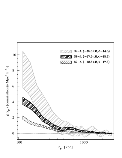
Figure 5.— Density profile of satellites in S2-A sample selected by satellite luminosity. Galaxies are selected in the colour range $-0.4<g-r<1.0$. Fainter satellites show a steeper and more concentrated density profile. Brighter satellites show a greater spatial extension, but smaller excess.

An additional problem is related to fluctuations of luminosity density the extended images of luminous galaxies, for example in the external parts of large, late-type galaxies at low redshift. Since SDSS images are analyzed to identify galaxies by automatic algorithms, luminosity concentrations (which are part of the primary) are often confused and classified as many faint fake galaxies. This problem is hard to address, and is part of proposed SDSS ”research challenges” . The deblending process resulting from the current SDSS-DR7 pipeline appears to induce an artificial neighbor excess, which strongly difficults the treatment of data on regions close to the primary (see e.g. Tollerud et al. (2011)), specially in late-type galaxies where rich luminosity patterns are present on the disk. We also show in the inset of Fig. 4 the mean value of the $R_{90}$ distribution of primaries in sample S2, indicated with an arrow. Also, Brainerd (2005) argue that satellites show a strong preference for being aligned with the host major axis on scales below $100$ kpc, while on larger scales ($250\lesssim r_{p}/\rm{kpc}\lesssim 500$) the satellite distribution is consistent with an isotropic distribution. Due to this anisotropy, satellites close and near the major axis of the primary could be confused to luminosity enhancements of the disk of the primary when using photometric data. Both fake galaxies and depleted background are likely to coexist, and can not be directly disentangled. This might be also complicated by other effects such as dust obscuration by primary disk, alignment of satellites with disks and segregation of satellite properties with radial distance (Chen, 2008; Ann et al., 2008).

The chosen minimum distance of $100$ kpc corresponds roughly to $0.5-0.6R_{vir}$. Tollerud et al. (2011) find that 12 per cent of Milky Way-like galaxies host an LMC-like satellite within $75$ kpc projected distance, while 42 per cent lie within $250$ kpc. In the sample with the lower mean virial radius (S1) this means that, for a typical primary galaxy, and an assumed power law profile of the satellite distribution outside $20$ kpc ($\gamma=2.$, see Table 2), only about 20 per cent of satellites within $100$ kpc are not included in the analysis of sample S0 and $\sim 14$ per cent for sample S2.

The projected density profile shows an excess of galaxy counts per unit area, with respect to the local background, which decreases beyond $R_{p}\approx 500$ kpc, but depends on the sample of primaries and satellites considered. Sales & Lambas (2005) analize simulations and find that the turn around radius of satellite galaxies is of order $3\,R_{vir}$. These findings are also consistent with the approximate location of the turnaround radius according to the simple secondary infall model Bertschinger (1985). Then, in the computation of the statistical distributions, galaxies are also restricted to be at a projected radial distance from the primary of up to 3 times the mean virial radius in each sample. Using the masses of dark matter haloes hosting primary galaxies in a mock catalogue (described in Section 5), we find a variation in the distributions of virial radius of primary galaxies corresponding to samples S0, S1 and S2. While the median virial radius $<R_{vir}>$ for sample S0 is $160$ kpc, it changes to $157$ kpc for sample S1 and to $220$ kpc for sample S2. We adopt a maximum radius for each sample (S0, S1 and S2) $R_{max}=3\,<R_{vir}>$, i.e., $R_{max}=480$ kpc for sample S0, $R_{max}=470$ kpc for sample S1, and $R_{max}=660$ kpc for sample S2. These values are also consistent with the results of Chen et al. (2006) and Liu et al. (2010), who find that the fraction of interlopers remain low within $500kpc$ projected distance. In Section 5 we use a mock catalogue to test the background subtraction method, and confirm that the choice of this maximum radius is convenient to maintain a low level of contamination by foreground and background galaxies.

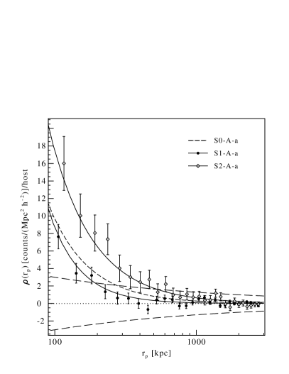
Figure 6.— Density profile of excess galaxies around primaries in samples S0-A-a, S1-A-a, and S2-A-a. For simplicity, only the power law fit is shown for sample S0-A-a, along with the uncertainty amplitude in long dashed lines.

In Fig. 5 we show the resulting profiles for different ranges in satellite luminosities, where it can be seen that fainter satellites are more strongly concentrated. This maximum projected radius $3<R_{vir}>$ is suitable to study satellite properties in the range $-18.5<M_{r}<-14.5$, although brightest satellites can be detected beyond this value. Agustsson & Brainerd (2006) analyze simulations in a LCDM framework to study the locations of satellite galaxies. The authors define their samples of satellites as all galaxies around luminous central galaxies, that have a difference in projected distance lesser than 500kpc, and a difference in radial velocity below 500-1000 km/s, according to the selected sample. Primary galaxies have a median host halo virial radius of ∼ 275 kpc. Ann et al. (2008) analyze satellite galaxies in SDSS-DR5 in order to study the dependence of radial distribution and environment of galaxy morphology. These works show agreement on the extension of the satellite populations up to $\sim 500$ kpc.

In order to account for large scale angular fluctuations in the distribution of faint galaxies we have used a local background in all samples. The density profile is approximately constant beyond $1.5$ Mpc (see Fig. 6), therefore we chose the density in the projected radius interval $2000-3000$ kpc as the reference level of background galaxy counts. Although a global background could be used instead, we argue that a mean number density of galaxies obtained locally is better suited to account for possible irregularities in the number density of background galaxies. We use the redshift of each host to compute the absolute magnitudes corresponding to the excess galaxy counts in different apparent magnitudes, by assuming that these true companion galaxies are at the same redshift than the primary. We compute a composite luminosity distribution by averaging over a sample of primaries with a given set of properties. The number counts per magnitude bin on the resulting composite luminosity distribution estimates are normalized according to the appropriate limits of magnitudes in order to assure completeness:

$$N_{i}=\sum_{j}{N_{ij}F_{j}C_{j}}$$ (1)

where $N_{i}$ is the number of galaxies within the $i$-th magnitude bin for the total ensemble, and $N_{ij}$ is the number of galaxies in that magnitude bin for the $j$-th primary. The normalization for each magnitude bin is given by the fraction of fields contributing within the completeness limits, $C_{j}$, and by the fractional area, $F_{j}$, determined by the mask.

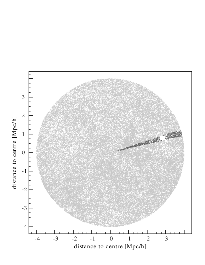
Figure 7.— In left panel we show an example of a field centered on a bright galaxy affected by a mask, where each point represents a galaxy in the photometric sample. Using the Monte Carlo procedure to construct a detailed mask, as described in Section 3.2, an angular fraction is eliminated (dark points) in the region where a hole is located. In this typical example, we use a 98.6 per cent of the area in the field. On the right panel, we show the distribution of the fraction of areas of the primary fields $F$ after application of the masks. Fields with $F<0.9$ are excluded from the analysis.

3.2. Detailed masks

Since we expect a relatively small number of satellites compared to the total background number counts, several primaries should be used in order to add up the signal over the background noise. Since the number of satellites grows approximately linearly with the number of hosts and Poisson errors scale as the square root of the number of galaxies, a large number of fields is required in order to override the satellite population number over the background counts. In Table 1 it can be seen that all samples comprise thousands of primaries, and in particular, the smallest sample (S2-B) contains nearly $5000$ host galaxies. Fields of galaxies are extracted from the NYU-VAGC around the primary galaxies. The survey area from which the data is drawn has not, however, a simple geometry, and the detailed structure of holes and borders is an additional problem for the method used in this work. While the external borders are relatively simple, the survey has small disconnected holes of a variety of shapes. The origin of these holes relies on the presence of several bright objects which blanket the background galaxies, in particular the faint ones. The most important are stars in our galaxy, but we can also mention the trails of solar system objects or artificial satellites, cosmic rays, etc. Moreover, in certain cases, there is a regular pattern of holes, sometimes associated to an incomplete structure of stripes. Therefore, a mask must be built for each of the fields, in order to correctly account for the effective areas used in the method. As an example we show in Fig. 7 a typical field where a hole in the projected distribution of galaxies can be seen. The construction of the mask is based on the ansatz that, on a coarse resolution, faint galaxies provide a dense, nearly uniform background so that the holes can be directly associated to the absence of faint objects in a patch of the sky. In order to identify regions without faint galaxies we use a Monte Carlo method. The method consists in determining distances from the faint galaxies in the photometric sample to a large number of uniformly distributed random points within the area considered. Those random points that are separated from its nearest neighbor galaxy at least by a percolation radius $r_{0}$, are used to characterize the holes, i.e., holes are detected as concentrations of random points percolated by using this criteria. We have adopted a percolation radius $r_{0}$ equal to a fraction $f$ of the mean angular galaxy separation $<D>$ of each field. The value of $f$ was obtained by diluting several realizations of complete and dense fields of galaxies, and retrieving in each case the ideal limiting value for the percolation radius. We calibrated the value of this fraction, and found a mean value of $f=0.17$, with a slight variation as a function of the projected galaxy density in each field (Lares, 2009). Given the complicated shapes of identified holes, we simply eliminate angular sectors that contain the random points inside holes, as can be appreciated in Fig. 7. In this Figure we show in grey points the locations of galaxies used in the background subtraction procedure, and in dark grey points the locations of galaxies in the same angular sector that the mask hole that were not considered in such analysis. We computed the distribution of the fractions of angular areas finally used in the analysis presented in the following sections. We show this distribution in Fig. 7, where we have indicated the location of the fraction of used area of the field shown in Fig. 7. It can be seen from Fig. 7 the high level of completeness of the data, with 90 per cent of the fields having less than 5 per cent of their areas lost by the application of the masks. Furthermore, there is a negligible amount of fields with less than 90 per cent angular completeness, so that these fields are excluded from the analysis. Notice that this method is able to identify detailed small scale features in the angular distribution of photometric galaxies. Given the resolution required to account for small holes, a mask constructed by using standard methods (e.g. Hamilton & Tegmark, 2004; Górski et al., 2005; Swanson et al., 2008) would be computationally expensive for reaching the same accuracy than the used methodology. Besides, this procedure allows to adapt the percolation radius for each field, instead of using a fixed resolution on a pixelization scheme, and makes the computation of areas straightforward by using angular bins.

4. Results: statistical properties of satellite galaxies

4.1. Determination of projected radial distributions

Although it would be desirable to consider satellites as close as possible to the primary galaxies, there are systematic detection biases that strongly limit this possibility. We have also observed that close to primaries, the detection of faint objects can be strongly biased due to several facts such as obscuration, confusion, etc. Galaxies behind bright galaxy discs could also be covered by intrinsic absorption, producing significative changes in the observed magnitudes. Taking these issues into account, we have adopted a minimum distance of $100$ kpc to primaries for our analysis assuring reliable and systematic-free samples of faint objects. We considered galaxies in projected radial distance bins from the corresponding primaries to compute the averaged density profile for the different samples. The radial bins are chosen so that all the resulting rings have the same area. This partition allows to explore the inner region with more detail. In Fig. 6 we show the density profile of samples S1-A-a and S2-A-a corresponding to all primaries with $-21.5<M_{r}<-20.5$ and $-22.0<M_{r}<-21.5$ respectively, without restrictions in the colours of primaries nor satellites. It can be appreciated the smoothly declining mean density profiles, although the extent of the overdense region is larger for the brightest hosts. We have also computed the density profiles for red ($0.4<g-r<1.0$) and blue ($g-r<0.4$) companion galaxies of bright primaries with $M_{r}<-21.5$, (samples S2-A-r and S2-A-b). It can be seen by inspection to Fig. 6 that the two profiles have a similar spatial extent and radial density profiles.

We have fitted power law functions to the radial density profiles $\rho(r_{p})=Ar_{p}^{-\gamma}$. The resulting values of the profile slope $\gamma$ are given in Table 2 where it can be seen that the companion galaxies of primaries show in general a concentrated distribution. Agustsson & Brainerd (2010) investigate the locations of the satellites of relatively isolated host galaxies in the Sloan Digital Sky Survey and the Millennium Run simulation. The authors find that the distribution of the satellites within 500kpc of red, high mass hosts with low star formation, differ from the distribution of satellites of blue, low mass hosts with low star formation.

4.2. Mean number of satellites and luminosity distributions

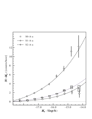
Figure 8.— Cumulative luminosity distributions of excess galaxies around primaries in the three defined samples (dubbed S0, S1 and S2). Lines represent the best Schechter function fits to the obtained distributions (see text).

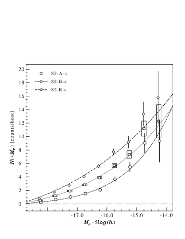
Figure 9.— Cumulative luminosity distributions of excess galaxies around bright primaries ($M_{r}<-21.5$). Luminosity distributions for red and blue hosts (with a colour cut in $g-r=1.0$) are also shown.

We compute the mean number of satellites beyond $R_{min}=100$ kpc and up to a projected radial distance equivalent to $R_{max}=3<R_{vir}>$ for each sample, no extremely red galaxies ($g-r>1$) where included, since both restrictions where applied in the computations as previously explained (Section 3.1). The mean number of satellites (shown in Table 2) $<N_{s}>$ in the magnitude range $M_{r}<-14.5$ is estimated for all primary samples, as:

$$<N_{s}>=\frac{1}{N_{p}}\sum_{j=1}^{n}N_{in}^{j}-\frac{1}{A}N_{out}^{j},$$ (2)

where $N_{p}$ is the number of primaries in the sample, $N_{in}^{j}$ is the number of galaxies inside the inner ring of the $j$-th field, and $N_{out}^{j}$ is the number of galaxies inside the chosen outer ring. The area of the background, corrected by the mask, is $A$ times the area enclosed between the chosen radius of the signal inner region. The isolation condition ensures that bright galaxies chosen as centers are somewhat separated from other luminous galaxies, and is intended for selecting a given group of galaxies with similar properties, but does not affect the calculation of the luminosity function, given that it includes satellites at most as bright as $M_{s}=M_{p}+2$ The faintest possible in sample S0 has an absolute magnitude $M_{p}=-20.5$, so that no satellites with $M_{s}<-18.5$ are expected to be found in the spectroscopic sample. If galaxies brighter than this limit are considered, the sample of satellites would not be complete, so we limit the study of satellites to the range $-18.5<r<-14.5$. We assign uncertainty estimates to the mean number of satellites using Poisson errors resulting from the number counts of galaxies within $R_{max}$ from the primaries and the expected number of background galaxies:

$$\centering\epsilon=\frac{1}{N_{p}}\sqrt{\sum_{j=1}^{n}{N_{in}^{j}}+\frac{1}{A}N_{out}^{j}}.\@add@centering$$ (3)

We find that the number of satellites depends on primary luminosity. As can be seen in Table 2, sample S1 has on typically 1 satellite within the range of color and magnitude adopted. This number increases to nearly 6 satellites on average for sample S2, equally distributed between red and blue satellites. This result is consistent with that of Macciò et al. (2010), who study numerical simulations of Milky Way sized haloes as predicted by Cold Dark Matter based models of galaxy formation and find that the number of satellite galaxies increase with halo mass. On the other hand, the number of companion objects of primaries on the same luminosity interval has not a clear dependence with satellite $g-r$ colour index. In all samples of primaries, the numbers of blue and red satellites are comparable. We notice that this is valid for the ranges of projected radius and magnitudes used in this study (Table 1).

In the computation of the luminosity distribution, a convenient normalization is set for each magnitude bin, so that the mean number of satellites per magnitude interval per primary is obtained. This was achieved by dividing the number counts of excess galaxies by the number of contributing primaries in each magnitude bin. We performed Schechter fits (Schechter, 1976) to the differential histograms of magnitude distributions, and computed the faint end slopes, given in Table 2. For samples S0-A-a, S1-A-a and S2-A-a, the luminosity distributions are consistent with a Schechter function with a faint–end slope of $-1.3\pm 0.2$, adopting a universal $M_{\star}$ value of $-20.44$ (Blanton et al., 2003b).

sample	$<N_{s}>$	$\gamma$
S0-A-a	$1.5\pm 0.4$	-2.0$\pm$0.2
S0-A-r	$0.7\pm 0.4$	-2.1$\pm$0.5
S0-A-b	$0.9\pm 0.2$	-1.8$\pm$0.4
S1-A-a	$0.9\pm 0.5$	-2.4$\pm$0.3
S1-A-r	$0.2\pm 0.5$	-2.0$\pm$2.0
S1-A-b	$0.7\pm 0.2$	-1.9$\pm$0.5
S2-A-a	$6.1\pm 1.4$	-1.5$\pm$0.4
S2-A-r	$3.4\pm 1.3$	-1.5$\pm$0.7
S2-A-b	$2.7\pm 0.6$	-1.6$\pm$0.3
S2-R-a	$7.8\pm 2.2$	-1.1$\pm$0.6
S2-R-r	$4.2\pm 2.0$	-0.8$\pm$0.7
S2-R-b	$3.7\pm 0.9$	-1.8$\pm$0.2
S2-B-a	$4.7\pm 1.8$	-1.9$\pm$0.5
S2-B-r	$2.5\pm 1.6$	-2.1$\pm$0.7
S2-B-b	$2.1\pm 1.0$	-1.5$\pm$0.6

Table 2 Mean number of satellites for each sample, and fit parameters for their background subtraction derived projected density profile. The mean number of satellites per host $<N_{s}>$ was calculated in the $r$–band. Errors are calculated as described in Section 3. In all cases, primary redshifts lie in the range $0.03<z<0.10$ and the indicated number of satellites include objects in the magnitude range $-18.5<M<-14.5$, with the $g-r$ colour index limited to the range $-0.4<g-g<1.0$, and at a projected distance between $100kpc$ and $R_{max}$ (see Table 1).

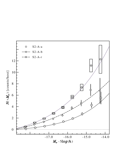
Figure 10.— Cumulative luminosity distributions of blue ($0.0<g-r<0.4$), red ($0.4<g-r<1.0$) and all ($0.0<g-r<1.0$) excess galaxies around bright primaries in sample S2-A.

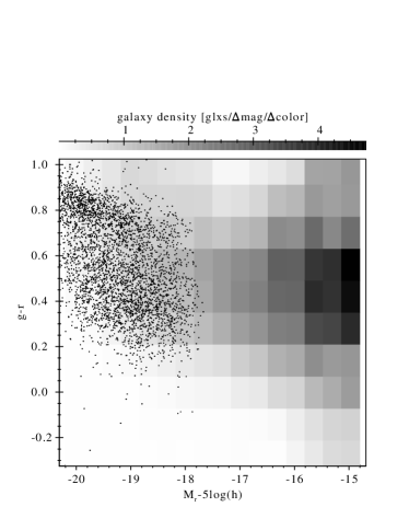
Figure 11.— Colour-magnitude distribution of excess counts of $-18<M_{r}<-15$ companions of bright primaries (sample S2-A) resulting from a background subtraction calculation.

The results shown in Table 2 show a better signal to noise ratio as more primaries comprise the subsamples. Bright primaries ($M_{r}<-21.5$) host on average 7 satellites while low luminosity primaries ($-21.5<M_{r}<-20.5$) host a mean of only 1 satellite galaxy per primary. In Fig. 8 we show the $r$–band luminosity distribution of satellites around bright primaries ($M_{r}<-21.5$) and primaries with intermediate luminosities ($-21.5<M_{r}<-20.5$, sample S1). We also show in this Figure Schechter function fits computed using the universal value of $M_{\star}$, whith a faint end slope parameter $\alpha=-1.3\pm 0.2$, obtained using a maximum likelihood method. These luminosity functions indicate a lack of a dominant population of faint satellites, which would be reflected in much larger negative values of the $\alpha$ parameter. These results contrast with those obtained for groups/clusters of galaxies (Popesso et al., 2005; González et al., 2006), where the faint component contribution $M_{r}>-18.$ to a double Schechter fitting gives slope values as steep as $\alpha\sim-2$.

We have also analyzed the dependence of the results on primary colour index. As mentioned in Section 2.1 we have used the threshold $g-r=0.8$ to divide the samples of primaries. Similarly, we find a larger population of satellites associated to red hosts, with a slightly stepper luminosity distribution at the faint end (Fig. 9). We have studied the radial density profiles of red and blue satellites around the different samples of primaries, finding that the system of blue satellites is in all cases, more extended than that of the red ones by approximately 30 per cent. Luminosity distributions of red and blue satellites are shown for the brightest hosts in Fig. 10.

We also computed a colour–magnitude diagram for the satellites obtained by means of applying the background subtraction method simultaneously to these two variables. The results are shown in Fig. 11 for sample S2-A-a, where it can be appreciated the smooth extension of the spectroscopic data onto fainter objects obtained by our statistical approach.

5. Testing the method with numerical simulations

The success of a background subtraction method relies on the signal-to-background strength from satellites around bright galaxies, providing the overdensity enhancement obtained in the stacking procedure. However, the superposition of large scale structures projected onto the sky could affect the uniformity of the background. In order to estimate the ability of the method to correctly reproduce the actual distributions of satellite galaxies in SDSS-DR7 data, we have tested it on a mock catalogue derived from a numerical simulation using similar conditions than that applied to the observations. We constructed the mock catalogue within a $\pi/2$ sterradians light-cone, based on a semianalytic model of galaxy formation (Croton et al., 2006) at redshift zero in the Millennium simulation (Springel et al., 2005), which is publicly available from the German Virtual Observatory . This solid angle corresponds to approximately half the area covered by the spectroscopic DR7 catalogue of galaxies and the $z=0$ snapshot was replicated 8 times along the axes to achieve a suitable depth.

Since the output of the semianalytic model includes magnitudes in the ugriz photometric system, the mock spectroscopic catalogue is obtained directly by selecting galaxies brighter than the limiting apparent magnitude of the Sloan spectroscopic galaxy catalogue, r=$17.77$. From the mock spectroscopic catalogue we extract a sample of mock primaries using similar criteria than in Section 2 which will be used as centers in the following analysis. For each galaxy, a redshift is assigned by placing a fiducial observer at one corner, and determining the comoving distance to the observer and the peculiar velocity of the galaxy. The evolution corrected $r$–band magnitude is:

$$M_{r}=-2.5\,\log(L)+E-5\,\log(h),$$

where $E$ is given by Blanton et al. (2003b).

For the adopted r–band limiting magnitude $21.5$ of the photometric sample, the maximum redshift of the mock should be $1.2$, corresponding approximately to the distance at which an intrinsically luminous galaxy is observable within the absolute magnitude range explored, $-18.5<M_{r}<-14.5$. Although the lack of evolution in both galaxies and structure is a drawback of the mock catalogue, it serves as a strong test of the method given that in this case there is a larger clustering amplitude of high redshift structures (i.e. more structures along the line of sight) compared to a mock catalogue with consistent evolution in clustering.

Since we have adopted a colour cut $g-r<1$ in SDSS data to reduce background noise, we have performed an appropriate noise reduction in the mock catalogue using a Monte Carlo procedure in order to reproduce the conditions of the observations. We have considered photometric redshifts obtained by O’Mill et al. (2010) (private communication) for the SDSS-DR7 galaxy sample to derive the fraction $P(z)$ of galaxies with observed colour index $g-r<1$ as a function of redshift. A suitable fit to this probability is given by $P(z)=1-2.381\,(z-0.08)$ which rejects about half the galaxies with $g-r>1$ at $z\sim 0.3$. We have adopted this statistical procedure instead of a direct filtering of galaxies by the observed colour in the photometric mock catalogue, given that this would be model dependent, also requiring reliable K correction for the semianalytic galaxies. We also checked that our results are not strongly dependent on the precise assumed $P(z)$, so that little modifications in the fit have minimum impact in the obtained radial and luminosity distributions.

We have firstly tested if the galaxy density profile around primaries derived by the background subtraction method is able to reproduce the actual projected 3D profile. For this aim we have computed the projected radial distribution of galaxies around centers reproducing sample S2-A-a in the mock catalogue using the real space positions in order to test the reproducibility of the results through the background subtraction method. We show the results obtained for this sample (S2-A-a) in the mock catalogue since it presents the stronger signal. The results described in this section, however, does not depend on the chosen subsample. The criteria to select satellites in the mock 3D catalogue, was chosen so that a galaxy from the semi–analytic output is considered a satellite if it is within $3R_{vir}$ of the host dark matter halo of the primary galaxy, in three–dimensional space. This is consistent with the criteria adopted in Section 4.2 for the selection of the region where the signal is studied in the observational samples. In Fig. 12 we show the good agreement of the projected 3D and background subtraction derived profiles, indicating that the method is effective in recovering the true projected profile of companion galaxies.

The luminosity distribution of satellite galaxies were computed using the halo membership and galaxy luminosities in the mock catalogue, and compared to the luminosity distribution of galaxies obtained with the background subtraction in the region $100<R_{p}/kpc<660$ corresponding to this sample. The cumulative luminosity distribution obtained through the background subtraction procedure reproduces the true underlying distribution remarkably well, as can be appreciated in Fig. 13. We also display in the inset of this Figure the differential distributions, which also present a general consistency. Although a small difference is present between the two samples, that does not affect the shape of the luminosity distribution and the determination of the Schechter parameter, since this is due to a small difference in the first magnitude bin. The method also succeeds in reproducing the discontinuity at $M_{r}\approx-17.6$, due to the absolute limiting magnitude in the parent semianalytic galaxy catalogue.

These tests discard the possibility that background structures affect the shape of the obtained luminosity distributions, so that the faint end slopes are computed on firm statistical basis. We stress the fact, however, that this procedure is reliable provided that adequate selection criteria have been imposed to the data. Since primary galaxies in our samples span a redshift range much smaller than most of galaxies contributing to background counts, the procedure used to compute radial and luminosity distributions performs in convenient conditions, as our tests in the mock catalogue have shown. This result is in conformity with previous tests of the method in less favorable conditions as in the determination of cluster luminosity functions (Valotto et al., 2001; Muñoz et al., 2009).

6. Discussion and conclusions

We have carried out different statistical analyses to infer properties of faint satellite galaxies in the projected distance range $100<r_{p}/\rm{kpc}<3<R_{vir}>$, associated to bright primaries taken from SDSS with redshift $z<0.1$ To this end, we have implemented a background subtraction method on faint galaxies with photometric information, that are close in projection to galaxies with measured redshifts. The innermost region of the satellite systems is not accessible using the proposed background subtraction method and data from the photometric galaxy catalogue. However, assuming a power law profile for satellites and considering objects outside 100 kpc radial distance from the host, we can study more than 80 per cent of satellites. We have used a mock galaxy catalogue based on a semianalytic model of galaxy formation from the Millennium simulation to test the method with similar conditions than in the observational data. According to the results of the tests performed, the method is able to provide a good estimation of the true distributions of luminosities and projected radial galaxy density as a function of the distances to the host (Fig. 12 and Fig. 13). In our mock catalogue we test how the projection of background structures affect our measurement in a worst case scenario. We conclude that these structures does not affect the shape of the luminosity distribution, provided that central galaxies are sufficiently bright ($M_{p}<-20.5$) and isolated, and a colour cut $g-r<1$ is imposed to satellites. We also find it important to define an adequate maximum radius, using theoretical insight and mock catalogues to calibrate the values of $R_{max}$ for each sample.

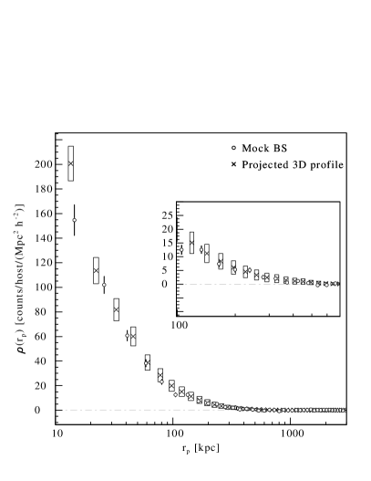
Figure 12.— Projected density profile of galaxies around primaries in the mock catalogue. Open circles correspond to results obtained by the background subtraction method, and filled circles correspond to the projection of the 3D density profile within the halos of each primary. We show in the inset figure, the region we actually use in this work. Since the mock catalogue is not affected by spurious photometric galaxy detections, we could also show the good agreement between both profiles at projected radius below $100$ kpc.

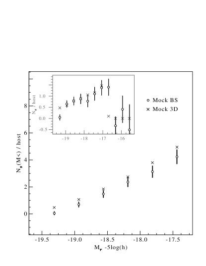
Figure 13.— Cumulative luminosity distribution of galaxies around primaries in the sample S2 of the mock catalogue. Open circles correspond to the results from the background subtraction method. Filled circles are the actual luminosity distribution of satellites within three times the virial radius of the primary galaxies. In the inset we show the differential luminosity distribution on a luminosity range beyond the completeness limit of the mock catalogue, where the background subtraction retrieve a distribution consistent with zero galaxies for $M_{r}>-17.$ in the Millennium semi–analytic catalogue.

In all samples of primaries (defined in Table 1) we detect an excess of faint galaxy counts and we can determine statistically the properties of companion objects associated to the central galaxy. We find that the radial density profiles of satellites are consistent with power laws of the form $\rho(r_{p})=Ar_{p}^{-\gamma}$, with $-2.4\lesssim\gamma\lesssim 1.1$ and that the maximum extent and amplitude of the overdensity depends on the primary luminosity and colour (see Fig. 6), as well as on galaxy luminosity (Fig. 5). The dependence of the number of satellites with $M_{r}<-14.5$ on host luminosity is strong: bright primaries with $M_{r}<-21.5$ host on average approximately 6 satellites, which is reduced to $\sim$1 satellite for S1 primaries (Table 2). Liu et al. (2010) investigate the probabilities of finding a Milky Way like galaxy to host satellites with luminosities similar to the Magellanic Clouds. The authors report that $8$ per cent of these galaxies have at least 2 satellites similar to the LMC and SMC. In order to compare with these results we computed the mean number of satellites in the magnitude range $-19.5<M_{r}<-14.5$ for Milky Way like primaries ($-21.4<M_{r}<-21.$), within $z=0.1$, using the previously described methodology. We find a $(3\pm 2)$ per cent probability to obtain systems similar to MW-LMC-SMC. This is consistent with the results presented in Liu et al. (2010), since we exclude in the analysis the central $100kpc$ region.

Recently, Wang et al. (2010) use a deep photometric sample around spectroscopically identified galaxies, and found that projected density profiles show a similar slope to the correlation function slope, independently of galaxy luminosity. Due to the different luminosity and redshift ranges considered between the work of Wang et al. (2010) and ours, a direct comparison is difficult to perform. While this paper was being reviewed, Guo et al. (2011) presented a complementary analysis of the luminosities of satellites of SDSS primary galaxies, finding a general agreement with our results.

The redshift range of the spectroscopic sample and the apparent magnitude limit of the photometric catalogue allows to obtain luminosity distributions in the range $-18.5<M_{r}<-14.5$. The derived luminosity distributions can be well described by Schechter function fits (Fig. 8). Our findings indicate that faint end slopes of the satellite luminosity functions are slightly rising ($\alpha=-1.3\pm 0.2$). This is in agreement with the luminosity distributions of galaxies in the local group, in the same magnitude range (Mateo, 1998). This result is valid for all samples and indicates that the population of satellites of bright isolated primaries are consistent with the nearly flat faint end slope of the global luminosity function as derived for the SDSS data (Blanton et al., 2003b; Baldry et al., 2005; Montero-Dorta & Prada, 2009). These findings contrast with the results obtained by similar methods in samples of clusters and groups where a significantly steep function is obtained ($\alpha\sim-2$ to $-1.5$, e.g. de Propris et al., 1995; Popesso et al., 2005; González et al., 2006). These results are expected, given the evidence from semianalytic models of galaxy formation that suggest that the total mass of a dark matter halo determines the normalization and shape of the luminosity function (Macciò et al., 2010).

References

- Abazajian et al. (2004) Abazajian, K., et al. 2004, AJ, 128, 502
- Abazajian et al. (2009) Abazajian, K. N., et al. 2009, ApJS, 182, 543
- Agustsson & Brainerd (2006) Agustsson, I., & Brainerd, T. G. 2006, ApJ, 644, L25
- Agustsson & Brainerd (2010) —. 2010, ApJ, 709, 1321
- Andreon et al. (2005) Andreon, S., Punzi, G., & Grado, A. 2005, MNRAS, 360, 727
- Ann et al. (2008) Ann, H. B., Park, C., & Choi, Y. 2008, MNRAS, 389, 86
- Baldry et al. (2005) Baldry, I. K., et al. 2005, MNRAS, 358, 441
- Barkhouse et al. (2007) Barkhouse, W. A., Yee, H. K. C., & López-Cruz, O. 2007, ApJ, 671, 1471
- Baugh (2006) Baugh, C. M. 2006, Reports of Progress in Physics, 69, 3101
- Benson (2010) Benson, A. J. 2010, Phys. Rep., 495, 33
- Benson et al. (2003) Benson, A. J., Bower, R. G., Frenk, C. S., Lacey, C. G., Baugh, C. M., & Cole, S. 2003, ApJ, 599, 38
- Bergvall et al. (2010) Bergvall, N., Zackrisson, E., & Caldwell, B. 2010, MNRAS, 405, 2697
- Bertschinger (1985) Bertschinger, E. 1985, ApJS, 58, 39
- Bertschinger (1994) Bertschinger, E. 1994, Physica D Nonlinear Phenomena, 77, 354
- Blanton et al. (2003a) Blanton, M. R., Lin, H., Lupton, R. H., Maley, F. M., Young, N., Zehavi, I., & Loveday, J. 2003a, AJ, 125, 2276
- Blanton et al. (2003b) Blanton, M. R., et al. 2003b, ApJ, 592, 819
- Blanton et al. (2005) —. 2005, AJ, 129, 2562
- Brainerd (2005) Brainerd, T. G. 2005, ApJ, 628, L101
- Chen (2008) Chen, J. 2008, A&A, 484, 347
- Chen et al. (2006) Chen, J., Kravtsov, A. V., Prada, F., Sheldon, E. S., Klypin, A. A., Blanton, M. R., Brinkmann, J., & Thakar, A. R. 2006, ApJ, 647, 86
- Christlein (2000) Christlein, D. 2000, ApJ, 545, 145
- Coil et al. (2006) Coil, A. L., et al. 2006, ApJ, 638, 668
- Cole et al. (1994) Cole, S., Aragon-Salamanca, A., Frenk, C. S., Navarro, J. F., & Zepf, S. E. 1994, MNRAS, 271, 781
- Collister & Lahav (2005) Collister, A. A., & Lahav, O. 2005, MNRAS, 361, 415
- Cooray & Milosavljevic (2005) Cooray, A., & Milosavljevic, M. 2005, ApJ, 627, L85
- Cooray & Sheth (2002) Cooray, A., & Sheth, R. 2002, Physics Reports, 372, 1
- Croton et al. (2006) Croton, D. J., et al. 2006, MNRAS, 365, 11
- de Propris et al. (1995) de Propris, R., Pritchet, C. J., Harris, W. E., & McClure, R. D. 1995, ApJ, 450, 534
- Font et al. (2008) Font, A. S., et al. 2008, MNRAS, 389, 1619
- Fukugita et al. (1996) Fukugita, M., Ichikawa, T., Gunn, J. E., Doi, M., Shimasaku, K., & Schneider, D. P. 1996, AJ, 111, 1748
- González et al. (2006) González, R. E., Lares, M., Lambas, D. G., & Valotto, C. 2006, A&A, 445, 51
- Górski et al. (2005) Górski, K. M., Hivon, E., Banday, A. J., Wandelt, B. D., Hansen, F. K., Reinecke, M., & Bartelmann, M. 2005, ApJ, 622, 759
- Gunn et al. (2006) Gunn, J. E., Siegmund, W. A., Mannery, E. J., Owen, R. E., Hull, C. L., Leger, R. F., & Carey, L. N. 2006, AJ, 131, 2332
- Guo et al. (2011) Guo, Q., Cole, S., Eke, V., & Frenk, C. 2011, ArXiv e-prints
- Hamilton & Tegmark (2004) Hamilton, A. J. S., & Tegmark, M. 2004, MNRAS, 349, 115
- Hansen et al. (2005) Hansen, S. M., McKay, T. A., Wechsler, R. H., Annis, J., Sheldon, E. S., & Kimball, A. 2005, ApJ, 633, 122
- Jones & Forman (1984) Jones, C., & Forman, W. 1984, ApJ, 276, 38
- Kang et al. (2006) Kang, X., Jing, Y. P., & Silk, J. 2006, ApJ, 648, 820
- Khochfar & Silk (2009) Khochfar, S., & Silk, J. 2009, MNRAS, 397, 506
- Klypin et al. (1999) Klypin, A., Kravtsov, A. V., Valenzuela, O., & Prada, F. 1999, ApJ, 522, 82
- Koposov et al. (2008) Koposov, S., et al. 2008, ApJ, 686, 279
- Kravtsov et al. (2004) Kravtsov, A. V., Gnedin, O. Y., & Klypin, A. A. 2004, ApJ, 609, 482
- Lares (2009) Lares, M. 2009, PhD thesis, FaMAF, UNC
- Li et al. (2007) Li, C., Jing, Y. P., Kauffmann, G., Börner, G., Kang, X., & Wang, L. 2007, MNRAS, 376, 984
- Lin et al. (2004) Lin, Y., Mohr, J. J., & Stanford, S. A. 2004, ApJ, 610, 745
- Lin et al. (2004) Lin, Y., Mohr, J. J., & Stanford, S. A. 2004, ApJ, 610, 745
- Liu et al. (2009) Liu, F. S., Mao, S., Deng, Z. G., Xia, X. Y., & Wen, Z. L. 2009, MNRAS, 396, 2003
- Liu et al. (2010) Liu, L., Gerke, B. F., Wechsler, R. H., Behroozi, P. S., & Busha, M. T. 2010, ArXiv e-prints
- Lupton et al. (2001) Lupton, R., Gunn, J. E., Ivezić, Z., Knapp, G. R., & Kent, S. 2001, in Astronomical Society of the Pacific Conference Series, Vol. 238, Astronomical Data Analysis Software and Systems X, ed. F. R. Harnden Jr., F. A. Primini, & H. E. Payne, 269–+
- Macciò et al. (2010) Macciò, A. V., Kang, X., Fontanot, F., Somerville, R. S., Koposov, S., & Monaco, P. 2010, MNRAS, 402, 1995
- Mateo (1998) Mateo, M. L. 1998, ARA&A, 36, 435
- Montero-Dorta & Prada (2009) Montero-Dorta, A. D., & Prada, F. 2009, MNRAS, 399, 1106
- Moore et al. (1999) Moore, B., Ghigna, S., Governato, F., Lake, G., Quinn, T., Stadel, J., & Tozzi, P. 1999, ApJ, 524, L19
- Muñoz et al. (2009) Muñoz, R. P., Padilla, N. D., & Barrientos, L. F. 2009, MNRAS, 392, 655
- Nichol et al. (2003) Nichol, R. C., Miller, C. J., & Goto, T. 2003, apss, 285, 157
- Nierenberg et al. (2011) Nierenberg, A. M., Auger, M. W., Treu, T., Marshall, P. J., & Fassnacht, C. D. 2011, ApJ, 731, 44
- Oemler (1974) Oemler, A. 1974, ApJ, 194, 1
- Okamoto et al. (2010) Okamoto, T., Frenk, C. S., Jenkins, A., & Theuns, T. 2010, MNRAS, 406, 208
- O’Mill et al. (2010) O’Mill, A., Duplancic, F., Lambas, D. G., & Sodré, L. 2010, MNRAS, submitted to, 00
- Ostriker & Tremaine (1975) Ostriker, J. P., & Tremaine, S. D. 1975, ApJ, 202, L113
- Pimbblet (2008) Pimbblet, K. A. 2008, Are dumbbell brightest cluster members signposts to galaxy cluster activity?, http://adsabs.harvard.edu/abs/2008arXiv0808.2093P
- Popesso et al. (2005) Popesso, P., Böhringer, H., & Voges, W. 2005, in Multiwavelength Mapping of Galaxy Formation and Evolution, ed. A. Renzini & R. Bender, 444–+
- Sales & Lambas (2005) Sales, L., & Lambas, D. G. 2005, MNRAS, 356, 1045
- Schechter (1976) Schechter, P. 1976, ApJ, 203, 297
- Simon & Geha (2007) Simon, J. D., & Geha, M. 2007, ApJ, 670, 313
- Skibba et al. (2010) Skibba, R. A., van den Bosch, F. C., Yang, X., More, S., Mo, H., & Fontanot, F. 2010, MNRAS, 1465
- Smith et al. (2005) Smith, G. P., Kneib, J., Smail, I., Mazzotta, P., Ebeling, H., & Czoske, O. 2005, MNRAS, 359, 417
- Smith et al. (2002) Smith, J. A., et al. 2002, AJ, 123, 2121
- Springel et al. (2005) Springel, V., et al. 2005, Nature, 435, 629
- Stoughton et al. (2002) Stoughton, C., Lupton, R. H., Bernardi, M., Blanton, M. R., Burles, S., Castander, F. J., Connolly, A. J., & Eisenstein, D. J. 2002, AJ, 123, 485
- Strauss et al. (2002) Strauss, M. A., Weinberg, D. H., Lupton, R. H., Narayanan, V. K., Annis, J., Bernardi, M., Blanton, M., & Burles, S. 2002, AJ, 124, 1810
- Strigari et al. (2007) Strigari, L. E., Bullock, J. S., Kaplinghat, M., Diemand, J., Kuhlen, M., & Madau, P. 2007, ApJ, 669, 676
- Swanson et al. (2008) Swanson, M. E. C., Tegmark, M., Hamilton, A. J. S., & Hill, J. C. 2008, MNRAS, 387, 1391
- Tal & van Dokkum (2011) Tal, T., & van Dokkum, P. 2011, 1102.4330
- Tollerud et al. (2011) Tollerud, E. J., Boylan-Kolchin, M., Barton, E. J., Bullock, J. S., & Trinh, C. Q. 2011, ArXiv e-prints
- Tollerud et al. (2008) Tollerud, E. J., Bullock, J. S., Strigari, L. E., & Willman, B. 2008, ApJ, 688, 277
- Trentham & Tully (2002) Trentham, N., & Tully, R. B. 2002, MNRAS, 335, 712
- Trentham & Tully (2009) —. 2009, MNRAS, 398, 722
- Tully & Trentham (2008) Tully, R. B., & Trentham, N. 2008, AJ, 135, 1488
- Vale & Ostriker (2006) Vale, A., & Ostriker, J. P. 2006, MNRAS, 371, 1173
- Valotto et al. (2001) Valotto, C. A., Moore, B., & Lambas, D. G. 2001, ApJ, 546, 157
- Viola et al. (2008) Viola, M., Monaco, P., Borgani, S., Murante, G., & Tornatore, L. 2008, MNRAS, 383, 777
- Wang et al. (2010) Wang, W., Jing, Y. P., Li, C., Okumura, T., & Han, J. 2010, ArXiv e-prints
- Weinmann et al. (2006) Weinmann, S. M., van den Bosch, F. C., Yang, X., & Mo, H. J. 2006, MNRAS, 366, 2
- White (1976) White, S. D. M. 1976, MNRAS, 174, 19
- White & Frenk (1991) White, S. D. M., & Frenk, C. S. 1991, ApJ, 379, 52
- Willman et al. (2002) Willman, B., Dalcanton, J., Ivezic, Z., Jackson, T., Lupton, R., Brinkmann, J., Hennessy, G., & Hindsley, R. 2002, ApJ, 123, 848
- Yang et al. (2005) Yang, X., Mo, H. J., van den Bosch, F. C., Weinmann, S. M., Li, C., & Jing, Y. P. 2005, MNRAS, 362, 711
- Zibetti et al. (2004) Zibetti, S., White, S. D. M., & Brinkmann, J. 2004, MNRAS, 347, 556, Mon.Not.Roy.Astron.Soc.347:556-568,2004