Numerical Tests of the Improved Fermilab Action

Abstract:

Recently, the Fermilab heavy-quark action was extended to include dimension-six and -seven operators in order to reduce the discretization errors. In this talk, we present results of the first numerical simulations with this action (the OK action), where we study the masses of the quarkonium and heavy-light systems. We calculate combinations of masses designed to test improvement and compare results obtained with the OK action to their counterparts obtained with the clover action. Our preliminary results show a clear improvement.

1 Introduction

Simulating heavy quarks in lattice QCD is a challenging problem, because the quark mass $m_{Q}$ and the accessible ultraviolet cutoff $a^{-1}$ are comparable. Special care is needed to handle discretization errors [1]. In order to make accurate and reliable calculations of many Standard Model parameters involving heavy quarks, one needs not only computer power but also methodological improvements of the quark actions used. One line of attack is the Fermilab method [2], which starts with the clover action [3] for Wilson fermions [4]. In the original work, interactions through dimension five were considered. More recently, we extended the Fermilab method to an action (the OK action) with dimension-six and -seven interactions [5, 6].

Using power counting as a guide, Ref. [5] estimated that the OK action should reduce discretization effects for heavy quarks to $\sim 1\%$ on, say, the MILC asqtad ensembles [7]. In this paper, we present the first numerical results obtained with the OK action, to test whether the theoretical improvement is realized in practice. We compute combinations of rest masses and kinetic masses designed to test the improvement, without the need to tune the input parameters.

In Sec. 2, we briefly discuss and present the OK action. Section 3 contains the details of the simulations and our preliminary results for an inconsistency $I$ [8], and for the hyperfine splittings between rest and kinetic masses for the heavy-heavy and heavy-light systems. We discuss our results and future plans in section 4.

2 OK Action and Tadpole Improvement

In this section, we briefly describe the OK action, including the tadpole improvement [9] used in the simulation. In general, the Fermilab formalism calls for separate couplings for spatial and temporal interactions. Fermilab actions have a smooth transition to the $m_{0}a\to 0$ and $m_{0}a\to\infty$ limits, but the short-distance coefficients depend on $m_{0}a$, $\zeta$ and the spatial Wilson parameter $r_{s}$ in a non-trivial way [2]. This action reduces the discretization errors to $\mathrm{O}(a^{2}\Lambda^{2}b(m_{Q}a))$, where $b$ is a function that is bounded for all $m_{Q}a$. The OK action includes higher dimensional operators to further reduce the lattice spacing errors.

Reference [5] starts by considering all the operators of dimension six and seven with two effective field theories in mind: heavy-quark effective theory (HQET) and the nonrelativistic QCD (NRQCD), appropriate to heavy-light and heavy-heavy systems, respectively. The interactions are classified in powers of $\lambda$ (HQET, $\lambda\sim\Lambda/m_{Q}$, $\Lambda a$) or $v$ (NRQCD, relative internal velocity). Once all the independent operators are identified, the redundant ones are eliminated by means of field transformations, and the remaining couplings $c_{i}$ are determined via tree-level matching. Together with the one-loop matching of the dimension five chromomagnetic interaction, this action is expected to bring the discretization errors below the one-percent level [5].

For coding, and especially for tadpole improvement of the couplings, it is convenient to write the OK action in the hopping-parameter form:

$$S = \sum_{x}\bar{\psi}_{x}\psi_{x}-\kappa_{t}\sum_{x}\bar{\psi}_{x}(1-\gamma_{4})T_{4}\psi_{x}-\kappa_{t}\sum_{x}\bar{\psi}_{x}(1+\gamma_{4})T_{-4}\psi_{x}$$

$$- \kappa_{t}\sum_{x,i}\bar{\psi}_{x}[(r_{s}\zeta+8c_{4})-\gamma_{i}(\zeta-2c_{1}-12c_{2})]T_{i}\psi_{x}$$

$$- \kappa_{t}\sum_{x,i}\bar{\psi}_{x}[(r_{s}\zeta+8c_{4})+\gamma_{i}(\zeta-2c_{1}-12c_{2})]T_{-i}\psi_{x}$$

$$+ \kappa_{t}\sum_{x}\bar{\psi}_{x}[2c_{4}+\gamma_{i}(c_{1}+2c_{2})]T_{i}^{2}\psi_{x}-\kappa_{t}(c_{B}\zeta+16c_{5})\sum_{x}\bar{\psi}_{x}i\bm{\Sigma}\cdot\bm{B}_{\rm lat}\psi_{x}$$

$$+ \kappa_{t}\sum_{x}\bar{\psi}_{x}[2c_{4}-\gamma_{i}(c_{1}+2c_{2})]T_{-i}^{2}\psi_{x}-\kappa_{t}c_{E}\zeta\sum_{x}\bar{\psi}_{x}i\bm{\alpha}\cdot\bm{E}_{\rm lat}\psi_{x}$$

$$+ \kappa_{t}c_{2}\sum_{x,i\neq j}\bar{\psi}_{x}\gamma_{i}\{T_{i}\!-\!T_{-i},T_{j}\!-\!T_{-j}\}\psi_{x}+2\kappa_{t}c_{5}\sum_{x}\bar{\psi}_{x}\sum_{i}\sum_{i\neq j}\{i\Sigma_{i}B_{i\rm{lat}},(T_{j}\!+\!T_{-j})\}\psi_{x}$$

$$+ 2\kappa_{t}c_{3}\sum_{x}\bar{\psi}_{x}\{\bm{\gamma}\cdot\bm{D}_{\rm lat},i\bm{\Sigma}\cdot\bm{B}_{\rm lat}\}\psi_{x}+2\kappa_{t}c_{EE}\sum_{x}\bar{\psi}_{x}\{\gamma_{4}D_{4\rm{lat}},\bm{\alpha}\cdot\bm{E}_{\rm lat}\}\psi_{x}$$

where $T_{\pm\mu}\psi(x)=U_{\pm\mu}(x)\psi(x\pm a\hat{\mu})$ with $U_{-\mu}(x)=U^{\dagger}_{\mu}(x-a\hat{\mu})$ and

$$m_{0}a=\frac{1}{2\kappa_{t}}-(1+3r_{s}\zeta+18c_{4}).$$ (1)

For further details and the matching conditions for the couplings $c_{i}$, we refer the reader to Ref. [5].

Given the large one-loop corrections that can arise in lattice perturbation theory [9], before using the OK action in a numerical simulation we apply tadpole improvement to the matched couplings. To carry out the tadpole improvement, it is convenient to write $T_{\pm\mu}=u_{0}[T_{\pm\mu}/u_{0}]=u_{0}\tilde{T}_{\pm\mu}$ where $u_{0}$ factors are absorbed into the couplings $\tilde{c}_{i}$. In this way, one finds the relations between bare and tadpole improved coefficients

$$\tilde{\kappa}_{t} = u_{0}\kappa_{t},$$ (2)

$$\tilde{r}_{s}\tilde{\zeta}+8\tilde{c}_{4} = r_{s}\zeta+8c_{4}$$ (3)

$$\tilde{\zeta}-2\tilde{c}_{1}-12\tilde{c}_{2} = \zeta-2c_{1}-12c_{2}$$ (4)

$$\tilde{c}_{4} = u_{0}c_{4},$$ (5)

$$\tilde{c}_{1}+2\tilde{c}_{2} = u_{0}(c_{1}+2c_{2})$$ (6)

$$\tilde{c}_{2} = u_{0}c_{2},$$ (7)

$$\tilde{c}_{B}\tilde{\zeta}+16\tilde{c}_{5} = u_{0}^{3}(c_{B}\zeta+16c_{5})$$ (8)

$$\tilde{c}_{E} = u_{0}^{3}c_{E},$$ (9)

$$\tilde{c}_{3} = u_{0}^{4}c_{3},$$ (10)

$$\tilde{c}_{EE} = u_{0}^{4}c_{EE},$$ (11)

where the last two follow because every term in the anticommutators has five links, while one power of $u_{0}$ is absorbed, as usual, into $\tilde{\kappa}_{t}$. The matching conditions of Ref. [5] are then used, substituting

$$\tilde{m}_{0}a=\frac{1}{2\tilde{\kappa}_{t}}-(1+3\tilde{r}_{s}\tilde{\zeta}+18\tilde{c}_{4})$$ (12)

for $m_{0}a$. Another condition for $\tilde{c}_{5}$ is needed, but it is not simple to express. In the expansion of $B_{i{\rm lat}}$ in terms of $T$s, one finds that $\bar{\psi}_{x}\{i\Sigma_{i}B_{i{\rm lat}},(T_{j}+T_{-j})\}\psi_{x}$, $j\neq i$, has terms with both 3 and 5 links. The 3-link terms arise from $T_{\pm\mu}T_{\mp\mu}=1$. In the $c_{3}$ and $c_{EE}$ interactions, each 3-link term appears twice, but with opposite sign, while here they have the same sign. Coding this operator with the correct $u_{0}$ factors is currently underway with USQCD software [10].

3 Simulations and Tests

We performed simulations on a “medium coarse” ($a\approx 0.15$ fm) $16^{3}\times 48$ lattice with 2+1 flavors of sea quarks, $(am_{l},am_{s})=(0.029,0.0484)$. From Ref. [11], we had data available with the clover action, and here we used the OK action with similar statistics, 500 configurations with 4 time sources per configuration. For the results presented here, we tadpole-improved the $\bar{\psi}_{x}\{i\Sigma_{i}B_{i{\rm lat}},(T_{j}+T_{-j})\}\psi_{x}$, $j\neq i$, interaction with $\tilde{c}_{5}=u_{0}^{4}c_{5}$, pending completion of the code with proper tadpole improvement. We also choose $\tilde{r_{s}}=\tilde{\zeta}=\tilde{c}_{B}=1$. This choice fixes the value of $\tilde{c}_{4}$ and $\tilde{c}_{5}$ while the rest of the coefficients also depend on the choice of $\tilde{\kappa}_{t}$.

Since the action is designed to improve $O(p^{4})$ terms, we need to find observables to test these improvements. One such quantity is a combination of masses introduced in Ref. [8] and later discussed in Ref. [12]. Writing the rest and kinetic meson masses $M_{1\bar{Q}q}$ and $M_{2\bar{Qq}}$ as

$$M_{1\bar{Q}q} = m_{1\bar{Q}}+m_{1q}+B_{1\bar{Q}q},$$ (13)

$$M_{2\bar{Q}q} = m_{2\bar{Q}}+m_{2q}+B_{2\bar{Q}q},$$ (14)

where the $m$s are quark masses and the $B$s are binding energies, Ref. [8] introduced the “inconsistency combination”

$$I:=\frac{2\delta M_{\bar{Q}q}-(\delta M_{\bar{Q}Q}+\delta M_{\bar{q}q})}{2M_{2\bar{Q}q}}=\frac{2\delta B_{\bar{Q}q}-(\delta B_{\bar{Q}Q}+\delta B_{\bar{q}q})}{2M_{2\bar{Q}q}}$$ (15)

where $\delta M=M_{2}-M_{1}$, $\delta B=B_{2}-B_{1}$. The rightmost expression follows from the definitions.

The binding energies $B_{2}$ stem from the $p^{4}$ terms in the action [12]. By design, the the OK action improves these terms, compared with the clover action. Ideally, $\delta B$s and, hence, $I$ should vanish, and we expect $I$ to be smaller with an improved action. In order to compare the OK action with the clover action, we compute the rest and kinetic masses of heavy-light and heavy-heavy systems at four different hopping-parameter values, $\tilde{\kappa}_{t}=0.042,0.040,0.038,0.036$. Table 1 lists the obtained pseudoscalar kinetic masses, to show the range of physical mass covered here.

Table 1: Approximate values of the kinetic masses for the heavy-light and heavy-heavy systems obtained with the OK action. Thus, 0.042 is in the charm region and 0.036 is not yet in the bottom region.

$\tilde{\kappa}_{t}$	$M_{2}^{\mathrm{PS}}$ (Heavy-Light) [MeV]	$M_{2}^{\mathrm{PS}}$ (Heavy-Heavy) [MeV]
0.036	4418	7332
0.038	3500	5778
0.040	2680	4227
0.042	1876	2736

Figure 1 shows our results for the inconsistency $I$, together with results from an earlier study with the clover action [11].

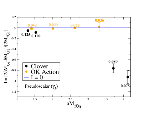
Figure 1: Comparison of the inconsistency $I$ between the OK action and the clover action. For the clover action $\kappa=0.122$ and $\kappa=0.076$ correspond to tuned $\eta_{c}$ and $\eta_{b}$ masses.

For simplicity, and without serious loss in the strength of the test, we omit the light-light mass difference $\delta M_{\bar{q}q}$. As one can see, the clover action suffers from serious deviations from $I\neq 0$, especially for hopping parameters in the $b$-quark region. On the other hand, the OK action’s inconsistency is statistically consistent with $I=0$ up to the largest masses considered.

Another way to see the effects of improvement is to look at the hyperfine splittings. Let us define

$$\Delta_{1} = M_{1}^{\mathrm{V}}-M_{1}^{\mathrm{PS}},$$ (16)

$$\Delta_{2} = M_{2}^{\mathrm{V}}-M_{2}^{\mathrm{PS}},$$ (17)

where V and PS denote vector and pseudoscalar mesons. The rest-mass splitting $\Delta_{1}$ is accurate at the tree level, thanks to the clover term, but the kinetic-mass splitting $\Delta_{2}$ has contributions from higher-dimension corrections such as $\{\bm{\gamma}\cdot\bm{D},i\bm{\Sigma}\cdot\bm{B}\}$, which are improved (unimproved) with the OK (clover) action.

In Fig. 2 we plot $a\Delta_{2}$ vs. $a\Delta_{1}$ for quarkonium at the same values of $\tilde{\kappa}_{t}$ as above.

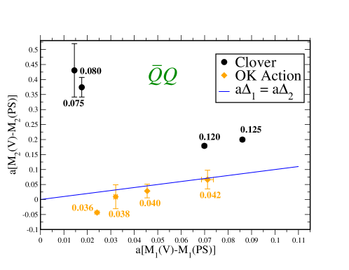
Figure 2: Kinetic-mass hyperfine splitting vs. rest-mass hyperfine splitting for the heavy-heavy system.

Ideally, the data would land on the line $a\Delta_{2}=a\Delta_{1}$. We see that the OK data fare much better than the clover data. In Fig. 3 we plot $a\Delta_{2}$ vs. $a\Delta_{1}$ for a heavy-light meson.

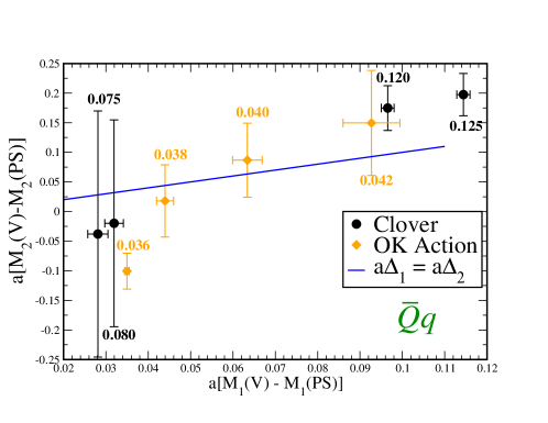
Figure 3: Kinetic-mass hyperfine splitting vs. rest-mass hyperfine splitting for the heavy-light system.

In this case, the clover action fares well to begin with, and our statistical errors are not small enough to test whether the OK action is an improvement.

4 Outlook

Our preliminary analysis of the OK action is encouraging. It shows clear improvements in the inconsistency $I$ and the kinetic-mass hyperfine splittings in the heavy-heavy system. For the hyperfine splitting in the heavy-light system, the improvement is not yet clear, because the clover action already works well, so a decisive test requires higher statistics. The code for the OK inverter is still under development. The next step is to finish coding of the $c_{5}$ term with the correct $u_{0}$ factors, to be followed by a thorough optimization. Thereafter, we plan on using the OK action for charm and bottom physics.

Computations for this work were carried out in part on facilities of the USQCD Collaboration, which are funded by the Office of Science of the United States Department of Energy. This work was supported in part by the U.S. Department of Energy under Grants No. DE-FC02-06ER41446 (C.D., M.B.O), by the National Science Foundation under Grants No. PHY-0555243, No. PHY-0757333, No. PHY-0703296 (C.D., M.B.O), and by Universities Research Association, Inc. (M.B.O.). Fermilab is operated by Fermi Research Alliance, LLC, under Contract No. DE-AC02-07CH11359 with the U.S. Department of Energy.

References

- [1] A. S. Kronfeld, Nucl. Phys. Proc. Suppl. 129 (2004) 46 [arXiv:hep-lat/0310063].
- [2] A. X. El-Khadra, A. S. Kronfeld, and P. B. Mackenzie, Phys. Rev. D 55, 3933 (1997) [arXiv:hep-lat/9604004].
- [3] B. Sheikholeslami and R. Wohlert, Nucl. Phys. B 259, 572 (1985).
- [4] K. G. Wilson, in New Phenomena in Subnuclear Physics, edited by A. Zichichi (Plenum, New York, 1977).
- [5] M. B. Oktay and A. S. Kronfeld, Phys. Rev. D 78, 014504 (2008) [arXiv:0803.0523 [hep-lat]].
- [6] A. S. Kronfeld and M. B. Oktay, PoS LAT2006, 159 (2006) [arXiv:hep-lat/0610069]; M. B. Oktay et al., Nucl. Phys. B Proc. Suppl. 119, 464 (2003) [arXiv:hep-lat/0209150]; 129, 349 (2004) [arXiv:hep-lat/0310016].
- [7] A. Bazavov et al., Rev. Mod. Phys. 82 (2010) 1349 [arXiv:0903.3598 [hep-lat]].
- [8] S. Collins, R. G. Edwards, U. M. Heller and J. H. Sloan, Nucl. Phys. Proc. Suppl. 47, 455 (1996) [arXiv:hep-lat/9512026].
- [9] G. P. Lepage and P. B. Mackenzie, Phys. Rev. D 48 (1993) 2250 [arXiv:hep-lat/9209022].
- [10] http://www.usqcd.org/.
- [11] T. Burch et al. [Fermilab Lattice and MILC Collaborations], Phys. Rev. D 81, 034508 (2010) [arXiv:0912.2701 [hep-lat]].
- [12] A. S. Kronfeld, Nucl. Phys. Proc. Suppl. 53, 401 (1997) [arXiv:hep-lat/9608139].