Geometric Algorithms for Identifying and Reconstructing Galaxy Systems

1 Introduction

The recognition of patterns and structures in a given point distribution is common challenging task in science and engineering. In astronomy, in particular, the night-sky itself offers a natural set of points suitable for topological analysis. Ancient astronomers grouped bright stars into simple patterns (constellations) whose form and configuration could be easily identified. For a long time, this simple eyeball classification has provided us with useful signposts for tracking the flow of the seasons or for orienting sea travellers.

Modern astronomers detect and catalogue the structures traced by galaxies on the grand scale of the universe, as well. This activity has actually become a discipline on itself called cosmography. However, since the human eye and human mind respond in a biased way to contrast and continuity, cosmography is not based on visual impressions, as in the old days, but on a quantitative statistical description of patterns. What has remained unchanged across time is the importance of this activity. For example, by measuring in an objective and reproducible way the large-scale spatial arrangement of galaxies we can have access to fundamental information about the universe’s mass content and distribution. Additionally, an unbiased reconstruction of the galaxy distribution provides us with a quantitative characterization of the environment in which galaxies live, i.e. groups, cluster, super-clusters, filaments and walls.

Groups and clusters of galaxies, in particular, provide ideal laboratories for studying many aspects of the physics of galaxies within a well-defined, controlled, environment. Therefore, the finer their identification and reconstruction, the finer the scientific issues one can resolve. For example, one can evaluate the effects of the environment on the evolution of galaxies and assess which physical mechanisms (for example ram pressure stripping of gas, galaxy-galaxy merging, etc.) are (or not) crucial in determining the present day aspect of galaxies. Answering these key topics will provide us with insights concerning the nature of galaxy evolution itself and will clarify whether galaxy properties were established early on when galaxies first assembled (the so-called “nature” hypothesis), or whether they are the present day cumulative end product of multiple environmental processes operating over the entire history of the universe (the “nurture” scenario).

The specific theme of this review is to describe various algorithms developed by cosmologists for identifying and reconstructing groups and clusters of galaxies out of the general galaxy distribution. To this aim, I will follow the progression of clusters detection techniques through time, from the very first visual-like algorithms to the most performant geometrical methods available today. This will allow readers to understand the development of the field as well as the various issues and pitfalls we are confronted with. In particular, I will emphasize some recently developed, optimal detection techniques which are based on the Voronoi and Delaunay geometric models. I will overview their relative strengths and limitations and compare their performances with the more standard cluster-finding tools.

This paper is structured as follows: in §2 I will introduce the notion of galaxy groups and clusters, briefly presenting their main astrophysical properties. In §3 I will survey some general group/cluster identification tools traditionally used by astronomers for detection in both 2 and 3 dimensional space. Voronoi-Delaunay based cluster-finding algorithms are presented in §4. Conclusions are drawn in §5.

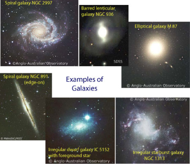
Figure 1: Galaxies have a variety of morphologies, stellar content and kinematics. Elliptical galaxies are pressure-supported systems which contain an old population of stars having red colors (cold surface temperatures). The fundamental building blocks of centrifugally supported spirals and dynamically irregular galaxies are younger and hotter (bluer) stars. (Credit: Anglo-Australian Observatory, D. Malin, IAC, RGO and SDSS)

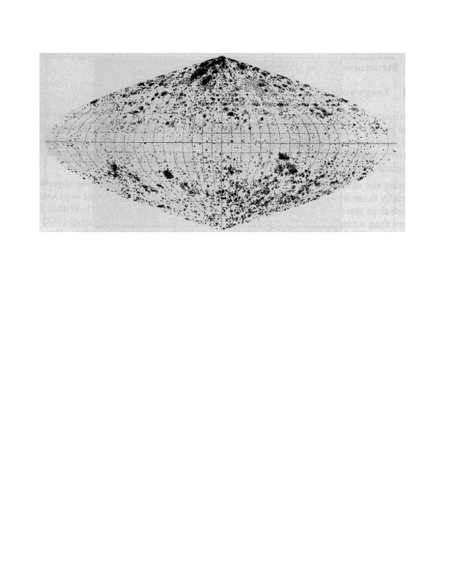
Figure 2: Charlier’s map of 11,475 nebulae charly , based on the New General Catalogue and the two Index Catalogues (D1 ,D2 ,D3 )

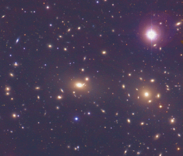
Figure 3: The Coma cluster - Abell 1656 - is an example of a rich regular cluster. Here the center of the cluster is shared between the two bright elliptical galaxies (the two bright objects at the center of the image). This cluster is 7Mpc in diameter and is thought to contain almost 2000 galaxies. The bright object in the upper right is a star from our own galaxy. Despite its regularity Coma is actually a merger of at least three smaller groups (e.g. ada ). Irregular clusters can also have a prominent bright central galaxy (and can sometimes be a giant elliptical galaxy) but are more disorganized in appearance. There is also no centralized concentration of galaxies near the center of the cluster.

2 What is a cluster?

According to the relativistic theory of gravity, matter is smoothly distributed, anchored to space and expanding with the metric of the universe. In particular, on small cosmological scales, theory predicts desitter and observations confirms hubble that the redshift $z$ between any two given matter particles is proportional to their separation $r$ via the relation

$$cz=Hr$$ (1)

where c is the speed of light and $H$ the Hubble constant. The Doppler formula ($V=cz$) allows us to re-interpret the redshift as a measure of the recession velocity of galaxies in the local universe. As a result, the Hubble relation of eq. (1) which characterizes the local expansion properties of the universe, also describes the apparent outward radial flow of galaxies as measured by a terrestrial observer.

Galaxies, however, the basic building blocks of the universe (see Fig. 1), are not evenly distributed throughout the space. The variance of the counts in arbitrary cells randomly thrown in the universe is larger than what we would expect from a purely Poissonian process. This is graphically seen in figure 2 which shows a map of galaxies derived by Charlier (1922) charly . Historically, this map represented one of the first ever pictures of an all-sky distribution of galaxies (or nebulae as they where called at that time). Commenting this plot, Charlier wrote: a glance at this plate suffices for stating how the Milky Way, which is designed by the great axis of the chart is systematically avoided by the nebulae. A remarkable property of the image is that the nebulae seem to be piled up in clouds (as also the stars in the Milky Way). Such a clouding of the nebulae may be a real phenomenon, but it may also be an accidental effect….

We now know that such a “clouding of nebulae” is not a spurious projection effect. Local gravitational perturbations tend to make receding galaxies slow down and clump together in small groups and sometimes in enormous complexes. Major collections (up to several thousands) of galaxies are called galaxy clusters. Actually, the universe is not composed of two distinct classes of objects: single galaxies and galaxies in groups. The long range action of the gravitational field introduces a strong correlation in the matter density field on scales less than $5$ Mpc. As a result, and as far as the local universe is concerned, galaxies are preferentially found in structures ranging from pairs (or binary systems) and triplets, through small groups, up to rich (and rare) clusters. Moreover, clusters themselves are often associated within larger gravitational structures called super-clusters. In this picture virtually no galaxies in the universe can be considered to be truly isolated.

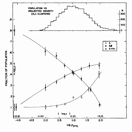
Figure 4: The morphology-density relation The fraction of ellipticals (old star galaxies), lenticulars and spirals (young star galaxies) as a function of the projected density. The upper histogram shows the number distribution of the galaxies over the bins of projected density. (Taken from dressler .)

In models for the gravitational formation of structure, the smallest density perturbations in an otherwise smooth universe collapse first and eventually build the largest structures, rich groups and clusters of galaxies. The most massive conglomerations of galaxies are therefore not only the largest gravitationally bound systems we know, but also the most recent objects to have arisen in the hierarchical structure formation of the universe.

A regular cluster can be described, at first order, as a spherically symmetric object in hydrostatic equilibrium whose members share the same average kinetic energy (temperature). This simple model is able to capture most of its physical properties, in particular the smooth increase of the space density of galaxies towards the center of the structure.

Not all the groups of galaxies are isothermal sphere of gas. A significant fraction of small groups are probably not bound nor relaxed structures but occur just by chance alignments of galaxies; they form temporarily but then dissolve as galaxies move past one another. As simulations offer more dynamical information than observations, one can use N-body data to calculate whether the groups of galaxies are gravitationally bound objects. Niemi et al. sami , for example, showed that about 20 per cent of nearby groups of galaxies, identified by the same algorithm as in the case of observations, are not bound, but merely groups in a visual sense.

Large clusters, on the contrary, have radii up to 2-3 Megaparsec, they contain from 50 to 5000 galaxies which move in the cluster deep gravitational potential with projected 1D peculiar velocities (i.e. deviations from the smooth Hubble recession flow of eq. 1) ranging from 400 km/s to 1500km/s (see the review of bahcall .)

Many independent evidences suggest that rich clusters have relaxed to a bound equilibrium configuration. This inference is confirmed for example by comparing the crossing time of a typical galaxy in the cluster with the age of the universe. The crossing time is defined by $t_{cr}=R/\langle v\rangle$ where R is the size of a cluster and $\langle v\rangle$ is the typical 1D peculiar velocity of its members. For the Coma cluster (see Fig. 3), taking $\langle v\rangle=10^{3}$ km/s and $R=1$ Mpc, the crossing time is about one tenth the age of the universe. This is compelling evidence that the cluster must be a bound system or else the galaxies would have dispersed long ago.

More than 70 years ago, however, Zwicky realized that projected peculiar velocities as high as those observed ($\langle v\rangle\sim 10^{3}km/s$) are far too large for clusters to remain gravitationally bound by the mutual gravitational attraction of its visible galaxy members only. As a matter of fact, most structures turn out to be unstable if the virial theorem is applied to their visible members. Let’s discuss this paradox in more detail. By count of the galaxies, one can determine the integrated luminosity of a cluster and by applying the virial theorem to its visible members one can also infer its mass. The inferred ration $M/L$ is about one order of magnitude larger than the corresponding value for elliptical galaxies, the galaxy type with the largest $M/L$ (see Fig. 1). Thus accounting only for the visible material contained in galaxies, clusters turn out to be unstable. If, on the contrary, clusters are relaxed structures, this result apparently implies that they must contain considerably more mass than is visible in galaxies - the dawn of the missing mass problem (see biviano for an historical account). This issue has by now been firmly established. We interpret these evidences assuming that galaxies are surrounded by huge halos of exotic (and dark) form of matter. Stars in galaxies and hot diffuse intra-cluster gas contribute less than about $20\%$ to the total mass of clusters.

Not only clusters contain exotic forms of matter, but also their galactic content is peculiar. The overall mixture of galaxy types in clusters differs from that of the general field (see Fig. 1) : whereas about 70$\%$ of the field (isolated) galaxies are spirals, clusters are dominated by ellipticals, whose relative abundance increases as a function of the mass of the system. In particular, the inner part (the core) of a typical rich cluster consists mainly of the brightest and most massive galaxies of the whole system. They are essentially ellipsoidal objects with an old (early-type) population of cold stars which mostly emits in the red part of the electromagnetic spectrum. These giants (called cD galaxies, see Fig. 3) have in general multiple nuclei and their stars are characterized by random, non coherent motions. This suggests that they might be formed as a consequence of fusion and merging of smaller galaxies in the core of the cluster. On the contrary, in the external, low density regions of a cluster the galaxy population is mostly dominated by bluer, gas rich, younger (late-type) galaxies such as spirals or irregulars (see Fig. 4).

A key observational discovery was that all early-ype galaxies in a cluster have the same color, only weakly dependent on their luminosity (see Fig. 5). These galaxies define a characteristic nearly horizontal sequence in color-magnitude diagrams which is called the color-magnitude relation baum or red sequence (YGL ). Moreover, in clusters with the same redshift and mass, all early-type members have also the same colors. Comparing the red sequences of clusters at different redshifts, one finds that early-types are redder the higher the redshift is. This well defined red-sequence is of crucial importance for our understanding of the evolution of galaxies in clusters. It tells us that the stellar populations in clusters have very similar ages. In fact the colors of cluster members is compatible with their stellar population being roughly the same age as the universe at that particular redshift.

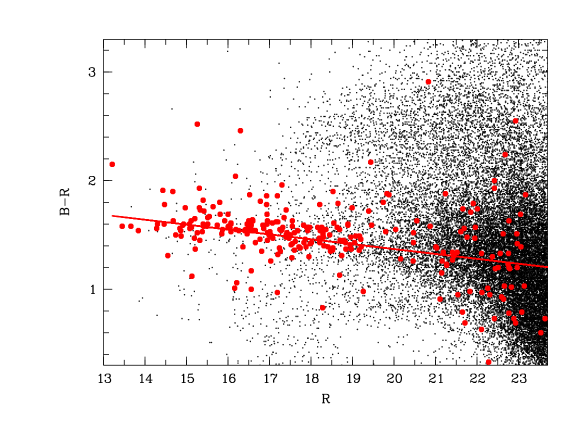
Figure 5: The color-magnitude diagram of galaxies. Spectroscopically confirmed members of the cluster (Coma in this specific case) are indicated with red circles, while black dots represent galaxies along the line-of-sight. Clusters contain unusual concentrations of bright galaxies which look more redder than most field galaxies. These galaxies exhibit a tight correlation between their colors and magnitudes. The narrow horizontal line of galaxies at nearly constant color is referred to as the elliptical ridge. Astronomers look for this characteristic shape in the color-magnitude diagram to select cluster members against foreground and background galaxies. (Taken from adami2 .)

Another important characteristic of clusters is that they are closed systems. In other words, they tend to hold their gas, unlike galaxies, where the gas is forced out through, for example, supernova explosions. X-ray studies have revealed the presence of large amounts of this intra-cluster gas which contributes to nearly $\sim 15\%$ of the total mass of the system. Since it is very hot, with temperatures in between 10⁷K and 10⁸K, this plasma emits X-rays in the form of thermal bremsstrahlung and makes clusters the brightest X-ray sources after Active Galactic Nuclei (see Fig. 6). The total mass of the diffuse intra-cluster gas is larger than that condensed in its galaxy members by roughly a factor of three (e.g. marhu even if this is still not enough mass to keep the galaxies in the cluster!) In particular, since clusters are closed systems, by assuming that their gas mass fraction is universal, one can estimate the total mass density of the universe.

The inner physical properties and the dynamical evolution of bound clusters is a major subject of scientific investigation. Nonetheless, also their large scale spatial distribution is a statistics of great cosmological interest. The space density of rich clusters is of order $10^{-5}$ Mpc^-3 so that the typical distance between cluster centers, if they were uniformly distributed in space, would be of order $\sim 50$ Mpc. These figures can be compared with the space density of mean galaxies ($10^{-2}$ Mpc^-3) and their typical separations ($\sim 5$ Mpc). Contrary to initial expectations (Nymann and Scott 1952) NYS clusters themselves are not uniformly distributed but are strongly correlated in space on scales nearly 5 times larger than those of galaxies.

By measuring the spatial abundance of clusters and its time evolution, one can constrain the growth rate of large-scale structures, thereby placing further significant constraints on the coherence of our standard cosmological model and on the viability of alternative theories of gravity. This motivate the search for high redshift systems, an extremely challenging task due to the fact that at such early epochs clusters are rare and projection effects hamper their identification.

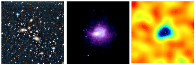
Figure 6: The cluster Abell 1914 as detected in different wave-bands. In the optical, a galaxy cluster is simply a cluster of galaxies, shown as the structure in the center of the figure on the left. In X-rays, a galaxy cluster is a glowing ball of electrons, emitting by thermal bremsstrahlung, with most of the baryons (the ordinary matter) in the form of hot ionized gas between the galaxies (center, courtesy of Bonamente). At radio-mm wavelengths, the same hot gas shows up as a shadow in the Cosmic Microwave Background (CMB), by a mechanism known as the Sunyaev-Zel’dovich effect. Effectively, the hot electrons give a small energy boost to the CMB photons as the photons go through the cluster, leading to a distortion of the spectrum of the CMB (Courtesy of J. Carlstrom)

3 Identification and reconstruction methods

From a physical point of view, a group or cluster of galaxies can be defined as a gravitationally bound system having a negative total mechanical energy (evaluated in the center of mass). This requirement (virial equilibrium) when coupled with the geometric constraint of sphericity implies that bound clusters must have an adimensional overdensity $\delta\rho/\langle\rho\rangle$ with respect to the background mass density field $\langle\rho\rangle$ of nearly 200.

From an astronomical point of view, identifying clusters in terms of these dynamical requirements turns out to be problematic. The overdensity criterium is only a necessary condition. It does not guarantee that systems satisfying to it are virialized. In particular the threshold sets a constraint on the overall distribution of matter in real space, not on the density contrast of the visible fraction in redshift space, i.e. the quantity which is directly accessible by observations. Additionally, only three of the seven parameters (3D-positions, 3D-velocities and masses) necessary to evaluate the energy of the system are actually observables. These are the angular (sky) position of galaxies and their redshift, i.e. their distance from the observer.

As we will see, one can bypass the incomplete knowledge of the coordinates needed to identify a cluster in phase space, by introducing some additional hypotheses concerning the symmetries of the system or the physical properties of its members. For example, it is fairly intuitive to characterize clusters as large and symmetrical conglomerates, the rich and poor categories being essentially defined by the number of red galaxies located within a given distance of the order of a few Megaparsec from the center of the system (see Fig. 6). In essence, one aims at identifying overdensities in redshift space, luminosity and/or color space, depending on the availability of redshift information and/or photometry. It is clear, that the degree of objectiveness of the cluster identification algorithm fully rests on the robustness of these external, model-dependent, constraints.

Given the limited number of observables and the large uncertainties with which they are estimated, one might think the identification of bound structures to be quite hopeless. It is not. The situation is saved by the statistical nature of the problem. Since clusters contains many members and there are many clusters in the universe, one can find in the theory of statistics the useful theorems and tools to average out reconstruction errors and imperfections.

With this caveat in mind, the ideal group-finding algorithm would be a single method that can robustly identify and determine the membership of groups and clusters of galaxies across a wide range of richness, mass, redshift and surveys sampling rate. (As an example galaxy structures may range from $\sim 10^{13}M_{\odot}$ to $\sim 10^{15}M_{\odot}$ in mass and are expected to densely populate the universe even at such early epochs as $z=1.5$). Additionally, the algorithm should impose minimal constraints on the physical properties of the clusters, to avoid selection biases. If not, these biases must be properly characterized.

The optimally reconstructed catalog of groups ought to fulfill two criteria: first it should be complete, in the sense that all the objects which fulfill the selection criteria are contained in the catalogue. Second it should be reliable i.e. it should not contain any object that do not fulfill the selection criteria (the so-called false positives). More specifically, the algorithm should be able to produce a catalog in which (1) all galaxies that belong to real groups are identified as group members, (2) no field galaxies are misidentified as group members, (3) all reconstructed groups are embedded within real, virialized dark-matter halos, (4) all real groups are identified as distinct objects ger .

3.1 Finding galaxy systems in 2D

Obtaining spectral information (distance measurements) is extremely demanding in terms of instrumental complexity and observing time. Therefore, it is critical to develop efficient group searching strategies able to detect intrinsically three-dimensional clusters in bi-dimensional data such as photographic plates, CCD images, catalogs of angular positions of the galaxies, etc (see top panel of figure 7).

One of the most enduring legacies George Abell has left to astronomy is the northern sky catalog of galaxy systems that he compiled in the 1950’sabel . By means of a visual inspection (and the aid of a $3.5x$ magnifying lens) Abell surveyed the then recently completed Palomar Sky Survey photographic plates, and identified 2,712 density excess in the galaxy distributions.

According to his identification algorithm, a cluster is a compact structure with fifty or more members lying within one “counting radius” of the cluster’s center (now called the Abell radius). Additionally, he divided the clusters into six “richness” groups, depending on the number of galaxies in a given cluster that lie within the magnitude range $m_{3}$ to $m_{3+2}$ (where $m_{3}$ is the magnitude of the third brightest member of the density excess).

The Abell cluster catalog is by far the most widely used catalog to date in the local universe. However, this ground breaking work has not stood the test of time as a valuable and efficient way for evaluating galaxy systems. Although the human eye is a sophisticated and efficient detector for galaxy clusters, it suffers from subjectivity and incompleteness, and visual inspection is extremely time consuming. Above all, the whole procedure is suitable only for rich clusters and does not apply to less massive systems characterized by a lower density contrast with respect to the background of unrelated objects. For cosmological studies, the major disadvantage of such visually constructed catalogs is that it is difficult to quantify selection biases. In this sense the Abell catalogue is neither complete nor is it reliable.

Only in recent years it has become possible to use numerical algorithms in the search for galaxy clusters in wide field optical imaging surveys. These modern studies required that photographic plates be digitized (so that the data are in machine readable form) or that the data be digital in origin, coming from CCD cameras gal .

Counts in cells method

Shectman (She ) was the first to use an automated method to search for clusters in 2D catalogs. His box-counting technique is based on identifying local density maxima above a threshold value, after smoothing data with a weighted kernel. This algorithm uses sliding windows which are moved across the point (galaxy) distribution marking the positions where the count rate in the central part of the window exceeds the value expected from the background determined in the outermost regions of the window.

However kernel smoothing invariably reduces the amount of information that can be retrieved from data. In this type of algorithms, for example, the kernel is fixed in angular size and, as a consequence, it does not smooth clusters at different distances with the same efficiency, making its sensitivity highly redshift dependent. The main drawbacks of the method are the introduction of a binning to determine the local background, which improves count statistics at the expense of spatial accuracy.

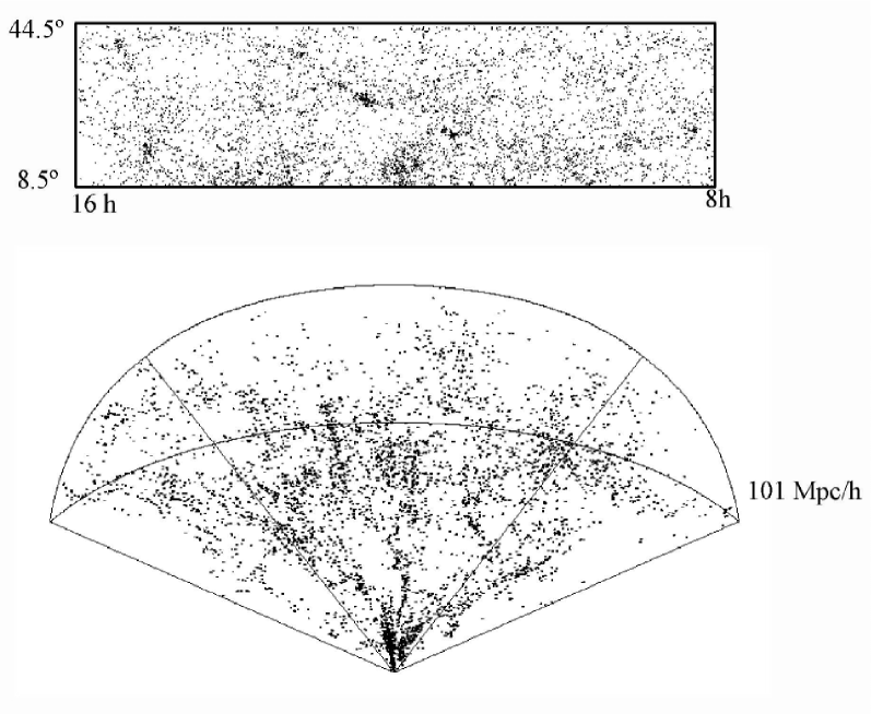
Figure 7: top: 2D map of the galaxy distribution in a flux-limited survey. Galaxy positions are specified using angular coordinates. Clusters are easily recognized in this sky map as galaxy overdensities on an otherwise smooth background. A difficult task is to get rid of fore- and back-ground objects which do not belong to clusters, or to identify weaker peaks usually associated to poor or distant clusters (only the most luminous members of which show up in a flux-limited galaxy survey) Bottom: the same galaxy distribution is shown in 3D space. Galaxy distances are inferred by interpreting the redshift, i.e. the relative shift of light wavelengths between emission and absorption, as due to the cosmological expansion of space. The redshift, which is an intrinsically kinematic observable, is also sensitive to non-cosmological Doppler contributions. Because of this spurious contamination (which is induced by the local motions of galaxies inside the gravitational potential well of a cluster) galaxies belonging to a gravitationally bound structure such as clusters appear smeared out along the observer line of sight in 3D maps, the so-called ”Fingers-of-God” phenomenon. (Courtesy of V. Martinez)

.

A slightly more sophisticated technique is to use an adaptive smoothing kernel sil . Even the introduction of locally adjustable searching parameters, however, does not significantly improve the performances of the technique when it is applied to galaxy catalogs spanning a wide range of depths. Moreover, cluster richness is evaluated in a step separate from detection, which further complicates the implementation of the method.

The matched filter technique

A substantial improvement in efficiency in finding clusters in two-dimensional optical data was obtained with the ‘matched filter’ technique of Postman et al. (post ). This technique, widely used in telecommunication (where it is known as the North filter) consists in correlating a known signal (or template), with an unknown signal to detect the presence of the template in the noisy background.

Postman et al. analyzed the galaxy distribution by adopting an a-priori cluster model to fit the data. In particular, by assuming a specific cluster radial density profile and a cluster luminosity function they constructed a matched filter in position and magnitude space. In practice, the 2D sky image is convolved with the assumed cluster model; all structures that resemble the filter will be filtered as little as possible, but structures that are different will get attenuated. This method, therefore, converts a 2D sky image into a 2D likelihood map. The intensity of the resulting map approximate the probability of each point being the center of a cluster.

Postman et al. realized that using magnitudes, rather than simply searching for spatial density enhancements, suppresses false detections that occur by chance projection. The matched filter is a very powerful cluster detection technique. It can handle deep surveys spanning a large redshift range, and provides redshift and richness measures as an innate part of the procedure. However, the main drawback of the method is that clusters which have properties inconsistent with the input functions will be detected at lower likelihood, if at all. In particular it can miss clusters that are not symmetric or whose density distribution differ significantly from the model profile. Therefore this algorithm does not performs optimally over large redshift baselines where a-priori unknown evolutionary effects are expected to modify significantly the simple representations used as input in the local universe (see the discussion by Gal ). Nevertheless, this remains one of the best cluster detection techniques for cluster detection in moderately deep surveys.

Photometric techniques

Systematic searches for clusters using galaxies as signposts for detection are mostly based on identifying a class of special objects supposed to live preferentially in high density environments.

One approach consists in looking for clusters directly in the sky. The strategy is to assume that luminous Active Galactic Nuclei (AGN) are found preferentially in high density regions. This is actually expected in models of galaxy formation. If the redshift of the AGN is known, one can use opportunely selected narrow-band filters to survey the regions around the AGN in quest of possible neighbors. In other words, by using a purely photometric technique one looks for the existence of a density excess of objects at the same distance of the AGN.

Another approach exploits the fact that late-type galaxies are the dominant population in the field, whereas early-types are preferentially seen in high-density regions (see Fig. 4). Therefore, any technique that can eliminate field (i.e., late-type) galaxies on the basis of some simple observable parameter will enhance the contrast of galaxy clusters relative to the background. For example, a popular algorithm uses the color-magnitude relation as a filter (see Fig. 5) to select possible cluster members (the Red Sequence method YGL ).

The implementation of these methods requires that images of the same sky region be available in two different optical bands. In particular since, the elliptical ridge (red sequence) is such a strong indicator of a cluster’s presence, this technique can be used to detect clusters to high redshifts ($z\sim 1$) with comparatively shallow imaging, if an optimal set of photometric bands is chosen. Moreover the redshift evolution of the red cluster sequence is so precisely characterized, that from the color-magnitude diagram of a cluster alone, its redshift can be estimated, whereby a typical accuracy of $dz\sim 0.1$ is achieved.

While using a color-magnitude relation to identify possible cluster members could enhance the identification success rate, it is also likely to suffer from selection biases, such as missing systems with significant blue populations of galaxies, namely, the Butcher-Oemler (BO ) clusters. As a consequence, one should not overlook the possibility that the resulting catalogs do not provide a complete census of the cluster population.

Recent methods have been developed to minimize the impact of these selection biases. For example the MaxBCG han ; koe or the K2 than methods are specifically designed and tailored to detect galaxy clusters in multicolor images. These identification algorithms look for ‘distinctive signatures’ such as the simultaneous galaxy density enhancements in both colors and position spaces, as well as the eventual presence of a bright galaxy in the targeted region.

Another class of methods is intermediate between 2D and 3D cluster finders. For example, Adami et al. 2010 adami3 used an adaptive kernel technique to reconstruct density maxima from photometric redshifts (i.e. redshifts estimated on the basis of galaxy colors as opposed to galaxy spectra). This approach has the drawback of being “data demanding”, in that it requires a multi passband 2D survey in at least 5 photometric bands. Nonetheless, at variance with purely 2D methods, the method opens up the possibility of searching for very distant ($z>1$) clusters.

Non-optical techniques

The various searching strategies we have described try to eliminate some of the subjective criteria and assumptions of past attemps, particularly detection by eye. Notwithstanding, a common problem of all these algorithms is that the recovered cluster samples are statistically complete only near the upper tail of the mass distribution. In effect, these methods identify only those rich aggregates that are most conspicuous. However, less extreme systems such as galaxy groups, which contain most of the luminosity, and presumably mass, of the universe, may be more useful probes of the large-scale structure. Additionally, in the absence of information about galaxy distances, projection effects are a serious and difficult to quantify issue. In photometric surveys, the increased depth necessary for high-redshift studies increases the overall number density of objects, thereby increasing the problems of foreground and background contamination and projection effects (although photometric techniques for estimating redshifts can mitigate these difficulties).

Since identification biases, essentially due to foreground and background contamination, plague any optically selected cluster sample (and have often translated into flawed scientific conclusions) alternative approaches to identify clusters in 2D have been investigated: X-ray emission from hot intra-cluster gas ros ; pierre ; fino , strong lensing induced by the cluster gravitational potential kneib2003 ; limousin2009 ; richard2010 , cosmic shear due to weak gravitational lensing ref ; gavazzi2009 , the Sunyaev-Zel’dovich (SZ) effect in the cosmic microwave background car ; voit . However, most of the methods used for local studies have only limited effectiveness at high redshift. The apparent surface brightness of X-ray clusters dims as $(1+z)^{-4}$, making only the richest clusters visible at high redshift. The cross section for gravitational lensing falls rapidly at high redshifts, making weak-lensing detection of distant clusters difficult for all but the most massive objects. The SZ effect is very promising, since it is entirely independent of redshift, but it also suffers from confusion limits and projection effects, and, in any case, large surveys of SZ clusters, such as those promised by the South Pole Telescope Staniszewski or the Planck satellite bartlett , are yet in a preliminary stage.

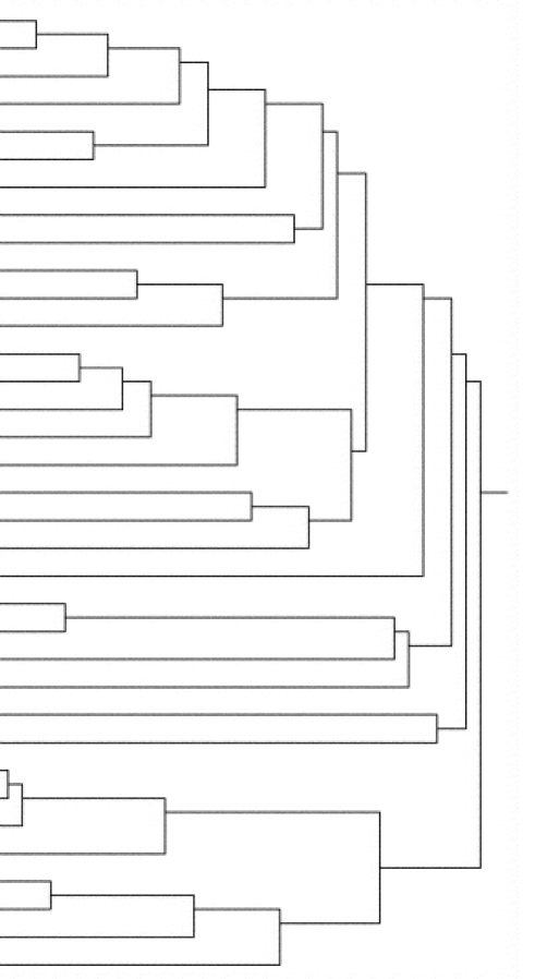
Figure 8: Dendogram showing how a set of galaxies merge and form a hierarchy. One starts with all galaxies of the sample as separate units and links the units successively in order of decreasing affinity until there is only one unit that encompasses the ensemble. The vertical axis measures the decreasing strength of the affinity parameter according to which galaxies are linked The limiting value of the affinity parameter below which one define clustered and isolated units must be fixed using independent physical considerations (Taken from gaz .)

3.2 Finding galaxy systems in 3D

The first sizeable sample of groups detected in redshift space was presented in 1983 by Geller & Huchra GH , who found 176 groups of three or more galaxies in the CfA galaxy redshift survey at redshifts $z<0.03$. Recently, Yang et al. yang identified groups within the 4th data release of the Sloan Digital Sky Survey (SDSS). Their catalog extends to $z<0.25$ covers one tenth of the sky and constitutes the largest currently available catalog of galaxy groups, containing $\sim 3\cdot 10^{5}$ groups with two or more members.

Despite the additional dimension, identifying in an unbiased way groups and clusters in redshift space is a formidable task. The most obvious and well-known complication is redshift-space distortions: the orbital motions of galaxies in virialized groups cause the observed group members to appear spread out along the line of sight (the Fingers-of-God effect), while coherent infall of outside galaxies into existing groups and clusters reduces their separation from group centers in the redshift direction (the Kaiser effect kaiser ). Both of these effects confuse group membership by intermingling group members with other nearby galaxies (see Fig. 7).

Since it is impossible to separate the peculiar velocity field from the Hubble flow without an absolute distance measure dek ; mari98 , this confusion can never be fully overcome, and it will be a significant source of error in any group-finding program in redshift space.

A second complication arises from incomplete sampling of the galaxy population. No modern galaxy redshift survey can succeed in measuring a redshift for every target galaxy, and an incomplete galaxy sampling rate always leads to errors in the reconstructed catalog of groups and clusters even without redshift-space distortions.

Moreover, surveys conducted over a broad redshift range present their own impediments to group finding. The major problem is that distant galaxies appear fainter than nearby galaxies. At high redshift one can probe only relatively rare, luminous galaxies, so only a small fraction of a given group’s members will meet a given selection criteria.

The hierarchical method

In the astronomical community the most widely used objective 3D group-finding algorithms are the hierarchical and the percolation (friends-of-friends) algorithms. In the hierarchical clustering method, first introduced by Materne (Mat ), one defines an affinity parameter between the galaxies, which controls the grouping operation. There are several possible choices for the grouping parameter. The most widely adopted choice is to use the product of galaxy luminosities divided by separation squared, which is a proxy of the gravitational force between galaxies i and j. Then one starts with all galaxies of the sample as separate units and links the galaxies successively in order of decreasing affinity until there is only one unit that encompasses the ensemble. A hierarchical sequence of units organized by decreasing affinity is the result of this method. The merging of a galaxy into a given unit involves the consideration of the whole unit and not just of the last object merged into the unit. Another merit of this method is the easy visualization of the whole merging procedure under the form of a hierarchical arborescence, the dendrogram (see Fig. 8).

Customarily, it is believed that the Hierarchical method has the practical drawback of requiring a very long calculation time (e.g., in comparison with the percolation method). Paying attention to this problem, Giuricin et al. (giu ) have managed to considerably speed up the hierarchical code by using numerical tricks. In this way, one can run this code nearly as fast as the percolation algorithm. For example the C programming language allows to use techniques of sparse matrix (i.e., with most elements equal to zero) in a natural way, through a data structure based on pointers. In this way, for each pair of galaxies, the affinity parameter, is not stored in memory and is not exactly calculated but replaced with zero if its value is smaller than a preselected limit. The maximum value of this parameter is searched only for the few pairs for which the parameter values are greater than this limit. Then the limit is gradually lowered in the following steps until the dendrogram is completed.

The main drawback of this procedure is that the threshold value where one cuts the hierarchy and below which one accepts the clusters as real is not supplied by the method, and must be fixed arbitrarily. A common choice is to cut the hierarchy according to the luminosity density or number density of the unity. This is a parameter which is highly sensitive to redshift distortions (see Fig. 7). In particular rich structures can have very low apparent densities in redshift space because their members are scattered away along the line-of-sight by the cluster potential. Clearly by lowering the density selection threshold, one could in principle recover these real structures but at the price of contaminating the catalog with lots of spurious, artificial structures.

The percolation method

The percolation or friends-of-friends (FOF) algorithm HG , being easier to implement than the Hierarchical one, has been the most widely used method of group identification in 3D. Moreover, since this technique has a natural theoretical motivation in the context of current model of galaxy formation, it has been extensively applied to detect overdensities not only in redshift surveys but also in N-body simulations of the large scale structure.

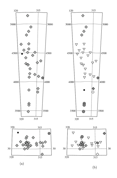
Figure 9: Comparison of the performances of the FOF and Hierarchical methods in identifying cluster members in high density regions. Galaxies in the region of the Abell 3574 clusters are shown in projection along the line-of-sight (upper panels) and on the sky (lower panels). Similar symbols are use to label galaxies identified as members of the same group by the percolation method (left panel) and the hierarchical method (right panel) (Taken from mari .)

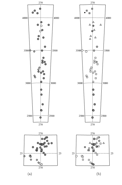
Figure 10: Same as in Fig. 9 but in the region of the the Hydra overdensity (Taken from mari .)

Unlike the Hierarchical algorithm, this technique does not rely on any a-priori assumption about the geometrical shape of groups. All pairs linked by a common “friend” form a group if the number overdensity contrast exceed an arbitrarily fixed critical threshold $\delta n/n$.

We here present more in detail the FOF algorithm adopted by Eke et al. eke . Consider two galaxies $i$ and $j$ with comoving distances from the observer $d_{i}$ and $d_{j}$ respectively. These two galaxies are assigned to the same group if their angular separation $\varphi_{ij}$ satisfies

$$\varphi_{ij}\leq\frac{1}{2}\left(\frac{r_{\perp,i}}{d_{i}}+\frac{r_{\perp,j}}{d_{j}}\right)$$ (2)

and, simultaneously, the difference between their distances satisfies

$$\left|d_{i}-d_{j}\right|\leq\frac{r_{\parallel,i}+r_{\parallel,j}}{2}.$$ (3)

where $r_{\perp}$ and $r_{\parallel}$ are the comoving linking lengths perpendicular and parallel to the line of sight. In order to take into account the decrease of the magnitude range of the luminosity function sampled at increasing distance in flux limited surveys, the projected link parameter, $r_{\perp}$ and $r_{\parallel}$ are in general suitably increased with increasing distance. By scaling them, one keeps the number density enhancement $\delta n/\langle n\rangle$ constant. However, the scaling prescriptions, besides being somewhat arbitrary, introduces serious biases in the reconstructed group catalog. Eke et al. adopted the following scheme

$$r_{\perp} = \min\left[r_{\rm max}(1+z),\frac{b}{\langle n\rangle}^{1/3}\right]$$ (4)

$$r_{\parallel} = R\;r_{\perp},$$ (5)

arguing that scaling both $r_{\perp}$ and $r_{\parallel}$ with $\langle n\rangle^{-1/3}$ will compensate for the magnitude limit and lead to groups of similar shape and overdensity throughout the survey.

The FOF algorithm has three free parameters: the linking length $b$, the maximum perpendicular linking length in physical coordinates $r_{\rm max}$, and the ratio between the linking length along and perpendicular to the line of sight $R$. The free parameter $r_{\rm max}$ has been introduced to avoid unphysically large values for $r_{\perp}$ at high redshifts where the galaxy distribution is sampled very sparsely. Since $r_{\rm max}$ is measured in physical coordinates, $r_{\rm max}(1+z)$ is the maximal comoving linking length perpendicular to the line of sight. The free parameter $R$ allows $r_{\parallel}$ to be larger than $r_{\perp}$ taking into account the elongation of groups along the line of sight due to the Fingers-of-God effect. Finally, the linking parameter $b$ can be constrained, in real space, by modelling a cluster as a bound structure resulting from the non-linear gravitational collapse of a spherical perturbation. Because of this, the percolation algorithm is a natural method for identifying virialized structures in the absence of redshift-space distortions and is largely used to recover groups and clusters in real-space N-Body numerical simulations.

In figures 9 and 10 two characteristic high density regions (Abell 3574 and Hydra clusters) of the universe are shown together with the cluster identified by two different group-finding algorithms: the FOF and Hierarchical methods. By inspecting them one can qualitatively contrast the performances of these two methods. The hierarchical algorithm, selecting preferentially systems with a spherical symmetry, fails to recover massive clusters with prominent Fingers of God, whose members are better identified using the percolation algorithm.

These standard cluster-finding algorithms are less than optimal for many reasons. For instance, the searching window at the heart of FOF techniques is insensitive to local variations in the density of points. Assigned cluster membership therefore depends on the scale of the adopted linking length and not the distribution of galaxies alone, violating the dictum to ”let the data speak for themselves”. In fact, both the hierarchical and the percolation methods require prior knowledge and/or user-fixed parameters to produce their best results. Density thresholds, linking-length parameter scaling laws, galaxy selection functions, etc., must all be set in advance. The preprocessing and/or trial-and-error tests required to tune these algorithms for a particular data set are extremely inefficient and may even lead to systematic differences among different applications of the same technique.

It is well known that the performance of the standard FOF algorithm across a wide range of density enhancements is not uniform. A generous linking length is preferred in studies that aim to identify high velocity dispersion systems. On the other hand, studies of loose associations require short velocity links, but this can result in a bias toward low velocity dispersion measurements. In general, the velocity dispersion of systems identified with the FOF algorithm is $\sim 30\%$ higher than the velocity dispersion of groups identified in the same galaxy catalog by the hierarchical method (giu ). To further complicate matters, clusters identified with one method may not be detected by the other.

Given the weaknesses/failings of traditional cluster identification methods, which are likely to only be worse at high redshift (a domain which is progressively conquered by modern observational campaigns), there have been various attempt to explore new detection strategies. Kepner et al. (kepner ) generalized in 3D the matched filter algorithm. This new adaptive code identifies clusters by adding halos to a synthesized background mass density and computing the maximum-likelihood mass density. The Sloan Digital Sky Survey team has introduced a group-finding algorithm called C4 (nichol ), which searches for clustered galaxies in a seven-dimensional space, including the usual three redshift-space dimensions and four photometric colors, on the principle that galaxy clusters should contain a population of galaxies with similar observed colors. In quest of the optimal algorithm, various researchers have also explored the possibility of using the geometries of Voronoi and Delaunay.

4 Voronoi based group-finding tools

The Voronoi tessellation made his “debut” in cosmology as an useful theoretical framework for interpreting the clustering of galaxies (IW ; WI ) . Since then, it has been used as a valuable method for investigating several issues concerning the large-scale structure of the universe (see phdvw and the review of Van de Weygaert in this volume.)

The Voronoi partition of a space into minimally sized convex polytopes – the three-dimensional analogue of Dirichlet tessellation or determination of Thiessen polygons – provides a natural way to find cluster centers (peaks in the galaxy density field). The volume inside each polyhedron is inversely proportional to the packing efficiency of its seed; a large cell volume indicates that its seed is comparatively isolated. While other methods estimate the galaxy density field by smoothing the distribution of data points with an a priori physical model, window profile or binning strategy, the Voronoi diagram provides a density estimator that is asymptotically local: the density measured at a position ${\bf x}$ is determined completely by the positions of the neighboring data points, while the influence of distant points vanishes.

The Delaunay complex, the simultaneously-determined dual of the Voronoi diagram, implicitly contains vast amounts of proximity information. It yields a natural measurement of inter-galaxy scale lengths while remaining linearly proportional in size to the dataset. By providing a natural linking structure for a set of objects, the Delaunay triangulation allows to reconstruct the members of a galaxy cluster.

Figure 11: Bidimensional Voronoi tessellation of the distribution of galaxies in a particular sky region. Each triangle represents a galaxy surrounded by its associated Voronoi cell (indicated by the polyhedrals). The area of this cell is interpreted as the effective area a galaxy occupies in the plane. The inverse of this area gives the local density at that point. Galaxy clusters are identified by high density regions, composed of small adjacent cells, i.e. , cells small enough to give a density value higher than the chosen density threshold (Taken from ram .)

In what follows I give an overview of various Voronoi-based group-finding methods that have been developed in an astronomical context. I will first present algorithms that have been conceived for cluster identification in 2D imaging surveys. Then, I will discuss in greater detail the Voronoi-Delaunay Method (VDM) proposed by Marinoni et al. (mio ) for identifying structures in 3D redshift surveys.

4.1 2D Voronoi algorithms

Brown (1965) and Ord (1978) were the first to suggest the use of Voronoi cell volumes as density measures. The algorithm of Ebeling & Wiedenmann (ew ), in particular, was the first Voronoi based peak finder method in the astronomical literature. It was introduced as an optimal way to detect overdensities in X-ray photon counters and thus identify astronomical X-ray sources. Since then, Voronoi based density estimators have rapidly grown in popularity (and sophistication) and have been applied to investigate a large class of astronomical phenomena (see Schaap00 ; scha ; WeySchaap09 ).

Ebeling & Wiedenmann partitioned the detector surface using 2D Voronoi cells and defined as overdensity regions those composed by adjacent Voronoi cells with a density higher than the chosen threshold. They used a rigorous statistical approach for setting the detection criteria. An empirical distribution function describing randomly positioned points following Poissonian statistics, has been proposed by Kiang (k ):

$$dp(\tilde{a})=\frac{4^{4}}{\Gamma(4)}\tilde{a}^{3}e^{-4\tilde{a}}d\tilde{a},$$ (6)

where $\tilde{a}\equiv a/\langle a\rangle$ is the cell area in units of the average cell area $\langle a\rangle$. The idea of Ebeling & Wiedenmann was to estimate the background noise by fitting the Kiang cumulative distribution to the empirical cumulative distribution resulting from the data points in the region of low density which is not affected by the presence of structures ($\tilde{\rho}\equiv\rho/\langle f\rangle\,\leq 0.8$). In this way they were able to minimize the contamination of spurious detections.

This algorithm can be used quite generally to find any kind of structures embedded in a noisy background field. Ramella et al (ram ) in particular used it to identify galaxy clusters in bi-dimensional sky images as significant density fluctuations above the background (see Fig. 11). They noted that the procedure, being completely non-parametric, is particularly sensitive to both symmetric and elongated and/or irregular clusters. Sampling of the density distribution is just the first step in a cluster detection procedure, followed by location of the density peaks that fulfil the criteria for a galaxy cluster The simplest approach is to select objects with a certain contrast above the background. Notwithstanding, the choice of the appropriate threshold is not trivial. With increasing threshold, the detection rate of the real clusters is declining, but also the relative number of spurious clusters detected is dropping. Moreover, in the outer regions of the clusters, where the number density is gradually dropping, the detection of the member galaxies is strongly dependent on the assumed threshold. Because of this, more refined methods, instead of sharp density thresholds, use a Maximum Likelihood techniques to increase the identification efficiency and better delineate the boundaries of the Voronoi selected clusters in 2D (see method and discussion by soc ).

The false/positive detection rate is hard, if not impossible, to quantify, without running an algorithm on a catalog with extensive spectroscopy. Anyway, one can compare the relative performances of different cluster-finding codes by running them on the same 2D photometric catalog. By running their Voronoi Galaxy Cluster Finder (VGCF) on the same data (the Palomar Distant Cluster Survey (PDCS)) processed by Postman et al. with their matched filter method, Ramella et al. were able to identify 37 clusters. Of these clusters, 12 are VGCF counterparts of the 13 PDCS clusters detected at the 3$\sigma$ level. Of the remaining 25 systems, 2 are PDCS clusters with confidence level $<3\sigma$. According to Ramella et al. inspection of the 23 new VGCF clusters indicates that several of these clusters may have been missed by the matched filter algorithm for one or more of the following reasons: a) they are very poor, b) they are extremely elongated, c) they lie too close to a rich and/or low redshift cluster.

Figure 12: Top: Example of Voronoi tessellation executed on the galaxy distribution around Abell cluster 957. Each cell encloses one galaxy. The data presented here has a lower boundary in declination, which is why the Voronoi tessellation seems to diverge below. The filled circles mark galaxies satisfying the selection criteria, $\delta(\bar{a}-a)/\bar{a}\rangle 3$ where $a$ is the area of a Voronoi cell and $\bar{a}$ its average value. No significant overdensity of the filled circles around Abell 957 appears when using the entire distribution of galaxies. Bottom: same as above but the Voronoi tessellation is evaluated only on the galaxies that satisfy the color-magnitude criteria used in the VTT. Unlike above the cluster is now strikingly enhanced by the filled circles, which denote galaxies with $\delta>3$. (Taken from kim .)

An upgraded version of a Voronoi based algorithm to identify galaxy clusters in 2D images was proposed by Kim et al. (kim ). In order to increase the detection performance, their recipe for the Voronoi Tessellation Technique (VTT) uses a-priori knowledge of some characteristics of the cluster member galaxies, namely, the characteristic ridge in the color-magnitude diagram (see Fig. 5). By applying a filter in color-magnitude space they reduce the contamination of projection effects and greatly enhance the cluster members contrast relative to the background.

Once the color-magnitude diagram has been used to preselect potential cluster members Kim et al. apply the Voronoi tessellation on the resulting distribution of galaxies and select only cells whose area satisfy an empirically defined boundary condition. In practice, potential candidates are identified by requiring a minimum number N of galaxies having overdensities $\delta$ greater than some threshold $\delta_{c}$, within a radius of fixed size. The top panel of figure 12 shows Voronoi tessellation executed on all galaxies in the region of Abell 957, whereas the bottom one shows only those galaxies that satisfy the color-magnitude cut. One can immediately appreciate the remarkable enhancement of the cluster, with respect to the previous case.

By using simulations to compare their algorithm against a matched-filter method, they found that the matched-filter algorithm outperforms the VTT when using a background that is uniform, but it is more sensitive to the presence of a nonuniform galaxy background than is the VTT. This last method has also a better overall false-positive rate compared with the MF.

Lopes et al. (lopes ) applied both the VGCF and the adaptive kernel techniques to identify clusters over the 2700 square degrees of the digitized Second Palomar Observatory Sky Survey (DPOSS). The comparison of catalogs generated by these different techniques is not a straightforward task. As they underline, even clusters that are identified by various techniques might have large differences in the measurement of properties such as richness, or projected density profiles. Notwithstanding, by contrasting both algorithms they find that the Voronoi algorithm performs better for poor, nearby clusters, while the adaptive kernel goes deeper and detects richer systems. Anyway, they conclude that in order to obtain more complete and unbiased cluster catalogs it is imperative to minimize contamination by random fluctuations in the galaxy distribution and chance alignments of galaxy groups by complementing geometrical tools with multicolor photometric information such as the color-magnitude diagram.

In this spirit, Van Breukelen et al. (van ) developed an hybrid cluster-finding algorithm based on a combination of the Voronoi tessellation on 2D images and Friends-Of-Friends methods applied to photometric estimates of the galaxy redshift. They use Montecarlo simulations to assign a reliability factor F to each cluster and then cross-correlate the cluster candidates output by the Voronoi and FOF methods by taking all cluster candidates that are detected in both with F greater then a fixed threshold.

A common feature of all the previous algorithms which make use of the Voronoi partition to identify cluster candidates in 2D, is that cluster members identification is usually carried out using additional and independent methods. For example, the most popular technique consists in selecting as clusters members those galaxies which lie within fixed-radius spheres centered on the Voronoi-detected peaks or use the percolation algorithm. In the following, I will describe a 3D technique in which this last reconstruction step is consistently carried out using the dual structure of a Voronoi partition, i.e. the Delaunay tessellation.

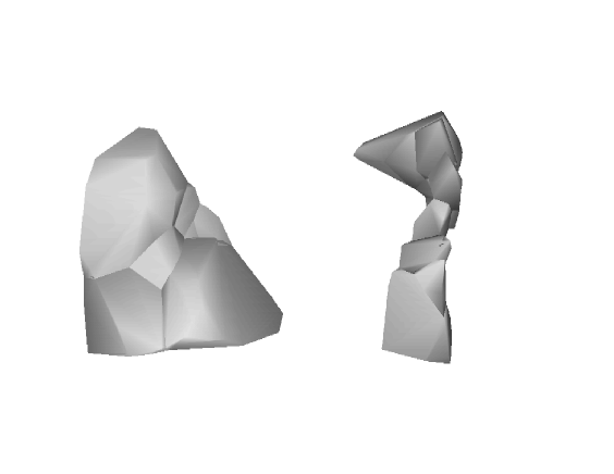
Figure 13: Three-dimensional Voronoi reconstruction of a cluster with 10 galaxies in a galaxy simulation. The Voronoi cells encompassing each cluster galaxy are shown in real space (bottom) and in redshift space (top). Each Voronoi 3D cell surrounding a galaxy is defined as the intersection of the planes which are perpendicular bisectors of the lines joining that galaxy to its neighbors. Note how the nearly isotropic real-space distribution of cluster galaxies degenerates into a composite Voronoi structure which is elongated along the observer’s line of sight.

4.2 The 3D Voronoi and Delaunay Method

The Voronoi-Delaunay Method we developed (VDM, mio ) makes use of the Voronoi partition and Delaunay triangulation to identify and reconstruct galaxy clusters in 3D redshift surveys (see Fig. 13). Once the Voronoi/Delaunay calculation for a 3D catalog of galaxies has been completed, the algorithm proceeds in three phases. First, peaks in density (obtained by sorting the inverse volumes into a monotonic sequence) are identified and provide candidate locations for cluster centers. The Delaunay mesh then allows to identify central members of each candidate group and estimate physical properties such as the cluster central density. Finally, these estimates are used to define redshift space windows within which we find each group’s members. In this last step it is the predicted structure of the clusters, inferred from an initial level of grouping, that influences local decisions regarding galaxy membership.

Figure 14: Top: simplified 2-dimensional graphic representation of phase I of the VDM algorithm. Sky angular coordinates are along the x axis, and the survey depth is displayed along the y axis. Dots represent individual galaxies, while the shaded area represents the Voronoi cell surrounding a possible cluster seed (represented by an asterisk). The set formed by the asterisk and the points marked with triangles represents the first order Delaunay neighbors. Bottom Simplified 2-dimensional graphic representation of phase II (§3.2.2). Sky angular coordinates are along the x axis, and the survey depth is displayed along the y axis. Segments represent the Delaunay mesh connecting the galaxy distribution shown in the top panel. First-order Delaunay neighbors are represented by triangles and second-order Delaunay neighbors by diamonds. Note that not all the galaxies inside the search window (shaded area) are used to define the projected central density parameter $N_{II}$, but only those designated by symbols. (Taken from mio .)

Phase I: Finding systems of galaxies

We begin by assuming that the centers of clusters will lie near peaks in the galaxy density field. To identify these peaks, we sort all the galaxies in the catalog by the inverse volume of their Voronoi cell; the smallest cells are most likely to fall at density maxima and are thus potential “seeds” for finding groups or clusters. We must next determine if a given seed actually lies at the heart of a system of galaxies.

Each cluster seed is linked to its nearest neighbors by the Delaunay mesh. We are interested only in real, physical groupings of galaxies; we therefore must define some ad hoc threshold in an attempt to distinguish galaxies that could be physically bound together from galaxies which are in chance proximity to each other. We consider to be neighbors those Delaunay-connected points whose distance from the seed galaxy is less than a fixed limit ${\cal R}_{min}$. These galaxies, and the original seed galaxy itself, will be referred to hereafter as first-order Delaunay neighbors and are used to determine the system’s center of mass.

If no galaxies satisfy this criterion then the cluster seed will be rejected and considered an isolated galaxy. If, when analyzing a seed we find that all its first-order Delaunay neighbors have already been assigned to another structure, we automatically merge the seed galaxy into that system. A schematic representation of this first step in cluster identification is presented in the top panel of Fig. 14.

Because there is a fairly tight correlation between cluster richness and the order in which they are reconstructed (as we proceed from the highest density cells to the lowest, the richest clusters are generally identified first), we need not test every object as a potential cluster center. Instead, in the interest of computational speed we exclude the cells around galaxies that have already been assigned to systems from being themselves considered as other cluster seeds or members. We thus proceed through the catalog in order of increasing Voronoi cell volume, identifying every object in the clusters through the three-phase process described above and then moving to the next smallest Voronoi cell as yet unclustered, until the entire catalog has been either assigned to a cluster or tested as a potential cluster seed.

Phase II: Determining clustering strength

Since they are calculated in a parameter-free fashion, both the Voronoi diagram and Delaunay complex are determined isotropically in the angular and redshift directions. However, the peculiar velocities induced by a cluster’s gravitational field cause the distribution of galaxies to appear elongated in the redshift direction to a degree determined by its velocity dispersion. The three-dimensional information lost in the transformation to redshift space cannot be recovered uniquely via isotropic, geometric methods; additional assumptions are required to minimize contamination by spurious members. To determine the properties of clusters with any accuracy, we require methods that include this anisotropy.

We therefore define a cylindrical window in redshift space (centered on the barycenter determined in Phase I and circular in the angular dimensions) within which we may find objects which are very likely to be members of each cluster. This cylinder will have radius ${\cal R}_{II}\geq{\cal R}_{min}$ and length (along the redshift direction) ${\cal L}_{II}$. We define those galaxies which fall within this cylinder and are connected to first-order Delaunay neighbors by the Delaunay mesh as second-order Delaunay neighbors; see the bottom panel of Fig. 14 for a graphical illustration. Note that not all the galaxies in the cylinder are included.

We set ${\cal R}_{II}={\cal R}_{min}=1^{-1}$Mpc comoving, which is the typical central radius theoretically predicted for massive and virialized clusters. Analogous physical considerations guide us to set the half-length of the cylindrical window, ${\cal L}_{II}$, to be $20h^{-1}$Mpc. This value includes the maximum line-of-sight peculiar velocity of galaxies that are identified as members of systems in N-body simulations (as high as $\sim 1500km/s$).

We then use the sum of the numbers of first- and second-order Delaunay neighbors as an indicator of the central richness of the group, $N_{II}$. By including only Delaunay neighbors in $N_{II}$, we are able to minimize contamination by interlopers, providing a robust estimate even in low-density systems. This is particularly important because $N_{II}$ controls the adaptive window for cluster members used in Phase III.

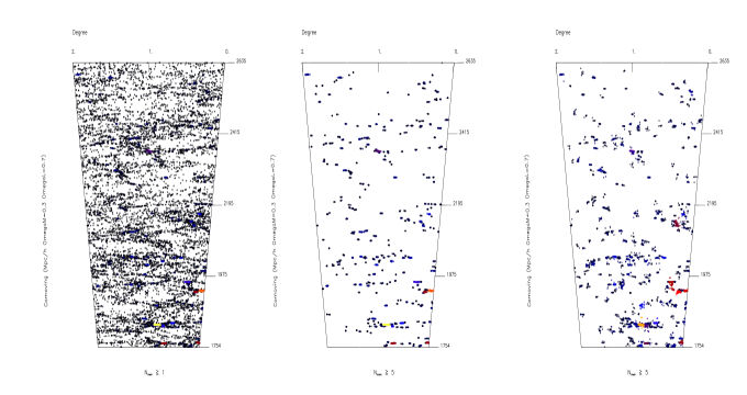
Figure 15: Left: N-body simulation of galaxies represented in a 2D, real-space cone diagram. The volume corresponds to an angular area of 1 square deg and to the redshift interval z=0.7-1.2 (here expressed in Mpc units). Center: real space, large-scale spatial distribution of galaxies belonging to clusters with more than 5 members as identified in the simulation. Right: real space, large-scale spatial distribution of galaxies belonging to clusters with more than 5 members as reconstructed by the VDM algorithm applied in redshift space. (Taken from mio .)

Phase III: Assigning cluster members

Having identified the center and estimated the central richness for each cluster, we then reconstruct the full set of system members. We do this on the basis of physical considerations, not via an empirically tuned parameter threshold. In particular, we exploit the known richness-velocity dispersion correlation to define a search window for each cluster’s members based upon its richness.

The virial theorem predicts that velocity dispersion and central number density of galaxies are correlated. bah observationally confirmed the existence of a strong linear correlation valid from loose groups to clusters. We rely on this relation to estimate the strength of the underlying clustering, which we then use to determine on a group by group basis the window around the system’s center within which to search for Delaunay-connected galaxies. Thus, the algorithm relies on the principle that cluster reconstruction should not proceed by linking a chain of ”friends” that could lead to any given galaxy in the sample, but instead should iterate the search for cluster members from a potential cluster center position outward in an adaptive fashion.

Specifically, for each cluster we define a cylindrical window (symmetric about the redshift direction) with radius ${\cal R}_{\rm II}$ and length $2{\cal L}_{\rm II}$ determined by the richness scale factor $N_{II}$ as follows

$${\cal R}_{\rm III} = r(\tilde{N}_{\rm II})^{1/3}$$ (7)

$${\cal L}_{\rm III} = l(\tilde{N}_{\rm II})^{1/3}f(z)$$ (8)

whereas $r$ and $l$ are two free parameters, $\tilde{N}_{\rm II}$ is the central richness corrected for the redshift dependent mean density $\langle n\rangle(z)$, and $f(z)$ is a function introduced to take into account that for a fixed velocity dispersion the length of the fingers of god in redshift space is a function of redshift. $\tilde{N}_{\rm II}$ and $f(z)$ are given (in an arbitrary cosmology of matter density $\Omega_{m}$ and vacuum energy density $\Omega_{\Lambda}$) by

$$\tilde{N}_{\rm II}=\frac{\langle n\rangle(z_{\rm ref})}{\langle n\rangle(z)}N_{\rm II}$$ (9)

and

$$f(z)=\frac{s(z)}{s(z_{\rm ref})},\ \ \ s(z)=\frac{1+z}{\sqrt{\Omega_{m}(1+z)^{3}+\Omega_{\Lambda}}}$$ (10)

respectively, where $z_{\rm ref}$ is an arbitrary reference redshift.

By using the Delaunay mesh to identify the nearby galaxies, we are able to reconstruct group membership quite rapidly; once the initial Voronoi-Delaunay calculation is complete (which need only be done once for a catalog), it takes only 1 minutes on a modern workstation to process $\sim 15000$ galaxies into a catalog of groups and clusters.

Tests of the VDM algorithm

What is more important, and what is not usually done for other methods, the performances of the algorithm have been tested using N-body simulations of deep redshift surveys. This allows a quantitative characterization of the completeness of the resulting group catalog.

In particular Gerke et al. (ger ) found that the group-finder can successfully identify $\sim 78\%$ of real groups and that $\sim 79\%$ of the galaxies that are true members of groups can be identified as such. Conversely, $\sim 55\%$ of the groups found can be definitively identified with real groups and $\sim 46\%$ of the galaxies placed into groups are interloper field galaxies.

To give a visual sense of the errors encountered in reconstructing individual groups, we show several examples of group-finding success and failure in figures 15 and 16.

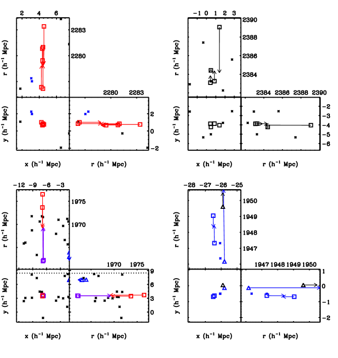
Figure 16: Examples of group-finding success and failure ger . In each panel, squares indicate galaxies in a simulated group being plotted, triangles indicate galaxies in nearby real groups, and crosses indicate nearby field galaxies. Galaxies are plotted both as seen on the sky and in two line-of-sight projections in redshift space. Arrows point to the galaxies real space positions, to show the effects of redshift-space distortions (to reduce visual clutter, no arrows are plotted for field galaxies). Dotted lines indicate field edges. Each reconstructed group is indicated by a different shade, with reconstructed field galaxies shown in black. The top left panel shows a perfect reconstruction with a nearby false detection; the top right panel shows a completely undetected group (all black squares), the bottom left panel shows a fragmented real group, and the bottom right panel shows an example of over-merging. (Taken from ger .)

A compared analysis of the VDM and FOF performances has also been carried out knoebel and the main result is graphically summarized in figure 17 where the performances of the two methods in recovering a particular structure are contrasted. This structure is probably an example of a “super-group”, where several smaller groups are just about to merge fino .

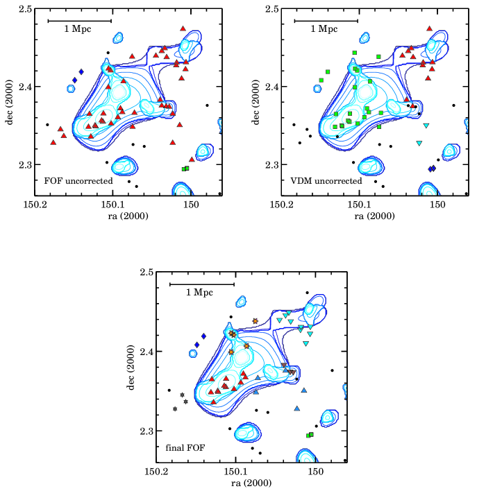
Figure 17: The upper left panel shows the structure as reconstructed by the FOF method, the upper right the VDM recovered systems. Because of the failure of the FOF, the group recovered by this method has been a-posteriori manually split up into several groups (lower panel). Black points denote field galaxies, and the other symbols (squares, triangles, etc.) are group galaxies, whereas each group has its own symbol and color. The blue contour exhibit the X-ray emission of the super-group as observed with XMM-Newton. Taken from knoebel .

The upper left panel shows the group assignment of the FOF method, and the upper right panel the group assignment of the VDM. Each group is denoted by a symbol (e.g. square, triangle) of a particular color, and field galaxies by black points. This example of the super-group gives us some interesting insights concerning the group-finding procedure.

This extended structure exhibits the main potential problems of both the FOF and VDM algorithms. The FOF algorithm connected practically all the galaxies in this super-group, without distinguishing between different sub-groups. As discussed, this behavior is well known for FOF, and it happens in particularly dense regions such as this. The problem is that any single galaxy between two of these sub-clusters will act as a bridge for the FOF algorithm to connect the two clusters. The VDM is more successful in distinguishing different sub-structures, but nevertheless fails to do a perfect job. A casual glance suggests that the “green square” VDM cluster in fact consists of two independent sub-groups (consistent with the X-ray contours). Furthermore, the “red triangle” VDM group exhibits two outliers to the South which almost certainly do not belong to this group. The occurrence of such outliers is not uncommon in VDM groups. It is related to the fact that in the VDM group-finder every second order Delaunay-neighbor in the second cylinder is accepted as group member and that the second cylinder is usually much bigger than the third cylinder knoebel .

Since, as we have seen, any group-finding algorithm is prone to many different types of systematics, it is crucial to define carefully the tolerance for various errors and craft a specific definition of group-finding success. We focused our efforts on reproducing as accurately as possible only those specific group properties which are more relevant for cosmological purposes. In particular Marinoni et al. and Gerke et al. showed that it is possible to quantify the completeness of the resulting group catalog. directly in the physical space of velocity dispersions. In other words, it is possible to define a velocity dispersion threshold $\sigma$ above which a critical cosmological statistics such as the spatial abundance of systems at a given redshift ($N(>\sigma,z)$) is recovered in a complete way with a sufficient degree of accuracy.

A common feature of most of the algorithms which make use of the Voronoi partition to identify cluster candidates in 2D, is that cluster members identification is usually carried out using additional and independent methods. For example, the most popular technique consists in selecting as clusters members those galaxies which lie within fixed-radius spheres centered on the Voronoi-detected peaks or use the percolation algorithm. On the contrary in the 3D VDM technique this last reconstruction step is consistently carried out using the dual structure of a Voronoi partition, i.e. the Delaunay tessellation. This offers the possibility of adaptively scaling cluster selection window only on the basis of the geometrical characteristics of the Voronoi and Delaunay meshes, i.e. on the basis of completely non-parametric structures.

I will emphasize three other aspects of the VDM algorithm. a) The method is based on the specific idea that cluster reconstruction does not proceed by linking potential friends to any given galaxy in the sample (such as in the standard 3D percolation or hierarchical methods), but by iterating the search of cluster members from a potential cluster center position outward (which is the natural identification process in visual or 2D cluster reconstruction);
b) there is no need to introduce an arbitrarily chosen global density threshold to judge when a given system is formed. Instead the cluster searching window is locally scaled on a cluster by cluster basis using physical arguments (in the specific case the strength of the first Delaunay connected units);

5 Conclusions

The VDM algorithm, working with controlled reliability and completeness over a wide range of redshifts and a large degree of density enhancements, has been used to identify groups and clusters in all the existing deep redshift surveys of the universe: the DEEP2 ger , the VVDS cucciati , and the zCOSMOS knoebel surveys.

Ongoing analysis, however, shows that, despite remarkable progresses, we have yet to design the ”perfect” group-finder. While recovering rich systems is quite straightforward (especially in redshift surveys), reconstructing with high efficiency structures with fewer members (i.e. poor groups or poorly sampled clusters) is technically challenging. In particular, the level of completeness and purity with which groups are currently identified ($\sim 80\%$) is still far from optimal.

A temporary way out consists in compensating for weaknesses and failures characterizing each single method by cross-identifying and matching structures in catalogues produced by different algorithms knoebel . Anyway, developing more sophisticated cluster finding algorithms is crucial if we want to reconstruct galaxy environment with high precision and use the next generation of deep 3D data to answer key cosmological questions.

It is also critical to stress that the optical identification of a strong spatial concentration of galaxies is not a sufficient criterium for the identification of a virialized cluster of galaxies. It is by no means clear whether, in this way, one has found a gravitationally bound and relaxed system of galaxies and the corresponding dark matter halo. Even centrally condensed structures, as far as the optical distribution of galaxies is concerned, may show relevant substructures in the diffuse gas distribution when their X-ray image is analyzed. For example, the Coma cluster, long considered to be a regular cluster, is not completely in an equilibrium state, but it is dynamically evolving presumably by the accretion of an adjacent galaxy group.

With this caveat in mind, it is encouraging to turn the head backward and appraise the long way walked from the very early days dominated by a sort of skeptical attitude towards this cosmographical endeavor up to an epoch, the present, in which we can reliably use catalogs of optical groups an clusters to gain access to a wealth of crucial cosmological information.

- (1) W. A. Baum et al: ApJ, 130, 749 (1959)
- (2) W. de Sitter: Proc. Acad. Sci., 19, 1217 (1917)
- (3) E. Hubble: Proceedings of the National Academy of Sciences 15, 168 (1929)
- (4) C. Charlier: Ark. Mat. Astron. Fys., 16, 1 (1922)
- (5) J. L. E. Dreyer: New General Catalogue of Nebulae and Clusters of Stars. Mem. Roy. Astron. Soc. 49, Part I (reprinted 1953, London: Royal Astronomical Society).
- (6) J. L. E. Dreyer: Index Catalogue of Nebulae Found in the Years 1888 to 1894, with Notes and Corrections to the New General Catalogue. Mem. Roy. Astron. Soc. 51, 185 (reprinted 1953, London: Royal Astronomical Society).
- (7) J. L. E. Dreyer: Second Index Catalogue of Nebulae Found in the Years 1895 to 1907. Mem. Roy. Astron. Soc. 59, Part 2, 105 (reprinted 1953, London: Royal Astronomical Society)
- (8) C. Adami, A. Biviano, F. Durret & A. Mazure: A&A, 443, 17 (2005)
- (9) G. O. Abell: ApJS, 3, 211 (1958)
- (10) H. K. C. Yee, M. D. Gladders: Astronomical Journal, 120, 2148 (1999),
- (11) A. Dressler: ApJ, 236, 351 (1980)
- (12) S-M. Niemi, P. Nurmi, P. Heinamaki & M. Valtonen: MNRAS, 382, 1864 (2007)
- (13) N. Bahcall: in Formation of Structure in the Universe. Ed. A. Dekel and J. P. Ostriker. Cambridge: Cambridge University Press, p.135
- (14) A. Biviano: in Constructing the Universe with Clusters of Galaxies, IAP 2000 meeting, Paris, France, July 2000, Florence Durret & Daniel Gerbal Eds. (arXiv:astro-ph/0010409)
- (15) A. Mercurio et al: A&A, 397, 431 (2003)
- (16) C. Adami et al: A&A, 507, 1225 (2009)
- (17) C. Marinoni & M. Hudson: ApJ, 569, 101 (2002)
- (18) J. Neyman & E. L. Scott: ApJ, 116, 144 (1952)
- (19) F. Zwicky: Helvetica Physica Acta, 6, 110 (1933)
- (20) P. Rosati et al: ARA&A, 40, 539 (2002)
- (21) M. Pierre et al: MNRAS, 372, 591 (2006)
- (22) A. Finoguenov et al: ApJS, 172, 182 (2007)
- (23) J.-P. Kneib et al: ApJ, 598, 804 (2003)
- (24) M. Limousin et al: A&A, 502, 445 (2009)
- (25) J. Richard et al: MNRAS, 404, 325 (2010)
- (26) A. Refregier: ARA&A, 41, 645 (2003)
- (27) R. Gavazzi et al: A&A, 498, 33 (2009)
- (28) J. E. Carlstrom et al: ARA&A, 40 643 (2002)
- (29) G. M. Voit: Review of Modern Physics, 77, 207 (2005)
- (30) Z. Staniszewski et al: ApJ, 701, 32 (2009)
- (31) J. G. Bartlett et al: Astronomische Nachrichten, 329, 147 (2007)
- (32) R. R. Gal, arXiv:astro-ph/0601195 (2006)
- (33) S. A. Shectman: ApJS, 57, 77 (1985)
- (34) B. W. Silverman: Monographs on Statistics and Applied Probability, London: Chapman and Hall (1986)
- (35) M. Postman et al: AJ, 111, 615 (1996)
- (36) R. Gal: Lecture Notes in Physics, 740, 119 (2008)
- (37) H. Butcher & A. Oemler: ApJ 285, 426 (1984)
- (38) S. M. Hansen et al: ApJ, 633, 122 (2005)
- (39) B. P. Koester et al: ApJ, 660, 239 (2007)
- (40) K. Thanjavur et al: ApJ, 706, 571 (2009)
- (41) C. Adami et al: 2010, A&A 509, 81
- (42) M. J. Geller & J. P. Huchra: ApJS, 52, 61 (1983)
- (43) X. Yang et al: ApJ, 671, 153 (2007)
- (44) N. Kaiser: MNRAS, 227, 1 (1987)
- (45) A. Dekel: ARA&A, 32, 371 (1993)
- (46) C. Marinoni et al: ApJ, 505, 484 (1998)
- (47) J. Materne: A&A, 63, 401 (1978)
- (48) J. P. Huchra & M. J. Geller: ApJ, 257, 423 (1982)
- (49) V. R. Eke et al: MNRAS, 248, 866 (2004)
- (50) G. Giuricin et al: ApJ, 543, 178 (2000)
- (51) J. Kepner et al: ApJ, 517, 78 (1999)
- (52) C. J. Miller et al: ApJ, 130, 968 (2005)
- (53) N. Ghazzali et al: ApJ, 511, 242 (1999)
- (54) C. Marinoni et al: ApJ, 580, 122 (2002)
- (55) C. Marinoni: The nearby universe: cosmography, cosmogony, and cosmology PHD Thesis, University of Trieste (2002)
- (56) V. Icke & R. van de Weygaert: A&A, 184, 16 (1987)
- (57) R. van de Weygaert & V. Icke: A&A, 213, 1 (1989)
- (58) A. Okabe, B. Boots & K. Sugihara: Spatial tessellations: concepts and applications of Voronoi diagrams. New York: Wiley & Sons (1992)
- (59) R. Van de Weygaert: Ph.D. thesis, Leiden University (1991)
- (60) G. S. Brown: New Zealand Forestry Service Research Notes 38, 1 (1965)
- (61) J. K. Ord: Math. Scientist, 3, 23 (1978)
- (62) M. Ramella et al: A&A, 368, 776 (2001)
- (63) H. Ebeling & G. Wiedenmann: Phys. Rev. E, 47, 704 (1993)
- (64) W. E. Schaap & R. van de Weygaert: A&A, 363, L29 (2000)
- (65) W. E. Schaap: PhD Thesis, Rijksuniversiteit Groningen, The Netherlands (2007)
- (66) R. van de Weygaert & W. E. Schaap: The Cosmic Web: Geometric Analysis. In: Data Analysis in Cosmology, eds. V. Martínez et al., Lecture Notes Phys., 665, 291-413 (Springer-Verlag) arXiv:0708:1441
- (67) T. Kiang 1966: Zeitschrift fur Astrophysik, 64, 433 (1966)
- (68) I. Sochting, R. G. Clowes & L. E. Campusano: MNRAS, 347, 1241 (2004)
- (69) R. S. J. Kim et al: AJ, 123, 20 (2002)
- (70) P. A. A. Lopes et al: AJ, 128, 1017 (2004)
- (71) C. Van Breukelen et al: MNRAS, 373, 26 (2006)
- (72) N. A. Bahcal: ApJ, 247, 787 (1981)
- (73) B. Gerke et al: ApJ, 625, 6 (2005)
- (74) C. Knoebel et al: ApJ, 697, 1842 (2009)
- (75) O. Cucciati et al: A&A, 520, 42 (2010)