Scalar-isoscalar states, gravitational form factors, and dimension-2 condensates in a large-$N_{c}$ Regge approach

Abstract

Scalar-isoscalar states ($J^{PC}=0^{++}$) are analyzed within the large-$N_{c}$ Regge approach. We find that the lightest $f_{0}(600)$ scalar-isoscalar state fits very well into the pattern of the radial Regge trajectory. We confirm the obtained mass values from an analysis of the pion and nucleon spin-0 gravitational form factors, recently measured on the lattice. We find that a simple two-state model suggests a meson nature of $f_{0}(600)$, and a glueball nature of $f_{0}(980)$, which naturally explains the ratios of various coupling constants. Finally, matching to the OPE requires a fine-tuned mass condition of the vanishing dimension-2 condensate in the Regge approach with infinitely many scalar-isoscalar states.

1 Introduction

Hadron resonances appearing in the PDG tables increase their mass while their width remains constant Amsler et al. (2008). On the other hand, in the large-$N_{c}$ limit, with $g^{2}N_{c}$ fixed, mesons and glueballs are stable, their masses become independent on $N_{c}$, $m={\cal O}(N_{c}^{0})$, while their widths $\Gamma$ are suppressed as $1/N_{c}$ and $1/N_{c}^{2}$, respectively, which means that $\Gamma/m$ is suppressed (see e.g. Pich (2002) for a review). This suggests that excited states in the mesonic spectrum may follow a reliable large-$N_{c}$ pattern. The main feature of a resonance is that it corresponds to a mass distribution, with values approximately spanning the $m\pm\Gamma/2$ mass interval. The lowest resonance in QCD is the $0^{++}$ state $f_{0}(600)$ or the $\sigma-$meson, which appears as a complex pole in the second Riemann sheet of the $\pi\pi$ scattering amplitude at $s_{\sigma}=m_{\sigma}^{2}-im_{\sigma}\Gamma_{\sigma}$ with $m_{\sigma}=347(17){\rm MeV}$ and $\Gamma_{\sigma}/2=345(24){\rm MeV}$ Caprini et al. (2006) (see also Ref. Kaminski et al. (2008)). Higher $0^{++}$ states are listed in Table 1.

For scalar states a measure of the spectrum is given in terms of the trace of the energy momentum tensor Donoghue and Leutwyler (1991)

$$\Theta^{\mu}_{\mu}\equiv\Theta=\frac{\beta(\alpha)}{2\alpha}G^{\mu\nu a}G_{\mu\nu}^{a}+\sum_{q}m_{q}\left[1+\gamma_{m}(\alpha)\right]\bar{q}q.$$ (1)

Here $\beta(\alpha)=\mu^{2}d\alpha/d\mu^{2}$ denotes the beta function, $\alpha=g^{2}/(4\pi)$ is the running coupling constant, $\gamma_{m}(\alpha)=d\log m/d\log\mu^{2}$ is the anomalous dimension of the current quark mass $m_{q}$, and $G_{\mu\nu}^{a}$ is the field strength tensor of the gluon field. This operator connects scalar states to the vacuum through the matrix element

$$\langle 0|\Theta|n\rangle=m_{n}^{2}f_{n}.$$ (2)

The two-point correlator reads

$$\Pi_{\Theta\Theta}(q)=i\int d^{4}xe^{iq\cdot x}\langle 0|T\left\{\Theta(x)\Theta(0)\right\}|0\rangle$$ (3)

$$= \sum_{n}\frac{f_{n}^{2}q^{4}}{m_{n}^{2}-q^{2}}=q^{4}\left[C_{0}\log q^{2}+\sum_{n}\frac{C_{2n}}{q^{2n}}\right],$$

where in the second line we saturate with scalar states and the large $q^{2}\gg\Lambda_{\rm QCD}$ limit is taken. Comparison with the Operator Product Expansion (OPE) Narison (1998) leads to

$$C_{0} = -\lim_{n\to\infty}\,\frac{f_{n}^{2}}{dm_{n}^{2}/dn}=-\frac{N_{c}^{2}-1}{2\pi^{2}}\left(\frac{\beta(\alpha)}{\alpha}\right)^{2},$$ (4)

$$C_{2} = \sum_{n}f_{n}^{2}\qquad\qquad=0\,,$$ (5)

$$C_{4} = \sum_{n}f_{n}^{2}m_{n}^{2}\qquad\quad=\left(\frac{\beta(\alpha)}{\alpha}\right)^{2}\langle G^{2}\rangle\,.$$ (6)

Equation (4) requires infinitely many states, while Eq. (5) suggests a positive and non-vanishing gauge-invariant dimension-2 object, $C_{2}=i\int d^{4}xx^{2}\langle\Theta(x)\Theta\rangle$, which is generally non-local, as it should not appear in the OPE.

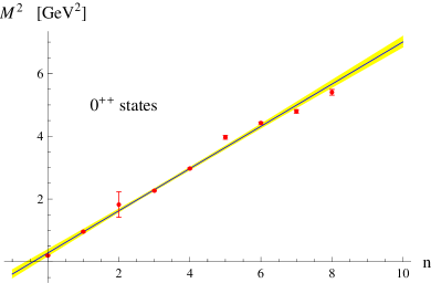
Figure 1: Radial Regge trajectory corresponding to the squared mass of all $J^{PC}=0^{++}$ scalar-isoscalar states listed in the PDG tables Amsler et al. (2008). The four heaviest $0^{++}$ states are not yet well established and are omitted from the PDG summary table. The error bars correspond to the errors in the determination of the square of mass, listed in Amsler et al. (2008). The straight line is the result of our fit.

2 Scalar Regge spectrum

Radial and rotational Regge trajectories were analyzed in Ref. Anisovich et al. (2000). In Ref. Anisovich (2006) the scalar sector was studied in more detail. Two parallel radial trajectories could then be identified, including three states per trajectory. In a recent work Ruiz Arriola and Broniowski (2010) we have analyzed all the $0^{++}$ states which appear in the PDG tables (see Fig. 1) and found that all fit into a single radial Regge trajectory of the form

$$M_{S}(n)^{2}=\frac{a}{2}n+m_{\sigma}^{2}.$$ (7)

The mass of the $\sigma$ state can be deduced from this trajectory as the mass of the lowest state. The resonance nature of these states suggests using the corresponding half-width as the mass uncertainty by minimizing

$$\chi^{2}=\sum_{n}\left(\frac{M_{f,n}-M_{S}(n)}{\Gamma_{f,n}/2}\right)^{2},$$ (8)

which yields $\chi^{2}/{\rm DOF}=0.12$ (see also Table 1) with

$$a=1.31(12){\rm~{}GeV}^{2},\quad\;m_{\sigma}=556(127){\rm~{}MeV}\,.$$ (9)

Formula (7) is equivalent to two parallel radial Regge trajectories with the standard slope

$$M_{S,-}(n)^{2} = a\,n+m_{\sigma}^{2},$$ (10)

$$M_{S,+}(n)^{2} = a\,n+m_{\sigma}^{2}+\frac{a}{2},$$ (11)

where $a=2\pi\sigma$, and $\sigma$ is the string tension associated to the potential $V(r)=\sigma r$ between heavy colored sources. The value $\sqrt{\sigma}=456(21)\,{\rm MeV}$ agrees well with lattice determinations of $\sqrt{\sigma}=420{\rm MeV}$ Kaczmarek and Zantow (2005).

This situation suggests the existence of a hidden symmetry in the $0^{++}$ sector. In the holographic approach based on the AdS/CFT correspondence the symmetry corresponds to parity in the fifth-dimensional variable. This is similar to the one-dimensional harmonic oscillator; all states with the energy $E_{n}=\hbar\omega(n+1/2)$ can be separated in parity even and odd states, with energies $E_{n}^{(+)}=2\hbar\omega(n+1/4)$ and $E_{n}^{(-)}=2\hbar\omega(n+3/4)$, respectively, having twice the slope of $E_{n}$.

Resonance	$M$ [MeV]	$\Gamma$ [MeV]	$n$	$M$ (Fit)
$f_{0}(600)$	$400-1200$	$500-1000$	0	$556$
$f_{0}(980)$	$980(10)$	$70(30)$	1	$983$
$f_{0}(1370)$	$1350(150)$	$400(100)$	2	$1274$
$f_{0}(1500)$	$1505(6)$	$109(7)$	3	$1510$
$f_{0}(1710)$	$1724(7)$	$137(8)$	4	$1714$
$f_{0}(2020)$	$1992(16)$	$442(60)$	5	$1896$
$f_{0}(2100)$	$2103(8)$	$209(19)$	6	$2062$
$f_{0}(2200)$	$2189(13)$	$238(50)$	7	$2215$
$f_{0}(2330)$	$2321(30)$	$223(30)$	8	$2359$

Table 1: PDG values of resonance parameters Amsler et al. (2008), compared to the fit to the radial Regge spectrum of the $0^{++}$ scalar-isoscalar states, $M_{n}^{2}=\frac{1}{2}an+m_{\sigma}^{2}$, given by Eq. (8). The lowest $n=0$ state, corresponding to the $f_{0}(600)$ resonance, is excluded from the fit.

Besides, there seems to be no obvious difference between mesons and glueballs, as far as the spectrum is concerned. Note that the Casimir scaling suggests that the string tension is $\sigma_{\rm glueball}=\frac{9}{4}\sigma_{\rm meson}$, but this holds in the case of fixed and heavy sources. The fact that we have light quarks might explain why we cannot allocate easily the Casimir scaling pattern in the light-quark scalar-isoscalar spectrum.

3 Gravitational form factors

Hadronic matrix elements of the energy-momentum tensor, the so-called gravitational form factors (GFF) of the pion and nucleon, correspond to a dominance of scalar states in the large-$N_{c}$ picture, as ($u(p)$ is a Dirac spinor)

$$\langle\pi(p^{\prime})|\Theta|\pi(p)\rangle = \sum_{n}\frac{g_{n\pi\pi}f_{n}q^{2}m_{n}^{2}}{m_{n}^{2}-q^{2}},$$ (12)

$$\langle N(p^{\prime})|\Theta|N(p)\rangle = \bar{u}(p^{\prime})u(p)\sum_{n}\frac{g_{nNN}f_{n}m_{n}^{2}}{m_{n}^{2}-q^{2}},$$ (13)

where the sum rules $\sum_{n}{g_{n\pi\pi}}{f_{n}}=1$ Narison and Veneziano (1989) $M_{N}=\sum_{n}g_{nNN}f_{n}$ Carruthers (1971) hold. Unfortunately, the lattice QCD data for the pion Brommel et al. (2007) and nucleon (LHPC  Hagler et al. (2008) and QCDSF Gockeler et al. (2004) collaborations), picking the valence quark contribution, are too noisy as to pin down the coupling of the excited scalar-isoscalar states to the energy-momentum tensor. Nevertheless, useful information confirming the (Regge) mass estimates for the $\sigma$-meson can be extracted using multiplicative QCD evolution of the GFF through the valence quark momentum fraction, $\langle x\rangle_{u+d}$, as seen in deep inelastic scattering or on the lattice at the scale $\mu=2{\rm GeV}$. For the pion GFF we obtain the fit

$$\langle x\rangle_{u+d}^{\pi}=0.52(2),\qquad m_{\sigma}=445(32){\rm~{}MeV}\,,$$ (14)

whereas for the nucleon GFF we get

$$\langle x\rangle_{u+d}^{N}=0.447(14),\qquad\ m_{\sigma}=550^{+180}_{-200}{\rm MeV}.$$ (15)

Assuming a simple dependence of $m_{\sigma}$ on $m_{\pi}$,

$$m_{\sigma}^{2}(m_{\pi})=m_{\sigma}^{2}+c\left(m_{\pi}^{2}-m_{\pi,{\rm phys}}^{2}\right),$$ (16)

yields $m_{\sigma}=550^{+180}_{-200}{\rm MeV}$ and $c=0.95^{+0.80}_{-0.75}$, or $\ m_{\sigma}=600^{+80}_{-100}{\rm MeV}$ and $c=0.8(2)$, depending on the lattice data Hagler et al. (2008) or Gockeler et al. (2004), respectively. Higher quark masses might possibly clarify whether or not the state evolves into a glueball or a meson, since in that case one has, respectively, either $m_{\sigma}/(2m_{q})\to 0$, or $m_{\sigma}/(2m_{q})\to 1$.

4 Dimension-2 condensates

It is interesting to discern the nature of the $\sigma$ state from an analysis of a truncated spectrum. The minimum number of states, allowed by certain sum rules and low energy theorems, is just two. In Ref. Ruiz Arriola and Broniowski (2010) we undertake such an analysis, which suggests that $f_{0}(600)$ (denoted as $\sigma$) is a $\bar{q}q$ meson, while $f_{0}(980)$ (denoted as $f_{0})$ is a glueball according to the $N_{c}$ scaling of various quantities (see Table 2). The argument is based on the fact that one obtains $f_{\sigma}/f_{f_{0}}\sim g_{f_{0}NN}/g_{\sigma NN}\sim g_{f_{0}\pi\pi}/g_{\sigma\pi\pi}\sim 1/\sqrt{3}$, however $C_{2}=f_{\sigma}^{2}+f_{f_{0}}^{2}\neq 0$ because the number of states is finite.

Table 2: $N_{c}$-scaling.

quantity	glueball	$q\bar{q}$ meson
$m_{n}$	1	1
$f_{n}$	$N_{c}$	$\sqrt{N_{c}}$
$\Gamma_{n\pi\pi}$	$1/{N_{c}^{2}}$	$1/N_{c}$
$g_{n\pi\pi}$	$1/N_{c}$	$1/\sqrt{N_{c}}$
$g_{nNN}$	$1$	$\sqrt{N_{c}}$

The infinite Regge spectrum of Eq.  (7) with Eq. (4) may be modeled with a constant $f_{f_{0}}=f_{n,+}={\cal O}(N_{c})$ discarding $f_{\sigma}=f_{n,-}={\cal O}(\sqrt{N_{c}})$ . Naively, we get $C_{2}=\infty$. However, $C_{2}$ may vanish, as required by standard OPE, when infinitely many states are considered after regularization. Using $\zeta$-function regularization Arriola and Broniowski (2007), yields Ruiz Arriola and Broniowski (2010)

$$C_{2}\equiv\lim_{s\to 0}\sum f_{n,+}^{2}M_{S,+}(n)^{2s}=f_{f_{0}}^{2}\left(1/2-m_{f_{0}}^{2}/a\right)\,,$$ (17)

which at leading $N_{c}$ implies $C_{2}=0$ for $m_{f_{0}}=\sqrt{a/2}=810(40){\rm MeV}$, a reasonable value to ${\cal O}(1/N_{c})$.

What should these $m_{\sigma}$ values be compared to? Besides the pole definition one also has the Breit-Wigner (BW) definition, which in the $\pi\pi$ data is disputed for the $\sigma$ but not for the $\rho$. Our analysis is driven by large-$N_{c}$ considerations (see also Refs. Pelaez and Rios (2009); Ruiz de Elvira et al. (2010)). In Ref. Nieves and Ruiz Arriola (2009) it was shown that the difference between the BW and the pole definitions is ${\cal O}(1/N_{c}^{2})$ and, further, that for $N_{c}=3$ the BW definition works as good for the $\sigma$ as for the $\rho$. In Ref. Nieves and Arriola (2009) it was argued that $m_{\sigma}-m_{\rho}={\cal O}(1/N_{c})$. Thus, we expect the present estimates to be in between, incorporating a systematic ${\cal O}(1/N_{c})$ mass shift.

References

• Amsler et al. (2008) C. Amsler, et al., Phys. Lett. B667, 1 (2008).
• Pich (2002) A. Pich (2002), hep-ph/0205030.
• Caprini et al. (2006) I. Caprini, G. Colangelo, and H. Leutwyler, Phys. Rev. Lett. 96, 132001 (2006), hep-ph/0512364.
• Kaminski et al. (2008) R. Kaminski, J. R. Pelaez, and F. J. Yndurain, Phys. Rev. D77, 054015 (2008), 0710.1150.
• Donoghue and Leutwyler (1991) J. F. Donoghue, and H. Leutwyler, Z. Phys. C52, 343–351 (1991).
• Narison (1998) S. Narison, Nucl. Phys. B509, 312–356 (1998).
• Anisovich et al. (2000) A. V. Anisovich, V. V. Anisovich, and A. V. Sarantsev, Phys. Rev. D62, 051502 (2000), hep-ph/0003113.
• Anisovich (2006) V. V. Anisovich, Int. J. Mod. Phys. A21, 3615–3640 (2006), hep-ph/0510409.
• Ruiz Arriola and Broniowski (2010) E. Ruiz Arriola, and W. Broniowski, Phys. Rev. D81, 054009 (2010), 1001.1636.
• Kaczmarek and Zantow (2005) O. Kaczmarek, and F. Zantow, Phys. Rev. D71, 114510 (2005), hep-lat/0503017.
• Narison and Veneziano (1989) S. Narison, and G. Veneziano, Int. J. Mod. Phys. A4, 2751 (1989).
• Carruthers (1971) P. Carruthers, Phys. Rept. 1, 1–29 (1971).
• Brommel et al. (2007) D. Brommel, et al. (2007), arXiv:0708.2249[hep-lat].
• Hagler et al. (2008) P. Hagler, et al., Phys. Rev. D77, 094502 (2008).
• Gockeler et al. (2004) M. Gockeler, et al., Phys. Rev. Lett. 92, 042002 (2004)
• Arriola and Broniowski (2007) E. R. Arriola, and W. Broniowski, Eur. Phys. J. A31, 739–741 (2007), hep-ph/0609266.
• Pelaez and Rios (2009) J. R. Pelaez, and G. Rios (2009), 0905.4689.
• Ruiz de Elvira et al. (2010) J. Ruiz de Elvira, J. R. Pelaez, M. R. Pennington, and D. J. Wilson (2010), 1009.6204.
• Nieves and Ruiz Arriola (2009) J. Nieves, and E. Ruiz Arriola, Phys. Lett. B679, 449–453 (2009), 0904.4590.
• Nieves and Arriola (2009) J. Nieves, and E. R. Arriola, Phys. Rev. D80, 045023 (2009), 0904.4344.