Autocorrelations in Hybrid Monte Carlo Simulations

Abstract:

Simulations of QCD suffer from severe critical slowing down towards the continuum limit. This problem is known to be prominent in the topological charge, however, all observables are affected to various degree by these slow modes in the Monte Carlo evolution. We investigate the slowing down in high statistics simulations and propose a new error analysis method, which gives a realistic estimate of the contribution of the slow modes to the errors.
CERN-PH-TH/2010-278
DESY 10-210
SFB/CPP-10-115

1 Introduction

Reliable estimation of physical quantities in lattice QCD requires that all possible sources of both systematic and statistical error are kept under control. In the continuum limit $a\to 0$ a severe slowing down of the topological charge has been observed [1]. Such slowing down corresponds to an increase in auto-correlation times beyond the naive scaling of the algorithm. This behavior is expected to influence not only the topological charge but also other observables and sets a limit on how close to the continuum we can get. However, given the need to simulate at increasingly finer lattice spacings in order to keep cut-off effects under control, it is of general interest to think about the consequences of analyzing data in presence of long auto-correlation times.

Our study starts from the observation that in a simulation different observables do have different auto-correlation times. The reason behind this is related to the spectral structure of the transition matrix that describes the stochastic evolution in Monte Carlo (MC) time. This observation can be used to formulate a procedure that gives conservative estimates of the statistical errors. The method we propose is about consistently using information from the slower sector of the simulation to give a safer estimate of the error of the mean value of observables that have shorter auto-correlation times.

2 Auto-correlations of Markov Chains

The error analysis of lattice QCD data has to deal with the presence of auto-correlations. This is a consequence of the fact that all known simulation methods belong to the class of Markov chain Monte Carlo (MCMC) algorithms. In the following we present a brief overview of the concepts and definitions used. For a more detailed summary and explanation we refer to [2] and references therein.

The auto-correlation function $\Gamma$ as a function of MC time $t$ is given by

$$\Gamma_{O}(t)=\lim_{N\to\infty}\;\frac{1}{N-t}\sum_{i=1}^{N-t}\,[\,O(q_{i+t})-\overline{O}\,]\,[\,O(q_{i})-\overline{O}\,]$$ (1)

where $N$ denotes the length of the MC history and $\overline{O}$ is the mean value of the observable $O$ as measured from the data. The integrated auto-correlation time is the integral of the auto-correlation function

$$\tau_{\mathrm{int}}(O)=\frac{1}{2}+\sum_{t=1}^{\infty}\rho_{O}(t)\;,\quad\text{where}\quad\rho_{O}(t)=\frac{\Gamma_{O}(t)}{\Gamma_{O}(0)}\;.$$ (2)

For a practical estimate, the sum in eq. 2 is in practice always truncated at some window $W$ (typically much smaller than $N$) whose size can be defined according to a criterion which balances the statistical and systematic uncertainties [3]. This naturally suffers from a truncation bias that is asymptotically removed as we increase the length of the total MC history and together move the truncation window towards larger times. For short histories in which the autocorrelation function itself is known with little precision, however, the truncation bias can be sizable. Since the integrated auto-correlation time enters the error formula for $\overline{O}$ as

$$\delta\overline{O}=\sqrt{\frac{2\tau_{\mathrm{int}}(O)\operatorname{var}{[O]}}{N}}\;,$$ (3)

a better estimator for $\tau_{\mathrm{int}}(O)$ would certainly lead to more reliable error bounds on the average of observables of interest.

By looking at the auto-correlation function of some observables shown in Fig. 1, all of them belonging to the same Markov chain, we can immediately see how some of them decay much faster than others. From the theory of Markov processes and some algorithmic considerations (for example the assumption that the algorithm has detailed balance) it is possible to derive the following spectral formula:

$$\Gamma_{O}(t)=\sum_{n\geq 1}(\lambda_{n})^{t}\;A_{n}(O)\,,\quad\text{where}\quad|\lambda_{n}|<1\quad\text{and}\quad A_{n}(O)\geq 0$$ (4)

where $\lambda_{n}$ are real eigenvalues of the Markov matrix, ordered as $\lambda_{1}\geq\lambda_{2}\geq\ldots\geq\lambda_{n}$ (again we refer to [2] for details on the derivation). From eq. 4 we can see that $\Gamma(t)$ is actually a linear combination of decaying exponentials with positive coefficients. An interpretation of Fig. 1 can then be given in terms of the amplitudes and the time constants $\tau_{n}=-1/\ln{\lambda_{n}}$ of the exponentials: observables with auto-correlation functions that decay more slowly have stronger coupling to the modes with larger time constant.

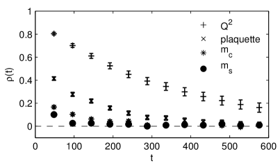
Figure 1: The normalized auto-correlation function for the HYP smeared topological charge squared, the smeared plaquette and the quenched pseudo-scalar mass of the $c\bar{c}^{\prime}$ and of the $s\bar{s}^{\prime}$ meson, computed respectively at the charm and at the strange quark mass. They are all computed at the same lattice spacing of $a\approx 0.074$fm.

From a real world Monte Carlo simulation it is virtually impossible to obtain a definite knowledge about the longest time constants involved. Since we need this information for the analysis, we therefore call $\tau_{*}$ our best estimate of the dominant time constant, which we can either take from a model or by investigating a large number of observables and take the largest observed value. Let us assume that for a given observable $O$ all relevant time scales are smaller (or of the same order) than the given $\tau_{*}$. If this is the case, we can choose a window $W_{u}$ (best at a time where the auto-correlation function is still significant), and define an upper bound to the estimator of the integrated auto-correlation time

$$\tau_{\mathrm{int}}^{u}(O)=\frac{1}{2}+\sum_{t=0}^{W_{u}}\rho_{O}(t)+A_{O}(W_{u})\tau_{*}\;,\quad\text{with}\quad A_{O}(W_{u})=\max\left(\rho_{O}(W_{u})\,,\,2\delta\rho_{O}(W_{u})\right)$$ (5)

where $\delta\rho_{O}$ denotes the error of the normalized auto-correlation function.

3 A case study: quenched pseudo-scalar meson mass

As a direct application of the ideas presented so far, we will examine in detail the case of the auto-correlation function of a quenched observable while critically applying to it the error formula in eq. 5. All the data we use is from a simulation with the Wilson gauge action at lattice spacing $a=0.075$fm and volume of $(2.4\text{fm})^{4}$. The algorithm used is the Domain Decomposed Hybrid Monte Carlo (DD-HMC) [5] reduced to the pure gauge action, with a block size of $16\times 8^{3}$. The size of our MC history is of 145000 Molecular Dynamics units (MDU, that we will use throughout the paper). The observables that we consider are quenched meson two-point functions, the plaquette and topological charge Q. In order to be more sensitive to the slow modes, we also compute some observables, in particular Q, on smoothed gauge fields. For this purpose we apply five levels of HYP smearing [4] to the link variables.

In order to apply eq. 5 we first need a value of the time constant $\tau_{*}$ used to compensate for truncating the tail contribution due to the slow modes. Our proposal here is to define an effective time constant $\tau_{\text{eff}}(t)$ by analogy with a QCD effective mass

$$\tau^{-1}_{\text{eff}}(t)=\log\left(\frac{\Gamma(t)}{\Gamma(t+\delta t)}\right)/\delta t\;,$$ (6)

where instead of computing it out of a two-point correlator we extract it from the auto-correlation function of the observable that has the best signal. The time $\tau_{*}$ can then be determined from a plateau average in an “effective mass” plot. This method will work well with observables that strongly couple to possibly a single (or a few very closely spaced) slow mode(s).

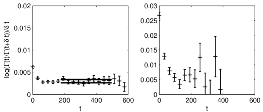
Figure 2: (Left) “Effective mass” plot for the auto-correlation function of the HYP smeared topological charge squared. (Right) Same plot for the smeared plaquette.

The slowest observable that we consider is the parity even $Q^{2}$ instead of the parity odd $Q$. The reason behind this choice is that even though in eq. 4 all modes contribute to $\Gamma$ for a given observable, if the integrator preserves a symmetry of the discretized action (in our case parity), it is possible to show that contributions come only from algorithmic modes in the same sector as the observable under study [2]. As shown in Fig. 2 this method is giving a very good plateau for the topological charge squared, while for the plaquette results are not as satisfactory. This has to do with the fact, already detectable in Fig. 1, that, in this particular case, the smeared plaquette couples more strongly to modes with time constant(s) $\tau_{n}$ smaller than the time scales determining the slow decay of $Q^{2}$. This does not mean that with $\tau_{*}$ we are identifying the slowest algorithmic mode (that would be $\tau_{1}$), but with it we are confident to have identified the slowest relevant mode for the error analysis of observables we are interested in. We obtain $\tau_{*}$ by averaging over the plateau shown in Fig. 2 and the value we measure is $\tau_{*}=330(45)$. This value can now be used to estimate the upper bound of the error of another observable.

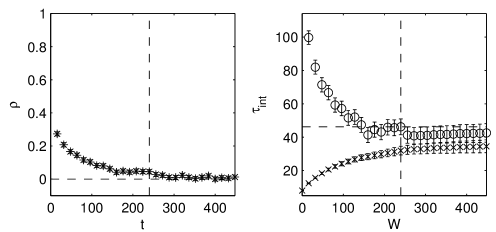
Figure 3: (Left) Auto-correlation function of the pseudo-scalar meson mass. The meson mass is obtained from a plateau average. (Right) Sum of the normalized auto-correlation function up to a window $W$. The cross indicates the truncated sum as in eq. 2. With the empty circle we denote the upper bound as defined in eq. 5. The vertical line denotes the window chosen with the three sigma criterion, while the horizontal marks the corresponding value of $\tau_{\mathrm{int}}^{u}$.

For this second part of the analysis we will use the mass of the quenched pseudo-scalar meson $c\bar{c}^{\prime}$ (consisting of two quarks with mass $m_{c}=m_{c^{\prime}}=m_{\text{charm}}$) obtained by averaging over a suitably chosen plateau. The upper bound formula eq. 5 requires a prescription on how to choose the window $W_{u}$. The criterion here used is that $\rho(W_{u})\simeq 3\delta\rho(W_{u})$. If the auto-correlation function falls off very quickly, then we choose the minimum $\tau_{\mathrm{int}}^{u}$ between the one evaluated at $W_{u}$ and the one evaluated at $W_{u}+\delta W$ (using eq. 5), where $\delta W$ is the MC distance between measurements. In Fig. 3 we compare two estimators of $\tau_{\mathrm{int}}$: our proposed upper bound and the sum in eq. 2 truncated at a window $W$ (without compensating for the tail at $t>W$). At small window size it is clearly visible that the upper bound overestimates the value of $\tau_{\mathrm{int}}$, but at $W\sim 100$ the estimator seems to settle on a plateau that extends to much larger values of the window, eventually overlapping with the “lower bound” estimates coming from below. This is a first indication of the fact that in situations where a tail is visible on the observable of interest (i.e. $m_{c}$) a knowledge coming from the slower sectors of the simulation (i.e. $\tau_{*}$) can effectively be used for a more reliable, possibly semi-automated, error analysis.

When we compare our method to the one in [3], where an optimal truncation window $W_{\text{opt}}$ is chosen by minimizing the sum of statistical and systematic error, we obtain, in this particular case, a window $W_{\text{opt}}=W_{u}$ and a value of $\tau_{\mathrm{int}}=30(2)$. Our method gives $\tau_{\mathrm{int}}^{u}=47(4)$, translating in an increase of $\approx 25\%$ on the estimated statistical error (see eq. 3). When specifically studying properties of the algorithm, we propose to use the two methods as upper/lower bound estimates of the true value of $\tau_{\mathrm{int}}$. In case one is interested in a reliable estimate of the error of physical observables however, we strongly suggest the use of $\tau_{\mathrm{int}}^{u}$. What we have shown so far is evidence that the upper bound gives a considerable, yet reasonable, increase in the error bars. In the next section we provide more evidence that the method still works reasonably well in presence of shorter MC histories.

4 Upper bound with lower statistics

As a complementary check of the validity of the arguments presented so far, it is interesting to study the upper bound formula in a case in which the length of the MC history is short (of the order of $10\times\tau_{*}$, for example). The reason for this is that, in the end, we want to apply this method of error analysis to simulations performed with dynamical fermions, where the computational costs can be very high. This makes a detailed study as the one presented here prohibitively expensive. Here our the total statistics is around $500\times\tau_{*}$, making it possible to perform a statistical study by splitting the whole history in bins of $3500$ MD units. On each of these shorter histories we have then calculated the auto-correlation function. To test the method we have assumed that $\tau_{*}$ is known (either from a previous study or from a model as proposed in [2]). In practice we have used the value of $\tau_{*}$ obtained from the auto-correlation function of $Q^{2}$ on the entire history.

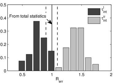
Figure 4: Comparison between standard definition of $\tau_{\mathrm{int}}^{l}$ and our improved estimate $\tau_{\mathrm{int}}^{u}$, normalized by the high statistics estimate, indicated by the vertical lines.

The comparison is shown in Fig. 4, in the form of two histograms in which we have binned the values

$$R_{\text{err}}=\sqrt{\left(\tau_{\mathrm{int}}^{\text{Bound}}/\tau_{\mathrm{int}}\right)}\;,$$ (7)

where $\tau_{\mathrm{int}}^{\text{Bound}}$ stands for either the upper bound $\tau_{\mathrm{int}}^{u}$ (computed with eq. 5) or the lower bound $\tau_{\mathrm{int}}^{l}$ (computed by truncating the sum at $W_{\text{opt}}$, as explained before) and $\tau_{\mathrm{int}}$ stands for the integrated auto-correlation time obtained from the whole history (no splitting). $R_{\text{err}}$ represents the relative deviation of the error extracted from limited statistics to the more realistic error, obtained from a more precise knowledge of the auto-correlation time. We observe that with the standard method, the error is always underestimated, up to a factor of two. These distributions teach the following lesson. The improved error estimate of eq. 5 is always safely close to the true error or somewhat above it. An error estimate using $\tau_{\mathrm{int}}^{u}$ is recommended. The histograms also remind us of an obvious fact: typically the error of the statistical error is not that small in QCD simulations.

5 Summary

In this study we have shown a method for safer error estimates in the limit of low statistics/long auto-correlation times. We first have applied the method to the error analysis of a quenched observable, illustrating also a method for extracting the contribution coming from the slowest known sectors of the simulation (i.e. smeared topological charge square).

We have then studied the method in the context of low statistics, showing that also in this regime the resulting estimates are not overly conservative and are therefore a safer way to determine the error. As discussed above, the proposed procedure for the improved error estimate can be automated. For this purpose, we have written a matlab routine that will be made publicly available soon.