Diffusive Counter Dispersion of Mass in Bubbly Media

Abstract

We consider a liquid bearing gas bubbles in a porous medium. When gas bubbles are immovably trapped in a porous matrix by surface-tension forces, the dominant mechanism of transfer of gas mass becomes the diffusion of gas molecules through the liquid. Essentially, the gas solution is in local thermodynamic equilibrium with vapor phase all over the system, i.e., the solute concentration equals the solubility. When temperature and/or pressure gradients are applied, diffusion fluxes appear and these fluxes are faithfully determined by the temperature and pressure fields, not by the local solute concentration, which is enslaved by the former. We derive the equations governing such systems, accounting for thermodiffusion and gravitational segregation effects which are shown not to be neglected for geological systems—marine sediments, terrestrial aquifers, etc. The results are applied for the treatment of non-high-pressure systems and real geological systems bearing methane or carbon dioxide, where we find a potential possibility of the formation of gaseous horizons deep below a porous medium surface. The reported effects are of particular importance for natural methane hydrate deposits and the problem of burial of industrial production of carbon dioxide in deep aquifers.

I Introduction

The diffusion of solute gases in liquids is a well-studied and relatively well-understood problem; see, e.g. Hirschfelder et al. (1954); Bird et al. (2007). In the classical formulation of the problem, the diffusion flux of guest atoms or molecules is expressed in terms of various thermodynamic “forces”—concentration, pressure, and temperature gradients. Usually, the liquid-gas interface does not influence the nature of the bulk diffusion and determines only the boundary conditions for the flux. There exists, however, a vast class of systems, called “bubbly liquids”, e.g. Yurkovetsky and Brady (1996), where the liquid-gas interface maintains the gas-solution saturation all over the liquid volume and serves as a source/sink for the diffusion flux of the solute molecules (i.e., the diffusion flux does not change the solute concentration with time, but redistributes the mass between gas bubbles). Thus the liquid-gas interface plays an important role in the bulk diffusion of solutes. On the macroscopic scale, the diffusive mass transport of solutes may be very unusual and surprising in these systems.

In the present study, we address bubbly liquids with immobile bubbles. These may be trapped by the surface forces in a porous matrix, therefore, for concreteness, we will consider liquids in porous media. Among numerous examples of such systems, which are of great practical importance, are the oil-bearing porous massifs, seabeds in organic carbon-rich marine sediments Archer (2007); Davie and Buffett (2001, 2003); Garg et al. (2008); Haacke et al. (2008), aquifers Donaldson et al. (1997, 1998), peat-bogs and swamps. For these systems, the presence of immobilized gas bubbles or liquid drops is well established experimentally. The respective solute gases include methane, carbon dioxide, oxygen, nitrogen, etc. Moreover, the problem of diffusion of the carbon dioxide in porous medium, filled with bubbly liquid (water) is directly related to the problem of burial of industrial release of $\mathrm{CO_{2}}$, e.g. Holloway (1997); Rochelle et al. (2009). In Fig. 1, we sketch a typical system, where the diffusion of a solute gas takes place in a bubbly liquid in a porous matrix.

We will study diffusion transport on large space and time scales. Namely, we will be interested in the space scale much larger than the characteristic size of a gas bubble and in the time scale much larger than the characteristic relaxation time for gas dissolution in liquid; hence we assume that all over the volume, the solute gas is saturated in the solution. Indeed, for marine sediments the solution relaxation times measured by hours are small compared to the global evolution time scales, which can be as large as millions of years. To estimate the pore size $l$ needed to trap a bubble of the comparable size we notice that the surface-tension forces, equal to $\sigma l$ ($\sigma$ is the surface tension), should overwhelm the buoyancy force $\rho_{\mathrm{liq}}gl^{3}$ ($\rho_{\mathrm{liq}}$ is the density of a liquid; $g$ is the gravity). This yields the estimate, $l<\sqrt{\sigma/\rho_{\mathrm{liq}}g}$, implying the maximal pore size $l<2.7\,{\rm mm}$ for water, which suggests trapping even for sands. We consider the immobilization of pore-size bubbles, because a big moving bubble is unstable to splitting Lyubimov et al. (2009); it either stops or experiences splitting into smaller bubbles until their size becomes comparable to the pore size. We assume that our space scale is much larger than $l$. It is not straightforward to estimate the relaxation time for the gas dissolution; therefore, we just assume that the condition of the gas saturation in liquid is always fulfilled.

Another important feature of bubbly liquids in porous media (relevant for many geological systems) is the presence of a temperature gradient (usually due to the geothermal gradient) and a pressure gradient (due to the hydrostatic pressure). On the microscopic level, the temperature gradient causes the thermodiffusion (the so-called “Soret effect” Sorét (1879); Jones and Furry (1946); Hirschfelder et al. (1954); Bird et al. (2007)), while the pressure gradient manifests the presence of the gravitational forces. Due to different mobilities and masses of the solute and solvent molecules these may cause an additional mass flux. Although the importance of thermodiffusion for soil gas exchange has been reported in Ref. Richter (1972), only the diffusion flux due to the concentration gradient (Fickian diffusion) has been investigated so far Davie and Buffett (2001, 2003); Garg et al. (2008); Haacke et al. (2008).

In the present study, we consider the diffusive transport of a solute gas in liquid in a porous medium without any significant through-flow in the system; that is, we consider only molecular and not hydrodynamic diffusion Donaldson et al. (1997, 1998); Saffman (1959); Sahimi (1993). We show that for large space and time scales, which assume the saturation condition for the solute gas, and under temperature and pressure gradients a novel and interesting phenomenon may be observed—the diffusive accumulation of gas in certain regions, caused by the non-Fickian transport of solutes.

The paper is organized as follows. In Sec. II the diffusion flux of a solute gas in bubbly liquid is considered in the presence of pressure and temperature gradients; the evolution equation for the gas concentration is obtained. In Sec. III we demonstrate the existence of a novel phenomenon—the diffusive accumulation of solute gas in certain regions. We analyze this effect for real geological systems—the methane or carbon dioxide bearing massifs in the presence of the geothermal gradient. Finally, in Sec. IV, we summarize our findings. Some technical details are given in the Appendixes.

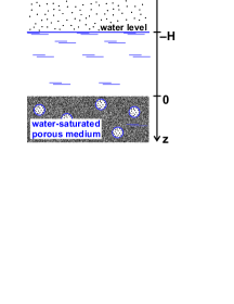
Figure 1: Typical system of bubbly liquid filling the porous medium. The pressure, temperature, and parameters of the porous matrix may vary vertically, but are constant horizontally. The figure, with water above the bubble-rich sediments, sketches numerous geological systems.

II Diffusion transport in bubbly liquid with gradients of thermodynamic properties

The diffusion current of guest particles in a host material in the presence of concentration and temperature gradients and an external potential generally has three components, each being the response to their respective driving force: The Fickian flux, due to the concentration gradient, the thermodiffusion flux, due to the temperature gradient, and the flux due to the mobility of particles subjected to an external force. When there are no external forces except gravity, which also creates the pressure gradient, the diffusion flux of a dilute solution reads Bird et al. (2007)

$$\vec{J}=-DX\left[\frac{\nabla X}{X}+\alpha_{T}\frac{\nabla T}{T}-\frac{\tilde{M}\vec{g}}{RT}\right],$$ (1)

where $X$ is the molar fraction (concentration) of the solute in the solution, $D$ is the molecular diffusion coefficient of the solute molecules in the solvent, $\alpha_{T}$ is the thermodiffusion constant ($\alpha_{T}/T$ is the Soret coefficient), and $R=8.31{\rm J\,K^{-1}mol^{-1}}$ is the universal gas constant. $\tilde{M}=M^{\mathrm{g}}-N_{1}M^{\mathrm{host}}$, where $M^{\mathrm{g}}$ and $M^{\mathrm{host}}$ are the molar masses of solute and solvent molecules, and $N_{1}$ is the number of solvent molecules in the volume occupied by one solute molecule in the solution. For specific gases we derive $N_{1}$ from experimental data in Appendix A.

When the liquid is saturated with gas bubbles and the bubbles are in local thermodynamic equilibrium with the solution, the concentration of the solute in the solvent equals solubility, $X=X^{(0)}$, everywhere in the liquid. The thermodynamic equilibrium implies the equality of the chemical potentials of the gas dissolved in the liquid ($\mu_{\mathrm{liq}}^{\mathrm{g}}$) and that of the vapor phase ($\mu_{\mathrm{vap}}^{\mathrm{g}}$), that is, $\mu_{\mathrm{liq}}^{\mathrm{g}}=\mu_{\mathrm{vap}}^{\mathrm{g}}$. According to the thermodynamic laws, the chemical potential of the vapor phase depends exclusively on temperature $T$ and pressure $P$, $\mu_{\mathrm{vap}}^{\mathrm{g}}=\mu_{\mathrm{vap}}^{\mathrm{g}}(T,P)$. Hence the solute concentration $X$ is not a free variable, but a function of the local temperature and pressure, $X(\vec{r})=X^{(0)}\left(T(\vec{r}),P(\vec{r})\right)$; the same holds true for the solute flux $\vec{J}(\vec{r})$. In Appendix B of this paper we provide the calculation of high-pressure aqueous solubility of gases based on a scaled particle theory Pierotti (1976) amended with implementation of van der Waals’ equation of state for the vapor phase.

In the present study we consider the problem of diffusion transport in a bubbly liquid in the context of real geological systems, where pressure varies from one to a few hundred atmospheres (this refers to a few kilometers deep water column, see Fig. 1). To illustrate the approach, we will discuss first a more simple case of moderate pressures $P<100\,{\rm atm}$, which allows an explicit analytical treatment. The results for the general case, obtained numerically, will be also shown.

According to Eq. (20) in Appendix B, for moderate pressures and far from the solvent boiling temperature the solubility depends on $T$ and $P$ as follows

$$X^{(0)}(T,P)\simeq X^{(0)}(T_{0},P_{0})\frac{T_{0}}{T}\frac{P}{P_{0}}\exp\left[q\left(\frac{1}{T}-\frac{1}{T_{0}}\right)\right]\,,$$

where $T_{0}$ and $P_{0}$ are reference values, the choice of which is guided merely by the convenience reason, and $X^{(0)}(T_{0},P_{0})$ is the solubility at the reference temperature and pressure; the parameter $q\equiv-G_{i}/k_{\mathrm{B}}$ is given in Tab. 1. Pressure is moderate in a sense that one can neglect van der Waals’ effects and the influence of pressure on the Gibbs free energy of the cavity formation for the guest molecule in the solvent. The latter is represented by the term $(-BP/T)$ in the exponential of Eq. (20), where constant $B\approx 10^{-6}\,{\rm K/Pa}$ (see Tab. 1), and becomes significant only for pressures as high as several hundreds atmospheres. The limiting formula is free of the molar fraction $Y$ [Eq. (21)] of the solvent molecules in gas bubbles because it is assumed to be zero. This assumption is valid several tens of Kelvins below the water boiling temperature, while the systems where liquids are at near-boiling conditions, say geysers, are beyond the scope of the present study.

Using $\nabla X^{(0)}=X^{(0)}[P^{-1}\nabla P-(1+q/T)T^{-1}\nabla T]$, one obtains for the total flux:

$$\vec{J}\simeq-DX^{(0)}\left[\frac{\nabla P}{P}-\left(1-\alpha_{T}+\frac{q}{T}\right)\frac{\nabla T}{T}-\frac{\tilde{M}\vec{g}}{RT}\right].$$ (2)

Note that the flux does not depend on the solute concentration or its gradient as independent fields.

Generally, the flux (2) possesses a nonzero divergency $\nabla\cdot\vec{J}$, which implies the existence of sources and sinks for the solute mass. Obviously, the gas bubbles serve as the mass reservoir, which provides the respective sources and sinks. Hence the mass balance reads

$$\frac{\partial X_{\mathrm{b}}}{\partial t}+\nabla\cdot\vec{J}=0\,,$$ (3)

where $X_{\mathrm{b}}$ is the molar fraction of bubbles in the bubbly fluid, that is, in the system comprised by bubbles and liquid. For the space scales addressed here we do not need to consider the microscopic processes of the bubbles growth and clustering as in Dominguez et al. (2000), and the single characteristic, $X_{\mathrm{b}}(\vec{r})$, suffices in our case.

Hence for moderate pressures we obtain the following equation for the evolution of a nondissolved gas phase:

$$\frac{\partial X_{\mathrm{b}}}{\partial t}\simeq\nabla\cdot\left(DX^{(0)}\left[\frac{\nabla P}{P}-\left(1-\alpha_{T}+\frac{q}{T}\right)\frac{\nabla T}{T}-\frac{\tilde{M}\vec{g}}{RT}\right]\right).$$ (4)

Eqs. (3) and (4) are written for the case when the bubbles occupy a small fraction of the fluid volume, which is typical for most geological systems, e.g. Davie and Buffett (2001, 2003). Moreover, the corrections needed to account for the finite fraction of the bubble volume are always quantitative and never qualitative. Indeed, the direction of the solute flux is merely determined by the factor in the square brackets in the right-hand side of Eq. (4), which does not depend on the bubble volume.

III The diffusive accumulation and non-Fickian flux of solutes

In what follows we consider the one-dimensional diffusion of solutes in bubbly liquids in the presence of temperature and density gradients, using for the latter quantities some typical geological values. The model of one-dimensional diffusion is motivated by the fact that real geological systems are much more uniform along two directions (say horizontal) than along the third direction (say vertical). Then we have a laterally uniform system with vertical gradients of its thermodynamic properties. For the sake of definiteness we analyze the case of seabed sediments, Fig. 1, where the depth below the seafloor is measured by the $z$ coordinate. Then we have $z$-dependent hydrostatic pressure and $z$-dependent temperature due to the geothermal temperature gradient:

$$P(z)=P_{0}+\rho_{\mathrm{liq}}g(z+H),\qquad T(z)=T_{\mathrm{sf}}+Gz.$$

Here $P_{0}$ is the atmospheric pressure, $H$ is the height of the pure-water layer above the bubble-bearing porous medium, $T_{\mathrm{sf}}$ is the temperature of the seafloor and $G$ is the geothermal gradient. Nonlinearity of the temperature profile Goldobin (2011) is neglected in our study because it is system specific and not a principal ingredient for the phenomenon we consider. The assumption of a linear temperature profile is typical for studies on physical processes in marine sediments Davie and Buffett (2001, 2003).

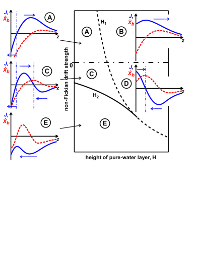
Figure 2: (Color online) Diagram of diffusive regimes on the plane $\beta$–$H$ ($\beta$ quantifies the non-Fickian drift strength) for moderate pressures. The critical heights $H_{1}$ and $H_{2}$ are given by Eqs. (6) and (7), respectively. In the plug-in plots the dependence of the solute flux $J$ (blue solid lines) and of the bubble growth rate $\dot{X}_{b}$ (red dashed lines) on the depth $z$ below the seafloor is shown.

(a)
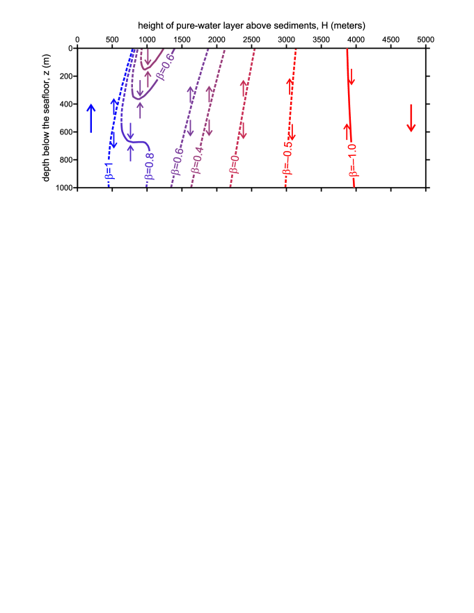
(b)

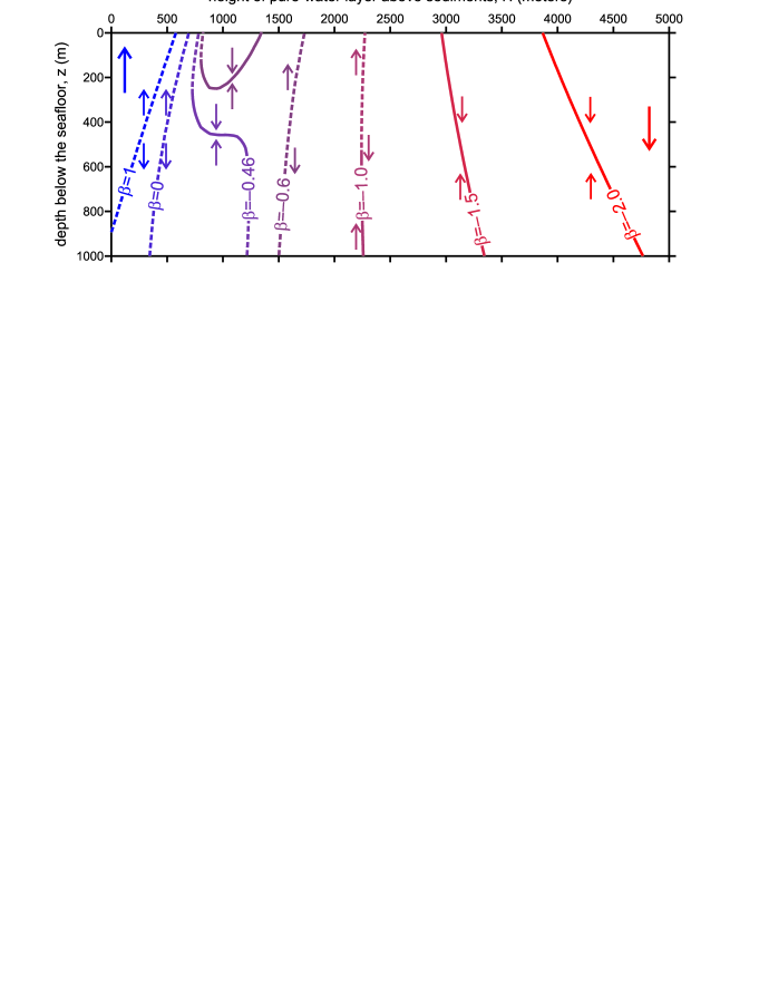
Figure 3: (Color online) Direction of the mass flux and the position of the flux inversion point as the function of the height of pure-water column above the sediments. Different curves correspond to different values of the non-Fickian parameter $\beta$ for methane. Calculations have been performed for the seafloor temperature $T_{\mathrm{sf}}=277{\rm K}$ and geothermal gradient $G=40{\rm K/km}$ (a) and $G=60{\rm K/km}$ (b) for the general case, without the approximation of moderate pressures. The flux inversion points with negative divergency (accumulating the solute gas) are plotted with the solid curves, the points with positive divergency (“repelling” the solute gas) are shown with the dashed curves.

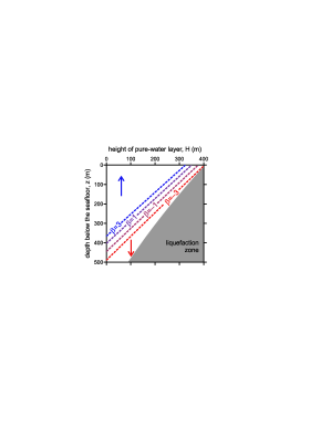
Figure 4: (Color online) Direction of the mass flux and the position of the flux inversion point for carbon dioxide. Calculations have been performed for the seafloor temperature $T_{\mathrm{sf}}=277\,{\rm K}$ and geothermal gradient $G=40\,{\rm K/km}$ for the general case, that is, without the the approximation of moderate pressures. For details see the caption for Fig. 3.

Using the above expressions for the hydrostatic pressure and geothermal gradient, we obtain for the diffusion flux (2) for moderate pressures:

$$J\simeq DX^{(0)}\left[-\frac{1}{z+H+P_{0}/\rho_{\mathrm{liq}}g}\right.\qquad\qquad$$

$$\left.+\left(1+\beta+\frac{q}{T_{\mathrm{sf}}+Gz}\right)\frac{1}{z+T_{\mathrm{sf}}/G}\right],$$ (5)

where

$$\beta\equiv-\alpha_{T}+\frac{\tilde{M}g}{RG}.$$

Eq. (5) with $\beta=0$ corresponds to the Fickian diffusion, $\vec{J}=-D\nabla{X}$, while the coefficient $\beta$ quantifies the strength of the non-Fickian contribution to diffusion flux. Let us consider the consequences of the above model for the typical geological systems, like marine sediments. Fig. 2 illustrates the variety of possible diffusive regimes. For the gases with positive $\beta$, the gas leaves the sediments. In shallow seas the gas diffuses upwards, to the sea, in the thin upper layer of sediments and downwards below this layer [regime (A) in Fig. 2]. When the sea depth $H$ exceeds a certain value $H_{1}$, the upper layer disappears and the gas diffuses downwards all over the seabed [regime (B)]; for moderate pressures the threshold depth reads,

$$H_{1}=\frac{T_{\mathrm{sf}}}{G\left(\displaystyle 1+\beta+q/T_{\mathrm{sf}}\right)}-\frac{P_{0}}{\rho_{\mathrm{liq}}g}.$$ (6)

For gases with negative $\beta$, the direction of the flux very deep below the seafloor turns upwards. In deep seas, $H>H_{1}$ [regime (D)], the solute accumulation zone appears: The solute gas from the upper and deep layers of sediments diffuses to this zone. For shallow seas, $H<H_{1}$ [regime (C)], the solute gas accumulation zone loses its contact with the seafloor. In this case the solute gas from the region just beneath the seafloor migrates upwards, to the sea.

Thus we reveal a novel and surprising phenomenon—the formation of a gas accumulation zone: Instead of the tendency of the gas to spread uniformly over the system, as expected for the common diffusion, the gas concentrates in narrow zones, due to the non-Fickian diffusion against the direction dictated by the concentration gradient.

Finally, if the positive thermodiffusion is strong enough, one observes the regime (E), where no gas-retracting zone exists and all the solute migrates upwards, to the sea. Nevertheless, the inhomogeneity of the diffusion flux results in the bubble growth zone. For moderate pressures, the depth $H$ of the water body beneath which this diffusion regime occurs is bounded from above by

$$H_{2}=\frac{T_{\mathrm{sf}}}{G}-\frac{P_{0}}{\rho_{\mathrm{liq}}g}-\frac{q}{G\left(1+\sqrt{-\beta}\right)^{2}}$$ (7)

$$\mbox{ for }\beta\in\left[-\frac{1}{4}\left(\sqrt{1+\frac{4q}{T_{\mathrm{sf}}}}-1\right)^{2},\right.$$

$$\qquad\qquad\qquad\left.-\left(\sqrt{\frac{q}{T_{\mathrm{sf}}-P_{0}G/\rho_{\mathrm{liq}}g}}-1\right)^{2}\right].$$

For high pressure, the solubility and diffusion flux are more gas-specific and each particular case requires a separate analysis. In Figs. 3 and 4, the results for methane and carbon dioxide are shown for the general case, where Eqs. (1), (20), and (21) have been used without the simplifying approximations adopted for the moderate pressures. The range of parameters used in Figs. 3 and 4 is chosen to be relevant for practical applications: The range of pressures for methane corresponds to the possible location of the gas-hydrate deposits (methane is one of the components of the hydrate), while the pressures for carbon dioxide may be essential for the process of burial of industrial $\mathrm{CO_{2}}$ in deep aquifers.

For methane (Fig. 3), we consider the upper $1-{\rm km}$ layer of sediments for sea depths ranging from $0\,{\rm km}$ to $5\,{\rm km}$ with the seafloor temperature $T_{\mathrm{sf}}=277\,{\rm K}$ (which corresponds to maximal water density at atmospheric pressure). For a small geothermal gradient, $G=20\,{\rm K/km}$, methane diffuses upwards, to the sea, for any value of the non-Fickian parameter $\beta$ and any sea depth $H$. For a larger $G$, the transport significantly depends on $\beta$ and $H$ (Fig. 3). For the typical value of $G=\,40{\rm K/km}$ Davie and Buffett (2001, 2003) methane diffuses upwards in shallow seas and downwards for deep ones; the sea depth $H$ for which the flux at $z=0$ reverses increases as $\beta$ decreases. Remarkably, for the range of the non-Fickian parameter $0.3\lesssim\beta\lesssim 0.9$, the gas accumulation zone (which blocks the release of methane into the sea) is located in the seabed at the depth ranging from $0.7\,{\rm km}$ to $1.6\,{\rm km}$ (solid lines in Fig. 3a). For $\beta\lesssim-1$, this zone appears in sediments under deep water bodies, $H\gtrsim 3.9\,{\rm km}$. In Fig. 3b, where $G=60\,{\rm K/km}$, one can see how the diffusion regimes are affected by further increase of the geothermal gradient. We wish to stress, that the reported phenomenon originates exclusively due to the non-Fickian diffusion. The oversimplified models based on the Fickian law with $\beta=0$, e.g. Davie and Buffett (2001, 2003), cannot describe the novel effect of the formation of gas accumulation zone.

The main difficulty of the practical application of our theory is the lack of precise data for the thermodiffusion constant, that is, the lack of a trustworthy value for the coefficient $\beta$. For instance, the authors are not aware of any experimental data on the thermodiffusion of methane in water. Theoretical studies, e.g. Semenov (2010), do provide the first-principle expressions for computing the thermodiffusion constant. These, however, require the knowledge of the intermolecular potentials and structural properties of the solvent. Hence, to obtain a reliable estimate for the non-Fickian parameter, extensive numerical simulations by means of Molecular Dynamics or Monte Carlo are needed, which is beyond the scope of the present study. Presently, however, we can prospect the value of $\alpha_{T}$ from a simplified model of a large Brownian chemically-inert particle in non-isothermal liquids. With this model, $\alpha_{T}$ is controlled merely by the volume per one guest molecule in the solution and the guest molecule mass; employing Buckingham’s $\pi$-theorem of dimensional analysis Buckingham (1914) one can make an interpolation of the data for dilute aqueous solutions of paraffin alcohols: $\alpha_{T}\approx 1.5$ for methanol Tichacek et al. (1956), $\alpha_{T}\approx 3.0$ for ethanol Kita et al. (2004), and $\alpha_{T}\approx 4.5$ for isopropanol Poty et al. (1974). This interpolation yields $\alpha_{T}\approx 1.8$ for methane. Thus, $\beta^{\mathrm{CH_{4}}}\approx-2.5$ for aqueous solutions in the presence of geothermal gradient $G=40\,{\rm K/km}$, and $\beta^{\mathrm{CH_{4}}}\approx-2.3$ for $G=60\,{\rm K/km}$.

For the case of carbon dioxide the non-Fickian drift affects the solute flux much more weakly than for methane (Fig. 4). Under shallow water bodies, ${\rm CO_{2}}$ diffuses upwards in upper layers of sediments, and downwards for deep layers.

IV Conclusion

We have developed the theoretical description of the process of diffusive migration of a dissolved gas in bubbly liquids, where bubbles are immovably trapped by a porous matrix, as in a seabed or terrestrial aquifers. The effect of temperature inhomogeneity across the system and the gravity force are accounted for. The theory is employed for treatment of typical geological systems with the hydrostatic pressure distribution and the geothermal gradient.

For non-high pressure the diffusion flux and bubble mass evolution are governed by Eqs. (2) and (4), respectively; Fig. 2 presents the diagram of diffusive regimes derived for these equations. For high pressure the system is comprehensively described by Eqs. (1), (20), and (21) with parameters provided in Tab. 1 for four typical gases: nitrogen, oxygen, carbon dioxide, and methane. The high-pressure solubility (20) has been derived from the standard scaled particle theory Pierotti (1976) with adoption of van der Waals equation of state.

The “non-Fickian” corrections—thermodiffusion and gravitational segregation—appear to play an essential role in migration of methane in the seabed, even being able to create the gaseous methane accumulation zone in sediments (Fig. 3). For carbon dioxide the non-Fickian effects are not as significant: they do not cause the qualitative change of behavior but can only shift the boundary of the $\mathrm{CO_{2}}$-capture zone by not more than $75\,{\rm m}$, which is $15\%$ of the characteristic depth (Fig. 4). Unfortunately, the precise values of the thermodiffusion constant of aqueous solutions of methane or carbon dioxide are not found in the literature, and one can only estimate their values as we do in this paper. The practical significance of the thermodiffusion effect, which has become apparent for the evolution of geological systems, necessitates the experimental determination of the thermodiffusion constant for aqueous solutions of methane and carbon dioxide.

Appendix A Calculation of $N_{1}$ and $\tilde{M}$ from experimental data

The ratio of the volume occupied by one mole of solute molecules in the solvent, $v_{\mathrm{liq}}^{\mathrm{g}}$, and the molar volume of this solvent, $v_{\mathrm{liq}}$, [which is $N_{1}=(v_{\mathrm{liq}}^{\mathrm{g}}/v_{\mathrm{liq}})$ in Sec. II] can be precisely derived for $\mathrm{CO_{2}}$–$\mathrm{H_{2}O}$ and $\mathrm{CH_{4}}$–$\mathrm{H_{2}O}$ systems from the dependence of the solution density on its concentration, which is available in the literature Hnedkovsky et al. (1996); Garcia (2001); Duan et al. (2008). The molar volume of solution is $v_{\mathrm{sol}}=v_{\mathrm{liq}}(1-X)+v_{\mathrm{liq}}^{\mathrm{g}}X$, and the density is

$$\rho_{\mathrm{sol}}=\frac{M^{\mathrm{host}}(1-X)+M^{\mathrm{g}}X}{v_{\mathrm{sol}}}$$

$$\quad=\rho_{\mathrm{sol}}(X=0)\left[1+\left(\frac{M^{\mathrm{g}}}{M^{\mathrm{host}}}-\frac{v_{\mathrm{liq}}^{\mathrm{g}}}{v_{\mathrm{liq}}}\right)X+O(X^{2})\right],$$

where $M^{\mathrm{host}}$ and $M^{\mathrm{g}}$ are the molar masses of the solvent and solute molecules, respectively; $\rho_{\mathrm{sol}}(X=0)=\rho_{\mathrm{liq}}$ is the density of a pure liquid (solvent). Hence,

$$\frac{v_{\mathrm{liq}}^{\mathrm{g}}}{v_{\mathrm{liq}}}=\frac{M^{\mathrm{g}}}{M^{\mathrm{host}}}-\frac{1}{\rho_{\mathrm{liq}}}\frac{\partial\rho_{\mathrm{sol}}}{\partial X},\quad\tilde{M}=\frac{M^{\mathrm{host}}}{\rho_{\mathrm{liq}}}\frac{\partial\rho_{\mathrm{sol}}}{\partial X}.$$ (8)

The results of the implementation of the latter relation to the experimental data from Hnedkovsky et al. (1996); Garcia (2001) are summarized in the three last columns of Table 1.

Appendix B Aqueous solubility of certain gases

Here we wish to present some detail of our calculations, outlined in previous sections. To evaluate the solubility at high pressure we make a straightforward generalization of the standard scaled particle theory. Namely, instead of the ideal-gas equation of state we use the van der Waals equation for the vapor phase of the dissolved gas. We find the chemical potential of the solute and calculate solubility for the gases, most important for applications—oxygen, nitrogen, carbon dioxide, and methane.

B.1 Chemical potential in the vapor phase

To introduce notations and recall basic relations we start from an ideal gas. The Helmholtz free energy, $F(T,V,N)$, the Gibbs free energy, $G(T,P,N)=F+PV=F-V(\partial F/\partial V)$, and the chemical potential, $\mu_{\mathrm{vap}}^{\mathrm{g}}(T,P)=\partial G(T,P,N)/\partial N$, read for an ideal gas,

$$F = -Nk_{\mathrm{B}}T\ln\frac{eV}{N}+Nk_{\mathrm{B}}T\ln\frac{\Lambda^{3}}{Z(T)}\,,$$ (9)

$$G = Nk_{\mathrm{B}}T\ln\frac{P}{k_{\mathrm{B}}T}+Nk_{\mathrm{B}}T\ln\frac{\Lambda^{3}}{Z(T)}\,,$$ (10)

$$\mu_{\mathrm{vap}}^{\mathrm{g}} = k_{\mathrm{B}}T\ln\left[\frac{P}{k_{\mathrm{B}}T}\,\frac{\Lambda^{3}}{Z(T)}\right]\,,$$ (11)

where $N$ is the number of molecules, $V$ is the volume, $P$ is pressure, $k_{\mathrm{B}}$ is the Boltzmann constant, $\Lambda=\sqrt{2\pi\hbar^{2}/mk_{\mathrm{B}}T}$ is the thermal de Broglie wavelength of a gas molecule of mass $m$, $\hbar$ is the Planck constant divided by $2\pi$ and $Z(T)$ is the partition function of the internal degrees of freedom of the molecule. It depends on the molecular structure and temperature.

Now, we address the chemical potential of real gases, taking into account the finite volume fraction of the gas molecules and their attractive interactions. The simplest way to do this is to use the van der Waals model. We assume that the heat capacity $c_{V}$ does not depend on temperature. This is justified for the range of temperatures of interest for many gases, including methane. Then the Helmholtz and Gibbs free energies read, e.g. Landau and Lifshitz (1996),

$$F(T,V,N) = F_{\mathrm{id.}}-Nk_{\mathrm{B}}T\ln\left(1-nb\right)-Nna,$$ (12)

$$G(T,P,N) = G_{\mathrm{id.}}-Nk_{\mathrm{B}}T\ln\left(1-nb\right)$$ (13)

$$\qquad{}-2Nna+Nk_{\mathrm{B}}T\frac{nb}{1-nb}\,.$$

Here $F_{\mathrm{id.}}$ and $G_{\mathrm{id.}}$ are the respective ideal parts and $a$ and $b$ are the van der Waals constants (see Tab. 1 for the specific values). Note that above the critical point of a gas ($T_{c}=-82.7\,^{\circ}\mathrm{C}$ for methane), $n=n(P)$ is a univocal function of pressure, which may be obtained from the van der Waals equation of state:

$$P=\frac{nk_{\mathrm{B}}T}{1-nb}-an^{2}\,.$$ (14)

Finally, the chemical potential of the van der Waals gas reads,

$$\mu_{\mathrm{vap}}^{\mathrm{g}}(T,P)=k_{\mathrm{B}}T\left[\ln\left(\frac{n\Lambda^{3}}{Z(T)}\right)-\ln(1-bn)\right.\quad$$

$$\left.{}-\frac{2an}{k_{\mathrm{B}}T}+\frac{nb}{1-nb}\right].$$ (15)

This result can be found in Hirschfelder et al. (1954).

Table 1: Parameters of gases and their aqueous solutions. Values of $\sigma$, $B$, and $G_{i}$ are derived from the theoretical fitting of the experimental data presented in Fig. 5. Parameters in the three last columns are derived from experimental data Hnedkovsky et al. (1996); Garcia (2001) with Eq. (8).

	$\displaystyle a,\ \displaystyle{\rm\frac{m^{6}Pa}{mol^{2}}}$	$\displaystyle b,\ \displaystyle 10^{-5}{\rm\frac{m^{3}}{mol}}$	$\sigma$, ${\rm\AA}$	$A(y)$	$\displaystyle B,\ \displaystyle 10^{-6}{\rm\frac{K}{Pa}}$	$\displaystyle\frac{G_{i}}{k_{\mathrm{B}}}$, ${\rm K}$	$\displaystyle\frac{1}{\rho_{0}}\frac{\partial\rho_{\mathrm{sol}}}{\partial X}$	$N_{1}\equiv\displaystyle\frac{v_{\mathrm{liq}}^{\mathrm{g}}}{v_{\mathrm{liq}}}$	$\displaystyle\tilde{M},\ \displaystyle{\rm\frac{g}{mol}}$
$\mathrm{O_{2}}$	$0.1378$	$3.183$	$3.03$	$6.38$	$1.056$	$-873$	—	—	—
$\mathrm{N_{2}}$	$0.1408$	$3.913$	$3.15$	$6.77$	$1.182$	$-781$	—	—	—
$\mathrm{CO_{2}}$	$0.3640$	$4.267$	$3.02$	$6.36$	$1.050$	$-1850$	$0.54$	$1.91$	$9.7$
$\mathrm{CH_{4}}$	$0.2283$	$4.278$	$3.27$	$7.18$	$1.321$	$-1138$	$-1.35$	$2.24$	$-24.3$
$\mathrm{H_{2}O}$	—	—	$2.77$	—	—	—	—	—	—

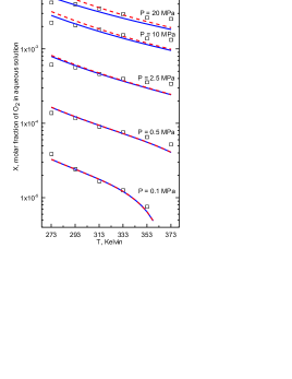
(a)       (b)

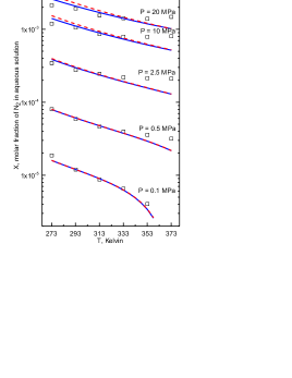
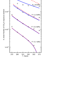
(c)       (d)

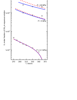
Figure 5: (Color online) Solubility of $\mathrm{O_{2}}$ (a), $\mathrm{N_{2}}$ (b), $\mathrm{CO_{2}}$ (c), and $\mathrm{CH_{4}}$ (d) in water at specified pressure. Squares represent experimental data (Baranenko et al. (1990a, b) for nitrogen, oxygen, and carbon dioxide and Yamamoto et al. (1976); Duan and Mao (2006) for methane); red dashed lines: results of the scaled particle theory for vapor phase assumed to be an ideal gas, Eq. (19); blue solid lines: the scaled particle theory with van der Waals’ equation of state for the vapor phase, Eq. (20).

B.2 Solubility of gas: Scaled particle theory

To evaluate the solubility of a gas in a solvent (water) we employ scaled particle theory (see e.g. the review Pierotti (1976) for detail). When the concentration of the dissolved gas reaches solubility, the system is in thermodynamic equilibrium, so that the chemical potential of the gas in the vapor phase $\mu_{\mathrm{vap}}^{\mathrm{g}}$ is equal to this in the solution $\mu_{\mathrm{liq}}^{\mathrm{g}}$. According to the scaled particle theory Pierotti (1976),

$$\mu_{\mathrm{liq}}^{\mathrm{g}}=G_{c}+G_{i}+k_{\mathrm{B}}T\ln(\Lambda^{3}/Z)+k_{\mathrm{B}}T\ln(XN_{\mathrm{A}}/v_{\mathrm{liq}}),$$ (16)

where $\Lambda$ and $Z$ are the de Broglie wavelength and the partition functions per molecule for the internal degrees of freedom for the solute, $X$ is the molar fraction of the gas, $G_{c}$ is the work of creation of a cavity for a guest molecule in the solvent, $G_{i}$ is the interaction energy between a solute molecule and the surrounding solvent molecules, $N_{\mathrm{A}}$ is the Avogadro number, and $v_{\mathrm{liq}}$ is the molar volume of the solvent particles (e.g. $v_{\mathrm{H}_{2}\mathrm{O}}=17.95\,{\rm cm^{3}/mol}$ at atmospheric pressure and $T=300\,{\rm K}$). The cavity formation work reads Pierotti (1976)

$$\frac{G_{c}}{k_{\mathrm{B}}T}=-\ln(1-y)+\frac{3y}{1-y}\frac{\sigma_{\mathrm{g}}}{\sigma_{\mathrm{liq}}}$$

$$\qquad{}+\left[\frac{3y}{1-y}+\frac{9}{2}\left(\frac{y}{1-y}\right)^{2}\right]\left(\frac{\sigma_{\mathrm{g}}}{\sigma_{\mathrm{liq}}}\right)^{2}$$

$$\qquad{}+\frac{yP}{n_{\mathrm{liq}}k_{\mathrm{B}}T}\left(\frac{\sigma_{\mathrm{g}}}{\sigma_{\mathrm{liq}}}\right)^{3}\equiv A(y)+B(y)\frac{P}{T},$$ (17)

where $\sigma_{\mathrm{liq}}$ and $\sigma_{\mathrm{g}}$ are respectively the effective diameter of the solvent (liquid) and solute (gas) molecules, $n_{\mathrm{liq}}$ is the number density of solvent, and $y=(\pi/6)n_{\mathrm{liq}}\sigma_{\mathrm{liq}}^{3}$ (e.g., $y_{\mathrm{H_{2}O}}=0.371$ at $T=300\,{\rm K}$ Pierotti (1976)). There exist numerous models for the interaction energy $G_{i}$ (e.g. Pierotti (1976); Hildebrand and Scott (1964)); for the present study it is enough, however, to mention that it is almost independent of pressure and temperature.

For the vapor phase, the chemical potential is given either by Eq. (11) for an ideal gas or by Eq. (15) with (14) for $n=n(P)$.

$$\mu_{\mathrm{vap}}^{\mathrm{g}}=k_{\mathrm{B}}T\ln(\Lambda^{3}/Z)+k_{\mathrm{B}}T\ln(f/k_{\mathrm{B}}T),$$ (18)

where $f$ is the fugacity of the gas molecules in the vapor phase. It is equal to the pressure for a one-component gas, and to the partial pressure for a gas mixture. In the case of interest, $f=P(1-Y)$, where $Y$ is the molar fraction of solvent vapor in the gaseous phase; it is determined by Eq. (21) below. Equating Eqs. (16) and (18) for the chemical potential, one finds the equilibrium molar fraction of the dissolved gas, that is the solubility, $X^{(0)}$. For an ideal gas one obtains, using Eq. (18) together with the ideal gas equation of state

$$X^{(0)}=\frac{(1-Y)P\,v_{\mathrm{liq}}}{RT}\exp\left[-\frac{G_{c}+G_{i}}{k_{\mathrm{B}}T}\right]$$

$$=\frac{(1-Y)P\,v_{\mathrm{liq}}}{RT}\exp\left[-A(y)-B\frac{P}{T}-\frac{G_{i}}{k_{\mathrm{B}}T}\right].$$ (19)

For a van der Waals gas, the real gas equation of state, Eq. (14), is to be employed. This yields

$$X^{(0)}=\frac{(1-Y)n\,v_{\mathrm{liq}}}{(1-nb)N_{\mathrm{A}}}\exp\left[-\frac{G_{c}+G_{i}}{k_{\mathrm{B}}T}-\frac{2an}{k_{\mathrm{B}}T}+\frac{1}{1-nb}\right]$$

$$=\frac{(1-Y)n\,v_{\mathrm{liq}}}{(1-nb)N_{\mathrm{A}}}\exp\left[-A(y)-B\frac{P}{T}-\frac{G_{i}}{k_{\mathrm{B}}T}\right.\quad$$

$$\left.{}-\frac{2an}{k_{\mathrm{B}}T}+\frac{1}{1-nb}\right].\qquad$$ (20)

When liquid with a dissolved gas is in equilibrium with its vapor phase, the vapor, including the vapor in bubbles, contains both components. Let us evaluate the solvent molar fraction $Y$ in the vapor phase. The enthalpy variation $dH=c_{P}dT+VdP=T\,dS+VdP$. Hence, $H=H_{0}+\int_{T_{0}}^{T}c_{P}(T_{1})\,dT_{1}+\int_{P_{0}}^{P}V(T,P)\,dP$, $S=S_{0}+\int_{T_{0}}^{T}c_{P}(T_{1})T_{1}^{-1}dT_{1}$, and Gibbs free energy $G=H-TS=H_{0}+\int_{T_{0}}^{T}c_{P}(T_{1})\,dT_{1}+\int_{P_{0}}^{P}V(T,P)\,dP-T\,S_{0}-T\int_{T_{0}}^{T}c_{P}(T_{1})T_{1}^{-1}dT_{1}$.

For liquid water, $c_{P}(T)$ is nearly constant and

$$G_{\mathrm{liq}}^{\mathrm{host}}=H_{\mathrm{liq},0}^{\mathrm{host}}+c_{P,\mathrm{liq}}^{\mathrm{host}}(T-T_{0})+\frac{v_{\mathrm{liq}}}{N_{A}}(P-P_{0})\qquad$$

$${}-T\,S_{\mathrm{liq,0}}^{\mathrm{host}}-c_{P,\mathrm{liq}}^{\mathrm{host}}T\ln\frac{T}{T_{0}}\,;$$

for the vapor phase,

$$G_{\mathrm{vap}}^{\mathrm{host}}=H_{\mathrm{vap},0}^{\mathrm{host}}+c_{P,\mathrm{vap}}^{\mathrm{host}}(T-T_{0})+k_{\mathrm{B}}T\ln\frac{YP}{P_{0}}\qquad$$

$${}-T\,S_{\mathrm{vap,0}}^{\mathrm{host}}-c_{P,\mathrm{vap}}^{\mathrm{host}}T\ln\frac{T}{T_{0}}.$$

Here $Y$ appears owing to the fact that the part of entropy related to the translational degrees of freedom is $k_{\mathrm{B}}\ln(V/Y\Lambda^{3})$ but not $k_{\mathrm{B}}\ln(V/\Lambda^{3})$ as for a pure steam.

In equilibrium, the chemical potential in the liquid and vapor phases are equal, $G_{\mathrm{vap}}^{\mathrm{host}}=G_{\mathrm{liq}}^{\mathrm{host}}$, and

$$Y^{\mathrm{H_{2}O}}=\frac{P_{0}}{P}\left(\frac{T}{T_{0}}\right)^{\textstyle\frac{\Delta c_{P}^{\mathrm{H_{2}O}}}{k_{\mathrm{B}}}}\exp\left[\frac{v_{\mathrm{liq}}(P-P_{0})}{RT}\right.\quad$$

$$\left.{}-\frac{\Delta H_{0}^{\mathrm{H_{2}O}}-\Delta c_{P}^{\mathrm{H_{2}O}}T_{0}}{k_{\mathrm{B}}}\left(\frac{1}{T}-\frac{1}{T_{0}}\right)\right],$$ (21)

where $\Delta c_{P}^{\mathrm{H_{2}O}}=c_{P,\mathrm{vap}}^{\mathrm{H_{2}O}}-c_{P,\mathrm{liq}}^{\mathrm{H_{2}O}}$, $c_{P,\mathrm{vap}}^{\mathrm{H_{2}O}}/k_{\mathrm{B}}=4.09$, $c_{P,\mathrm{liq}}^{\mathrm{H_{2}O}}/k_{\mathrm{B}}=9.09$, the enthalpy of vaporization $\Delta H_{0}^{\mathrm{H_{2}O}}/k_{\mathrm{B}}=4892{\rm K}$ at $T_{0}=373{\rm K}$ and $P_{0}=1{\rm atm}$. Eq. (21) provides the approximate value of the saturated vapor pressure which is nearly indistinguishable from the experimental value and the known empiric formulae (e.g. Goff (1957)).

Table 1 presents parameters $\sigma$, $B$, and $G_{i}$ derived from experimental data Baranenko et al. (1990a, b); Yamamoto et al. (1976); Duan and Mao (2006) with the employment of Eqs. (19) and (21) for an ideal gas and Eqs. (20) and (21) for van der Waals’ model. The agreement between the theory and experimental data can be assessed from Fig. 5. Notably, van der Waals’ model provides an accurate description in the entire range of parameters relevant to our consideration. One should keep in mind that van der Waals’ model provides only a qualitative description for liquid–gas transition and, therefore, the formulae we present are not applicable for the description of dissolution of any gas at its liquefaction conditions.

References

- Hirschfelder et al. (1954) J. O. Hirschfelder, C. F. Curtiss, and R. B. Bird, The Molecular Theory of Gases and Liquids (Wiley, 1954).
- Bird et al. (2007) R. B. Bird, W. E. Stewart, and E. N. Lightfoot, Transport Phenomena (Wiley, 2007), 2nd ed.
- Yurkovetsky and Brady (1996) Y. Yurkovetsky and J. F. Brady, Phys. Fluids 8, 881 (1996).
- Archer (2007) D. Archer, Biogeosciences 4, 521 (2007).
- Davie and Buffett (2001) M. K. Davie and B. A. Buffett, J. Geophys. Res. 106, 497 (2001).
- Davie and Buffett (2003) M. K. Davie and B. A. Buffett, J. Geophys. Res. 108, 2495 (2003).
- Garg et al. (2008) S. K. Garg, J. W. Pritchett, A. Katoh, K. Baba, and T. Fujii, J. Geophys. Res. 113, B01201 (2008).
- Haacke et al. (2008) R. R. Haacke, G. K. Westbrook, and M. S. Riley, J. Geophys. Res. 113 B05104(2008).
- Donaldson et al. (1997) J. H. Donaldson, J. D. Istok, M. D. Humphrey, K. T. O’Reilly, C. A. Hawelka, and D. H. Mohr, Ground Water 35, 270 (1997).
- Donaldson et al. (1998) J. H. Donaldson, J. D. Istok, and O’Reilly, Ground Water 36, 133 (1998).
- Holloway (1997) S. Holloway, Energy Conversion and Management 38, S193 (1997), proceedings of the Third International Conference on Carbon Dioxide Removal.
- Rochelle et al. (2009) C. A. Rochelle, A. P. Camps, D. Long, A. Milodowski, K. Bateman, D. Gunn, P. Jackson, M. A. Lovell, and J. Rees, Geological Society, London, Special Publications 319, 171 (2009).
- Lyubimov et al. (2009) D. V. Lyubimov, S. Shklyaev, T. P. Lyubimova, and O. Zikanov, Phys. Fluids 21, 014105 (2009).
- Sorét (1879) C. Sorét, Archives des Sciences Physiques et Naturelles de Genève 2, 48 (1879).
- Jones and Furry (1946) R. C. Jones and W. H. Furry, Rev. Mod. Phys. 18, 151 (1946).
- Richter (1972) J. Richter, Geoderma 8, 95 (1972).
- Saffman (1959) P. G. Saffman, J. Fluid Mech. 6, 321 (1959).
- Sahimi (1993) M. Sahimi, Rev. Mod. Phys. 65, 1393 (1993).
- Pierotti (1976) R. A. Pierotti, Chem. Rev. 76, 717 (1976).
- Dominguez et al. (2000) A. Dominguez, S. Bories, and M. Prat, Int. J. Multiphase Flow 26, 1951 (2000).
- Goldobin (2011) D. S. Goldobin, Europhys. Lett. 95, 64004 (2011).
- Semenov (2010) S. N. Semenov, Europhys. Lett. 90, 56002 (2010).
- Buckingham (1914) E. Buckingham, Phys. Rev. 4, 345 (1914).
- Tichacek et al. (1956) L. G. Tichacek, W. S. Kmak, and H. G. Drickamer, J. Phys. Chem. 60, 660 (1956).
- Kita et al. (2004) R. Kita, S. Wiegand, and J. Luettmer-Strathmann, J. Chem. Phys. 121, 3874 (2004).
- Poty et al. (1974) P. Poty, J. C. Legros, and G. Thomaes, Z. Naturforsch. A 29A, 1915 (1974).
- Hnedkovsky et al. (1996) L. Hnedkovsky, R. H. Wood, and V. Majer, J. Chem. Thermodyn. 28, 125 (1996).
- Garcia (2001) J. E. Garcia, Lawrence Berkeley National Laboratory Paper pp. LBNL–49023 (2001).
- Duan et al. (2008) Z. Duan, J. Hu, D. Li, and S. Mao, Energy & Fuels 22, 1666 (2008).
- Landau and Lifshitz (1996) L. D. Landau and E. M. Lifshitz, Statistical Physics: Volume 5 (Course of Theoretical Physics) (A Butterworth-Heinemann Title, 1996), 3rd ed.
- Baranenko et al. (1990a) V. I. Baranenko, V. S. Sysoev, L. N. Fal’kovskii, V. S. Kirov, A. I. Piontkovskii, and A. N. Musienko, Atomic Energy 68, 162 (1990a).
- Baranenko et al. (1990b) V. I. Baranenko, L. N. Fal’kovskii, V. S. Kirov, L. N. Kurnyk, A. N. Musienko, and A. I. Piontkovskii, Atomic Energy 68, 342 (1990b).
- Yamamoto et al. (1976) S. Yamamoto, J. B. Alcauskas, and T. E. Crozier, Journal of Chemical & Engineering Data 21, 78 (1976).
- Duan and Mao (2006) Z. Duan and S. Mao, Geochim. Cosmochim. Acta 70, 3369 (2006).
- Hildebrand and Scott (1964) J. H. Hildebrand and G. D. Scott, The Solubility of Nonelectrolytes (Dover Publications, New York, 1964), 3rd ed.
- Goff (1957) J. A. Goff, Transactions of the American society of heating and ventilating engineers 70, pp. 347 (1957).