INSTITUT NATIONAL DE RECHERCHE EN INFORMATIQUE ET EN AUTOMATIQUE

Stochastic models of the chemostat
Fabien Campillo — Marc Joannides — Irène Larramendy-ValverdeN° 7458
 
November 2010 

Stochastic models of the chemostat


Fabien Campillothanks: Fabien.Campillo@inria.fr — Project–Team MERE, INRIA/INRA, UMR MISTEA, bât. 29, 2 place Viala, 34060 Montpellier cedex 06, France., Marc Joannidesthanks: marc.joannides@univ-montp2.fr — Université Montpellier 2 / I3M, case courrier 51, place Eugène Bataillon, 34095 Montpellier cedex 5; this author is associate researcher for Project–Team MERE, INRIA/INRA, UMR MISTEA., Irène Larramendy-Valverdethanks: larra@math.univ-montp2.fr — Université Montpellier 2 / I3M, case courrier 51, place Eugène Bataillon, 34095 Montpellier cedex 5.

Theme : Observation, Modeling, and Control for Life Sciences

Computational Sciences for Biology, Medicine and the Environment

Équipe-Projet MERE

Rapport de recherche n° 7458 — November 2010 — ?? pages

Abstract: We consider the modeling of the dynamics of the chemostat at its very source. The chemostat is classically represented as a system of ordinary differential equations. Our goal is to establish a stochastic model that is valid at the scale immediately preceding the one corresponding to the deterministic model. At a microscopic scale we present a pure jump stochastic model that gives rise, at the macroscopic scale, to the ordinary differential equation model. At an intermediate scale, an approximation diffusion allows us to propose a model in the form of a system of stochastic differential equations. We expound the mechanism to switch from one model to another, together with the associated simulation procedures. We also describe the domain of validity of the different models.

Key-words: stochastic differential equations, chemostat, pure jump process, diffusion approximation, tau-leap method, Monte Carlo method, Gillespie algorithm

Modèles stochastiques du chemostat

Résumé : Nous reprenons la modélisation de la dynamique du chemostat à sa source. Le chemostat est classiquement représenté par un système d’équations différentielles. Notre objectif est d’établir un modèle stochastique qui est valable à l’échelle qui précède immédiatement celle qui correspond au modèle déterministe. Partant d’une échelle microscopique, nous présentons un modèle stochastique de sauts purs qui conduit, à l’échelle macroscopique, au modèle d’équation différentielle. À une échelle intermédiaire, une approximation diffusion nous permet de proposer un modèle sous la forme d’un système d’équations différentielles stochastiques. Nous détaillons les techniques qui permettent de passer d’une échelle à une autre ainsi que de simuler ces différents modèles. Nous décrivons également les domaines de validité des différents modèles.

Mots-clés : équations différentielles stochastiques, chemostat, processus de saut, approximation diffusion, méthode “tau-leap”, méthode de Monte Carlo, algorithme de Gillespie

1 Introduction

The evolution of the state of a single species/single substrate chemostat is usually described by a set of ordinary differential equations (ODE) derived from a mass balance principle, see [25]. More precisely, if s(t)𝑠𝑡s(t) denotes the concentration of nutrient (substrate) and b(t)𝑏𝑡b(t) the concentration of the organism (biomass) at time t𝑡t(expressed in g/L), then the couple x(t)=(b(t),s(t))𝑥𝑡superscript𝑏𝑡𝑠𝑡x(t)=(b(t),s(t))^{*} is the solution of the following ODE [25]:

b˙(t)˙𝑏𝑡\displaystyle\dot{b}(t) =[μ(s(t))D]b(t),absentdelimited-[]𝜇𝑠𝑡𝐷𝑏𝑡\displaystyle=[\mu(s(t))-D]\,b(t)\,, (1a)
s˙(t)˙𝑠𝑡\displaystyle\dot{s}(t) =kμ(s(t))b(t)+D[sins(t)]absent𝑘𝜇𝑠𝑡𝑏𝑡𝐷delimited-[]superscript𝑠in𝑠𝑡\displaystyle=-k\,\mu(s(t))\,b(t)+D\,[s^{\textrm{\tiny in}}-s(t)] (1b)

where D>0𝐷0D>0 is the dilution rate, sin>0superscript𝑠in0s^{\textrm{\tiny in}}>0 the substrate concentration in the influent, and k>0𝑘0k>0 the stoichiometric coefficient. The initial condition lies in the positive orthant, that is b(0)0𝑏00b(0)\geq 0 and s(0)0𝑠00s(0)\geq 0. Equation (1) will also be denoted:

x˙(t)=f(x(t)).˙𝑥𝑡𝑓𝑥𝑡\dot{x}(t)=f(x(t))\,.

The specific growth rate function μ(s)𝜇𝑠\mu(s) is non-negative; we suppose that μ(0)=0𝜇00\mu(0)=0, μ(s)>0𝜇𝑠0\mu(s)>0 for s>0𝑠0s>0, μ(s)μmax<𝜇𝑠subscript𝜇max\mu(s)\leq\mu_{\textrm{\tiny max}}<\infty and that it is continuous at 0. Commonly used models are the Monod model (uninhibited growth) and the Haldane model (inhibited growth) that reads respectively:

μ(s)𝜇𝑠\displaystyle\mu(s) =μmaxsks+s,absentsubscript𝜇max𝑠subscript𝑘s𝑠\displaystyle=\mu_{\textrm{\tiny max}}\,\frac{s}{k_{\textrm{\tiny s}}+s}\,, μ(s)𝜇𝑠\displaystyle\mu(s) =μmaxsks+s+s2ki.absentsubscript𝜇max𝑠subscript𝑘s𝑠superscript𝑠2subscript𝑘i\displaystyle=\mu_{\textrm{\tiny max}}\,\frac{s}{k_{\textrm{\tiny s}}+s+\frac{s^{2}}{k_{\textrm{\tiny i}}}}\,. (2)

This approach relies on the fact that the stochastic effects can be neglected, thanks to the law of large numbers, or at least can be averaged out. Although this level of description is sufficient for a number of applications of interest, it could be a valuable way of accounting for the stochastic nature of the system. Indeed, at small population sizes the chemostat could present stochastic behaviors, also the accumulation of small perturbations in the context of multi-species could not be neglected. Moreover, whereas the experimental results observed in well mastered laboratory conditions match closely the ODE theoretical behavior, a noticeable difference may occur in operational conditions. In these cases, stochastic features may not be neglected. We aim to build a model that still relies on a mass balance principle and that encompasses the useful stochastic information.

Many works [26, 7, 15] propose to superpose a stochastic term on Equation (1) in order to model the uncertainty on the phenomenon, principally due to imprecise experimental conditions. Paradoxically, this amounts to the addition of an ad hoc perturbation to a model that has been obtained by neglecting these perturbations. We propose instead to consider the stochastic aspect at the very beginning of the modeling process, and to determine the conditions under which it is insignificant. This approach is not individual-based per se, as it starts from the macroscopic model (1). However, the first stochastic model proposed will be described at the individual level. This method will allow for a justification of the specific structure of the stochastic perturbation that affects the mean behavior. More generally, we will outline a modeling strategy based on many available tools, either stochastic or deterministic, depending on the regularity of the phenomenon to be modeled. In this paper we focus on the modeling and simulation process rather than on the mathematical developments; moreover we make use of known mathematical results. Our goal is to establish a stochastic model that is valid at the scale immediately preceding the one corresponding to the deterministic model (1).

The paper is organized as follows: in Section 2, we recall the origin of model (1) and the assumptions ensuring its validity. We show that since different timescales naturally appear in the problem, these assumptions need to be checked at each scale. Section 3 is devoted to the different models: the pure jump description that will be considered as the reference model is introduced in Section 3.1; the discrete time approximation, Poisson and normal, are presented in Section 3.2; the discrete-time normal approximation appeared to be a time discretization of a diffusion process given by a stochastic differential equation presented in Section 3.3. In Section 3.4 we describe the asymptotic results that bridge these different models. Section 4 is devoted to the associated simulation algorithm, Section 5 to numerical tests.

2 Scale and geometry issues in ODE model

An individual-based model should keep track of the position in space of each cell, together with their current biological states, it should also account for discrete events such as the division of a cell. Such a description of the system at the finest level could be of interest but unnecessary in view of our goals, namely to set a macroscopic model that gives account for stochastic phenomena. At this scale, the system is reduced to a 2superscript2\mathbb{R}^{2}–vector and its dynamics.

Model (1) is obtained according to the classical approach, by choosing a small time interval ΔtΔ𝑡\Delta t on which a mass balance principle is applied to the state. However, ΔtΔ𝑡\Delta t should be large enough as we do not describe the dynamic at the timescale of jumps of one unit of substrate or bacteria but rather at the timescale of jumps of packet units. Such an interval could be called macroscopically infinitesimal [8].

Mass balance

Let (t,𝒮t)subscript𝑡subscript𝒮𝑡({\mathcal{B}}_{t},{\mathcal{S}}_{t}) denote the true concentrations at time t𝑡t, assumed to be constant throughout the medium. The mass balance on interval [t,t+Δt)𝑡𝑡Δ𝑡[t,t+\Delta t) reads

t+Δttsubscript𝑡Δ𝑡subscript𝑡\displaystyle{\mathcal{B}}_{t+\Delta t}-{\mathcal{B}}_{t} =Δtbio+Δtout,absentΔsubscriptsuperscriptbio𝑡Δsubscriptsuperscriptout𝑡\displaystyle=\Delta{\mathcal{B}}^{\textrm{\tiny bio}}_{t}+\Delta{\mathcal{B}}^{\textrm{\tiny out}}_{t}\,, (3a)
𝒮t+Δt𝒮tsubscript𝒮𝑡Δ𝑡subscript𝒮𝑡\displaystyle{\mathcal{S}}_{t+\Delta t}-{\mathcal{S}}_{t} =Δ𝒮tbio+Δ𝒮tin+Δ𝒮toutabsentΔsubscriptsuperscript𝒮bio𝑡Δsubscriptsuperscript𝒮in𝑡Δsubscriptsuperscript𝒮out𝑡\displaystyle=\Delta{\mathcal{S}}^{\textrm{\tiny bio}}_{t}+\Delta{\mathcal{S}}^{\textrm{\tiny in}}_{t}+\Delta{\mathcal{S}}^{\textrm{\tiny out}}_{t} (3b)

where

  • ΔtbioΔsubscriptsuperscriptbio𝑡\Delta{\mathcal{B}}^{\textrm{\tiny bio}}_{t} and ΔtoutΔsubscriptsuperscriptout𝑡\Delta{\mathcal{B}}^{\textrm{\tiny out}}_{t} are the increments of biomass due to natural growth and to the outflow respectively, within [t,t+Δt)𝑡𝑡Δ𝑡[t,t+\Delta t),

  • Δ𝒮tbio,Δ𝒮tinΔsubscriptsuperscript𝒮bio𝑡Δsubscriptsuperscript𝒮in𝑡\Delta{\mathcal{S}}^{\textrm{\tiny bio}}_{t},\,\Delta{\mathcal{S}}^{\textrm{\tiny in}}_{t} and Δ𝒮toutΔsubscriptsuperscript𝒮out𝑡\Delta{\mathcal{S}}^{\textrm{\tiny out}}_{t} are the increments of substrate due to the consumption by the biomass, the inflow and the outflow respectively, within [t,t+Δt)𝑡𝑡Δ𝑡[t,t+\Delta t).

Since we want to obtain an ODE, we now assume that the stochastic fluctuations are negligible relative to the increments. Again this requires ΔtΔ𝑡\Delta t to be large enough, so that sufficiently many discrete events have occurred. Moreover, ΔtΔ𝑡\Delta t should be taken even larger in case of inhomogeneity of the dynamics.

We denote by (b¯(t),s¯(t))¯𝑏𝑡¯𝑠𝑡(\bar{b}(t),\bar{s}(t)) for t=0,Δt, 2Δt,𝑡0Δ𝑡2Δ𝑡t=0,\,\Delta t,\,2\,\Delta t,\dots the deterministic sequence constructed by using the mean increments of (t,𝒮t)subscript𝑡subscript𝒮𝑡({\mathcal{B}}_{t},{\mathcal{S}}_{t}):

b¯(t+Δt)b¯(t)¯𝑏𝑡Δ𝑡¯𝑏𝑡\displaystyle\bar{b}(t+\Delta t)-\bar{b}(t) =𝔼[Δtbio+Δtout],absent𝔼delimited-[]Δsubscriptsuperscriptbio𝑡Δsubscriptsuperscriptout𝑡\displaystyle=\mathbb{E}[\Delta{\mathcal{B}}^{\textrm{\tiny bio}}_{t}+\Delta{\mathcal{B}}^{\textrm{\tiny out}}_{t}]\,,
s¯(t+Δt)s¯(t)¯𝑠𝑡Δ𝑡¯𝑠𝑡\displaystyle\bar{s}(t+\Delta t)-\bar{s}(t) =𝔼[Δ𝒮tbio+Δ𝒮tin+Δ𝒮tout].absent𝔼delimited-[]Δsubscriptsuperscript𝒮bio𝑡Δsubscriptsuperscript𝒮in𝑡Δsubscriptsuperscript𝒮out𝑡\displaystyle=\mathbb{E}[\Delta{\mathcal{S}}^{\textrm{\tiny bio}}_{t}+\Delta{\mathcal{S}}^{\textrm{\tiny in}}_{t}+\Delta{\mathcal{S}}^{\textrm{\tiny out}}_{t}]\,.

Next, using the mass action law for the biomass we have

𝔼[Δtbio]𝔼delimited-[]Δsubscriptsuperscriptbio𝑡\displaystyle\mathbb{E}[\Delta{\mathcal{B}}^{\textrm{\tiny bio}}_{t}] μ(s¯(t))b¯(t)Δt,similar-to-or-equalsabsent𝜇¯𝑠𝑡¯𝑏𝑡Δ𝑡\displaystyle\simeq\mu(\bar{s}(t))\,\bar{b}(t)\,\Delta t\,, 𝔼[Δ𝒮tbio]𝔼delimited-[]Δsubscriptsuperscript𝒮bio𝑡\displaystyle\mathbb{E}[\Delta{\mathcal{S}}^{\textrm{\tiny bio}}_{t}] kμ(s¯(t))b¯(t)Δtsimilar-to-or-equalsabsent𝑘𝜇¯𝑠𝑡¯𝑏𝑡Δ𝑡\displaystyle\simeq-k\,\mu(\bar{s}(t))\,\bar{b}(t)\,\Delta t (4)

where μ(s)𝜇𝑠\mu(s) is the specific growth rate and k>0𝑘0k>0 the stoichiometric coefficient. Note that we again require ΔtΔ𝑡\Delta t to be large enough, since μ(s)𝜇𝑠\mu(s) and k𝑘k make sense only for a sufficiently large population of bacteria. Now, since we have assumed perfect homogeneity of the medium, we get:

𝔼[Δtout]𝔼delimited-[]Δsubscriptsuperscriptout𝑡\displaystyle\mathbb{E}[\Delta{\mathcal{B}}^{\textrm{\tiny out}}_{t}] Db¯(t)Δt,similar-to-or-equalsabsent𝐷¯𝑏𝑡Δ𝑡\displaystyle\simeq-D\,\bar{b}(t)\,\Delta t\,, 𝔼[Δ𝒮tin]𝔼delimited-[]Δsubscriptsuperscript𝒮in𝑡\displaystyle\mathbb{E}[\Delta{\mathcal{S}}^{\textrm{\tiny in}}_{t}] DsinΔt,similar-to-or-equalsabsent𝐷superscript𝑠inΔ𝑡\displaystyle\simeq-D\,s^{\textrm{\tiny in}}\,\Delta t\,, 𝔼[Δ𝒮tout]𝔼delimited-[]Δsubscriptsuperscript𝒮out𝑡\displaystyle\mathbb{E}[\Delta{\mathcal{S}}^{\textrm{\tiny out}}_{t}] Ds¯(t)Δt.similar-to-or-equalsabsent𝐷¯𝑠𝑡Δ𝑡\displaystyle\simeq-D\,\bar{s}(t)\,\Delta t\,. (5)

Note that (4) and (5) are approximations because we have used a constant value for b¯(t)¯𝑏𝑡\bar{b}(t) and s¯(t)¯𝑠𝑡\bar{s}(t) within [t,t+Δt)𝑡𝑡Δ𝑡[t,t+\Delta t). For this approximations to be correct, none of the quantities involved should vary significantly within [t,t+Δt)𝑡𝑡Δ𝑡[t,t+\Delta t). We finally obtain the construction of the sequence (b¯(t),s¯(t))¯𝑏𝑡¯𝑠𝑡(\bar{b}(t),\bar{s}(t)) by

b¯(t+Δt)b¯(t)¯𝑏𝑡Δ𝑡¯𝑏𝑡\displaystyle\bar{b}(t+\Delta t)-\bar{b}(t) =[μ(s¯(t))D]b¯(t)Δt,absentdelimited-[]𝜇¯𝑠𝑡𝐷¯𝑏𝑡Δ𝑡\displaystyle=[\mu(\bar{s}(t))-D]\,\bar{b}(t)\,\Delta t, (6a)
s¯(t+Δt)s¯(t)¯𝑠𝑡Δ𝑡¯𝑠𝑡\displaystyle\bar{s}(t+\Delta t)-\bar{s}(t) =(kμ(s¯(t))b¯(t)+D[sins¯(t)])Δt,absent𝑘𝜇¯𝑠𝑡¯𝑏𝑡𝐷delimited-[]superscript𝑠in¯𝑠𝑡Δ𝑡\displaystyle=(-k\,\mu(\bar{s}(t))\,\bar{b}(t)+D\,[s^{\textrm{\tiny in}}-\bar{s}(t)])\,\Delta t, (6b)

Model (1) is obtained by letting Δt0Δ𝑡0\Delta t\to 0 in System (6). However, since ΔtΔ𝑡\Delta t is bounded from below, some care should be taken when this limit is achieved. System (6) can be understood as the discretization of (1) using an explicit Euler scheme with time-step ΔtΔ𝑡\Delta t. Whenever there exists ΔtΔ𝑡\Delta t sufficiently small, the deterministic sequence (b¯(t),s¯(t))¯𝑏𝑡¯𝑠𝑡(\bar{b}(t),\bar{s}(t)) will be close to model (1), sampled at time 0,Δt, 2Δt,0Δ𝑡2Δ𝑡0,\Delta t,\,2\,\,\Delta t,\dots

Geometry and scales

The mass balance established in (3) features five terms that can be gathered according to the three sources of variations. This gives rise to a geometric structure that can be emphasized by writing (1) under the form:

ddt(b(t)s(t))=μ(s(t))b(t)(1k)biology+D(0sin)inflowD(b(t)s(t))outflowdd𝑡𝑏𝑡𝑠𝑡subscript𝜇𝑠𝑡𝑏𝑡1𝑘biologysubscript𝐷0superscript𝑠ininflowsubscript𝐷𝑏𝑡𝑠𝑡outflow\displaystyle\frac{{{\textrm{d}}}}{{{\textrm{d}}}t}\left(\begin{smallmatrix}b(t)\\ s(t)\end{smallmatrix}\right)=\underbrace{\mu(s(t))\,b(t)\,\left(\begin{smallmatrix}1\\ -k\\ \end{smallmatrix}\right)\vphantom{\left(\begin{smallmatrix}b(t)\\ s(t)\end{smallmatrix}\right)}}_{\textrm{biology}}\underbrace{+D\,\left(\begin{smallmatrix}0\\ s^{\textrm{\tiny in}}\end{smallmatrix}\right)\vphantom{\left(\begin{smallmatrix}b(t)\\ s(t)\end{smallmatrix}\right)}}_{\textrm{inflow}}\underbrace{-D\,\left(\begin{smallmatrix}b(t)\\ s(t)\end{smallmatrix}\right)}_{\textrm{outflow}} (7)

However, whereas the geometry is well captured, the timescale of the five original terms is not readable in (1) nor (7). Indeed, the fact that the approximations in (4) and (5) may be of different quality for each individual term is not exploited at all.

3 Models at different scales

In the previous section, we mentioned that the lower bound for ΔtΔ𝑡\Delta t is related to the size of the population and to the regularity of the phenomenon. Often, the experimental conditions are such that this bound is low enough, so that System (6) is correctly approximated by (1) sampled with period ΔtΔ𝑡\Delta t. If a smaller period is to be considered, then the conditions under which (6) has been obtained are not fulfilled. Particularly, the stochastic fluctuations should be accounted for.

We now introduce a stochastic process built on the same premise, that is a mean mass balance principle at a given ΔtΔ𝑡\Delta t. This model will have (1) as a fluid limit as ΔtΔ𝑡\Delta t goes to 0. This latter model suitably features the geometry of the chemostat but, as a limit model, cannot feature all its natural scales. The proposed stochastic models will respect both the geometry and the natural scales of the chemostat. We first establish a pure jump process representation of the chemostat at a microscopic scale, then we derive a diffusion process representation which will be valid at mesoscopic and macroscopic scales.

3.1 Pure jump model Xt=(Bt,St)subscript𝑋𝑡superscriptsubscript𝐵𝑡subscript𝑆𝑡X_{t}=(B_{t},S_{t})^{*}

Even if do not aim at deriving an individual-based model, we try to preserve the discrete feature in the dynamics. We achieve this by considering only aggregated jumps obtained by adding up small and frequent jumps resulting from individual events. The resulting stochastic process will be a pure jump process Xt=(Bt,St)subscript𝑋𝑡superscriptsubscript𝐵𝑡subscript𝑆𝑡X_{t}=(B_{t},S_{t})^{*}, fully determined by its jumps and the corresponding jump rates; the state variable will be denoted x=(b,s)𝑥superscript𝑏𝑠x=(b,s)^{*}.

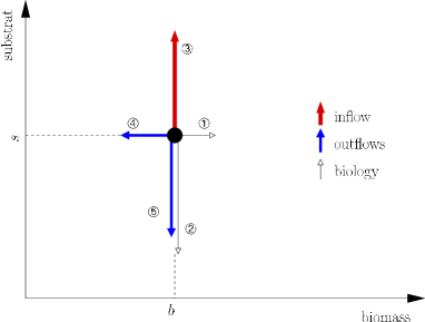
In view of (3), we are led to consider five jumps:

  • biology term: biomass increase of size ν1(x)subscript𝜈1𝑥\nu_{1}(x) at rate λ1(x)subscript𝜆1𝑥\lambda_{1}(x);

  • biology term: substrate decrease of size ν2(x)subscript𝜈2𝑥\nu_{2}(x) at rate λ2(x)subscript𝜆2𝑥\lambda_{2}(x);

  • inflow term: substrate inflow of size ν3(x)subscript𝜈3𝑥\nu_{3}(x) at rate λ3(x)subscript𝜆3𝑥\lambda_{3}(x);

  • outflow term: biomass outflow of size ν4(x)subscript𝜈4𝑥\nu_{4}(x) at rate λ4(x)subscript𝜆4𝑥\lambda_{4}(x);

  • outflow term: substrate outflow of size ν5(x)subscript𝜈5𝑥\nu_{5}(x) at rate λ5(x)subscript𝜆5𝑥\lambda_{5}(x);

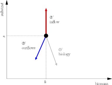
(see Figure 1). It remains to set the jump size rates so as to comply with the mass balance principle and the stochastic mass action law.

For a macroscopically infinitesimal ΔtΔ𝑡\Delta t, denote by ΔXtb,bioΔsubscriptsuperscript𝑋b,bio𝑡\Delta X^{\textrm{\tiny b,bio}}_{t}, ΔXts,bioΔsubscriptsuperscript𝑋s,bio𝑡\Delta X^{\textrm{\tiny s,bio}}_{t}, ΔXts,inΔsubscriptsuperscript𝑋s,in𝑡\Delta X^{\textrm{\tiny s,in}}_{t}, ΔXtb,outΔsubscriptsuperscript𝑋b,out𝑡\Delta X^{\textrm{\tiny b,out}}_{t}, ΔXts,bioΔsubscriptsuperscript𝑋s,bio𝑡\Delta X^{\textrm{\tiny s,bio}}_{t} the cumulated jump of type ➀, ➁, ➂, ➃, ➄ respectively, on state process Xtsubscript𝑋𝑡X_{t} within the time interval [t,t+Δt)𝑡𝑡Δ𝑡[t,t+\Delta t).

We first focus on the first two expressions. The stochastic mass action law [28] requires

𝔼[ΔXtb,bio|Xt=x]𝔼delimited-[]conditionalΔsubscriptsuperscript𝑋b,bio𝑡subscript𝑋𝑡𝑥\displaystyle\mathbb{E}[\Delta X^{\textrm{\tiny b,bio}}_{t}|X_{t}=x] (μ(s)bΔt0),similar-to-or-equalsabsent𝜇𝑠𝑏Δ𝑡0\displaystyle\simeq\left(\begin{smallmatrix}\mu(s)\,b\,\Delta t\\ 0\end{smallmatrix}\right)\,,
𝔼[ΔXts,bio|Xt=x]𝔼delimited-[]conditionalΔsubscriptsuperscript𝑋s,bio𝑡subscript𝑋𝑡𝑥\displaystyle\mathbb{E}[\Delta X^{\textrm{\tiny s,bio}}_{t}|X_{t}=x] (0kμ(s)bΔt).similar-to-or-equalsabsent0𝑘𝜇𝑠𝑏Δ𝑡\displaystyle\simeq\left(\begin{smallmatrix}0\\ -k\,\mu(s)\,b\,\Delta t\end{smallmatrix}\right)\,.

Now notice that, for small ΔtΔ𝑡\Delta t, the number of jumps of type ➀ (resp. ➁) within [t,t+Δt)𝑡𝑡Δ𝑡[t,t+\Delta t) is approximately 𝒫(λ1(x)Δt)𝒫subscript𝜆1𝑥Δ𝑡\mathcal{P}(\lambda_{1}(x)\,\Delta t) (resp. 𝒫(λ2(x)Δt)𝒫subscript𝜆2𝑥Δ𝑡\mathcal{P}(\lambda_{2}(x)\,\Delta t)), so that

𝔼[ΔXtb,bio|Xt=x]𝔼delimited-[]conditionalΔsubscriptsuperscript𝑋b,bio𝑡subscript𝑋𝑡𝑥\displaystyle\mathbb{E}[\Delta X^{\textrm{\tiny b,bio}}_{t}|X_{t}=x] λ1(x)Δtν1(x),similar-to-or-equalsabsentsubscript𝜆1𝑥Δ𝑡subscript𝜈1𝑥\displaystyle\simeq\lambda_{1}(x)\,\Delta t\,\nu_{1}(x)\,,
𝔼[ΔXts,bio|Xt=x]𝔼delimited-[]conditionalΔsubscriptsuperscript𝑋s,bio𝑡subscript𝑋𝑡𝑥\displaystyle\mathbb{E}[\Delta X^{\textrm{\tiny s,bio}}_{t}|X_{t}=x] λ2(x)Δtν2(x).similar-to-or-equalsabsentsubscript𝜆2𝑥Δ𝑡subscript𝜈2𝑥\displaystyle\simeq\lambda_{2}(x)\,\Delta t\,\nu_{2}(x)\,.

So we are looking for (λi(x),νi(x))subscript𝜆𝑖𝑥subscript𝜈𝑖𝑥(\lambda_{i}(x),\nu_{i}(x)) satisfying:

λ1(x)ν1(x)=(μ(s)b0) and λ2(x)ν2(x)=(0kμ(s)b).formulae-sequencesubscript𝜆1𝑥subscript𝜈1𝑥𝜇𝑠𝑏0 and subscript𝜆2𝑥subscript𝜈2𝑥0𝑘𝜇𝑠𝑏\displaystyle\lambda_{1}(x)\,\nu_{1}(x)=\left(\begin{smallmatrix}\mu(s)\,b\\ 0\end{smallmatrix}\right)\quad\textrm{ and }\quad\lambda_{2}(x)\,\nu_{2}(x)=\left(\begin{smallmatrix}0\\ -k\,\mu(s)\,b\end{smallmatrix}\right)\,. (8)

We therefore introduce the scale parameters K1subscript𝐾1K_{1} and K2subscript𝐾2K_{2} and we choose:

λ1(x)subscript𝜆1𝑥\displaystyle\lambda_{1}(x) =defK1μ(s)b,superscriptdefabsentsubscript𝐾1𝜇𝑠𝑏\displaystyle\stackrel{{\scriptstyle{\textrm{\rm\tiny def}}}}{{=}}K_{1}\,\mu(s)\,b\,, ν1subscript𝜈1\displaystyle\nu_{1} =def(1K10),superscriptdefabsent1subscript𝐾10\displaystyle\stackrel{{\scriptstyle{\textrm{\rm\tiny def}}}}{{=}}\left(\begin{smallmatrix}\frac{1}{K_{1}}\\ 0\end{smallmatrix}\right)\,,
λ2(x)subscript𝜆2𝑥\displaystyle\lambda_{2}(x) =defK2kμ(s)bsuperscriptdefabsentsubscript𝐾2𝑘𝜇𝑠𝑏\displaystyle\stackrel{{\scriptstyle{\textrm{\rm\tiny def}}}}{{=}}K_{2}\,k\,\mu(s)\,b ν2subscript𝜈2\displaystyle\nu_{2} =def(01K2).superscriptdefabsent01subscript𝐾2\displaystyle\stackrel{{\scriptstyle{\textrm{\rm\tiny def}}}}{{=}}-\left(\begin{smallmatrix}0\\ \frac{1}{K_{2}}\end{smallmatrix}\right)\,.

this choice is not unique and will be explain later in Section 3.5.

Here by “scale” we mean that jumps due to i will be of magnitude 1Ki1subscript𝐾𝑖\frac{1}{K_{i}} and the corresponding rates will be of magnitude Kisubscript𝐾𝑖K_{i}. Large Kisubscript𝐾𝑖K_{i} yields frequent and small jumps. Using the Poisson argument mentioned above, we see that these scale parameters Kisubscript𝐾𝑖K_{i} do not act on the mean values of the increments but on their variances (large Kisubscript𝐾𝑖K_{i} will correspond to small variances). The Kisubscript𝐾𝑖K_{i}’s can thus be regarded as tuning parameters quantifying the uncertainty or regularity of the corresponding source of variation.

Reproducing this discussion with the three other types of jumps, and considering only admissible jumps (in the positive orthant), we obtain a pure jump Markov process with rate coefficients λi(x)subscript𝜆𝑖𝑥\lambda_{i}(x) and associated jumps νi(x)subscript𝜈𝑖𝑥\nu_{i}(x) defined in Table 1.

biomass substrate substrate biomass substrate
increase decrease inflow outflow outflow
biology inflow outflow
rate λi(x)subscript𝜆𝑖𝑥\lambda_{i}(x) K1μ(s)bsubscript𝐾1𝜇𝑠𝑏K_{1}\,\mu(s)\,b K2kμ(s)bsubscript𝐾2𝑘𝜇𝑠𝑏K_{2}\,k\,\mu(s)\,b K3Dsinsubscript𝐾3𝐷superscript𝑠inK_{3}\,D\,s^{\textrm{\tiny in}} K4Dbsubscript𝐾4𝐷𝑏K_{4}\,D\,b K5Dssubscript𝐾5𝐷𝑠K_{5}\,D\,s \displaystyle\int
jump νi(x)subscript𝜈𝑖𝑥\nu_{i}(x) (1K10)matrix1subscript𝐾10\begin{pmatrix}\frac{1}{K_{1}}\\ 0\end{pmatrix} (01K2sK2)matrix01subscript𝐾2𝑠subscript𝐾2-\begin{pmatrix}0\\ \frac{1\wedge K_{2}\,s}{K_{2}}\end{pmatrix} (01K3)matrix01subscript𝐾3\begin{pmatrix}0\\ \frac{1}{K_{3}}\end{pmatrix} (1K4bK40)matrix1subscript𝐾4𝑏subscript𝐾40-\begin{pmatrix}\frac{1\wedge K_{4}\,b}{K_{4}}\\ 0\end{pmatrix} (01K5sK5)matrix01subscript𝐾5𝑠subscript𝐾5-\begin{pmatrix}0\\ \frac{1\wedge K_{5}\,s}{K_{5}}\end{pmatrix} (010)matrix010\begin{pmatrix}0\\ -1\\ 0\end{pmatrix}
Table 1: Rates and jumps of the five basic mechanisms of the pure jump process. Note that the jumps νi(x)subscript𝜈𝑖𝑥\nu_{i}(x) essentially do not depend on x𝑥x except for the negative jumps near the border {x=(b,s)+2;b=0 or s=0}formulae-sequence𝑥superscript𝑏𝑠subscriptsuperscript2𝑏0 or 𝑠0\{x=(b,s)^{*}\in\mathbb{R}^{2}_{+};b=0\textrm{ or }s=0\}.

About scales parameters

Let mbsubscript𝑚bm_{\textrm{\tiny b}} and mssubscript𝑚sm_{\textrm{\tiny s}} denote the representative masses of a single bacteria and of a single molecule of substrate. Typically mbmsmuch-greater-thansubscript𝑚bsubscript𝑚sm_{\textrm{\tiny b}}\gg m_{\textrm{\tiny s}} (e.g. mb106mssimilar-to-or-equalssubscript𝑚bsuperscript106subscript𝑚sm_{\textrm{\tiny b}}\simeq 10^{6}\,m_{\textrm{\tiny s}}). Hence:

0<Ki1mb,for i=1,4and0<Ki1ms,for i=2,3,5.formulae-sequence0subscript𝐾𝑖1subscript𝑚bformulae-sequencefor 𝑖14and0subscript𝐾𝑖1subscript𝑚sfor 𝑖235\displaystyle 0<K_{i}\leq\frac{1}{m_{\textrm{\tiny b}}}\,,\ \textrm{for }i=1,4\quad\textrm{and}\quad 0<K_{i}\leq\frac{1}{m_{\textrm{\tiny s}}}\,,\ \textrm{for }i=2,3,5\,.

In most cases KiKjmuch-less-thansubscript𝐾𝑖subscript𝐾𝑗K_{i}\ll K_{j} for i=1,4𝑖14i=1,4 and j=2,3,5𝑗235j=2,3,5, but it is possible to adjust the coefficients K𝐾K’s to the specific application considered. For example K2subscript𝐾2K_{2} will be large in laboratory experimental conditions, but for a real implementation the substrate inflow concentration could have a large variance. Also for the outflow, in regular conditions K4subscript𝐾4K_{4} and K5subscript𝐾5K_{5} could be large, but in bad mixing conditions they could be smaller. Finally K1subscript𝐾1K_{1} could be smaller than K4subscript𝐾4K_{4}, as the biomass concentration increase presents more variance than the substrate decrease (which is more regular as it is related to the diffusion of substrate across cell membranes).
Refer to caption
Figure 1: In this model, from a position x=(b,s)𝑥superscript𝑏𝑠x=(b,s)^{*} the process could jump according to 5 mechanisms (2 due to the biology, 1 inflow, and 2 outflows), the basic jump i has a length 1Ki1subscript𝐾𝑖\frac{1}{K_{i}} for i=1,,5𝑖15i=1,\dots,5.

As proved later in Lemma A.1, the jumps νi(x)subscript𝜈𝑖𝑥\nu_{i}(x) are essentially constant and equal to:

ν1subscript𝜈1\displaystyle\nu_{1} =def(1K10),superscriptdefabsentmatrix1subscript𝐾10\displaystyle\stackrel{{\scriptstyle{\textrm{\rm\tiny def}}}}{{=}}\begin{pmatrix}\frac{1}{K_{1}}\\ 0\end{pmatrix}\,, ν2subscript𝜈2\displaystyle\nu_{2} =def(01K2),superscriptdefabsentmatrix01subscript𝐾2\displaystyle\stackrel{{\scriptstyle{\textrm{\rm\tiny def}}}}{{=}}-\begin{pmatrix}0\\ \frac{1}{K_{2}}\end{pmatrix}\,, ν3subscript𝜈3\displaystyle\nu_{3} =def(01K3),superscriptdefabsentmatrix01subscript𝐾3\displaystyle\stackrel{{\scriptstyle{\textrm{\rm\tiny def}}}}{{=}}\begin{pmatrix}0\\ \frac{1}{K_{3}}\end{pmatrix}\,, ν4subscript𝜈4\displaystyle\nu_{4} =def(1K40),superscriptdefabsentmatrix1subscript𝐾40\displaystyle\stackrel{{\scriptstyle{\textrm{\rm\tiny def}}}}{{=}}-\begin{pmatrix}\frac{1}{K_{4}}\\ 0\end{pmatrix}\,, ν5subscript𝜈5\displaystyle\nu_{5} =def(01K5).superscriptdefabsentmatrix01subscript𝐾5\displaystyle\stackrel{{\scriptstyle{\textrm{\rm\tiny def}}}}{{=}}-\begin{pmatrix}0\\ \frac{1}{K_{5}}\end{pmatrix}\,. (9)

Representation of Xtsubscript𝑋𝑡X_{t}

The constructive description of the process Xtsubscript𝑋𝑡X_{t} that has been just presented would be used for simulation purposes, see Section 4.1. Nevertheless, it should be completed by a more comprehensible and synthetic representation. This will require some mathematical developments which we summarize now and that are detailed in Appendix A.

First we should notice that the jump process Xtsubscript𝑋𝑡X_{t} can be represented as the following (jump) SDE:

Xt=X0+i=15(0,t]×[0,)νi(Xu)missing1{vλi(Xu)}Ni(du×dv)subscript𝑋𝑡subscript𝑋0superscriptsubscript𝑖15subscript0𝑡0subscript𝜈𝑖subscript𝑋superscript𝑢subscriptmissing1𝑣subscript𝜆𝑖subscript𝑋superscript𝑢superscript𝑁𝑖d𝑢d𝑣\displaystyle X_{t}=X_{0}+\sum_{i=1}^{5}\int_{(0,t]\times[0,\infty)}\nu_{i}(X_{u^{-}})\,{\mathrm{\mathbf{missing}}1}_{\{v\leq\lambda_{i}(X_{u^{-}})\}}\,N^{i}({{\textrm{d}}}u\times{{\textrm{d}}}v) (10)

where Nisuperscript𝑁𝑖N^{i} are independent random Poisson measures with intensity measure du×dvd𝑢d𝑣{{\textrm{d}}}u\times{{\textrm{d}}}v (Lebesgue measure).

The process Xtsubscript𝑋𝑡X_{t} can be described as a Markov process with infinitesimal generator 𝒜ϕ(x)=limt01t[𝔼ϕ(Xtx)ϕ(x)]𝒜italic-ϕ𝑥subscript𝑡01𝑡delimited-[]𝔼italic-ϕsubscriptsuperscript𝑋𝑥𝑡italic-ϕ𝑥{\mathcal{A}}\phi(x)=\lim_{t\to 0}\frac{1}{t}\,[\mathbb{E}\phi(X^{x}_{t})-\phi(x)] where Xtxsubscriptsuperscript𝑋𝑥𝑡X^{x}_{t} is the process Xtsubscript𝑋𝑡X_{t} starting from x𝑥x. This operator completely characterizes the law of the process Xtsubscript𝑋𝑡X_{t}. In Appendix A we prove that this process is non explosive, i.e. it is defined for all t0𝑡0t\geq 0; that it admits moments as soon as X0subscript𝑋0X_{0} does; and that it is solution of (10) see Proposition A.3.

Still representation (10) is opaque. We can establish that the process Xtsubscript𝑋𝑡X_{t} essentially admits the following representation:

dBtdsubscript𝐵𝑡\displaystyle{{\textrm{d}}}B_{t} =(μ(St)BtDBt)dt+dm¯t1K1+dm¯t4K4,absent𝜇subscript𝑆𝑡subscript𝐵𝑡𝐷subscript𝐵𝑡d𝑡dsubscriptsuperscript¯𝑚1𝑡subscript𝐾1dsubscriptsuperscript¯𝑚4𝑡subscript𝐾4\displaystyle=\big{(}\mu(S_{t})\,B_{t}-D\,B_{t}\big{)}\,{{\textrm{d}}}t\textstyle+\frac{{{\textrm{d}}}\bar{m}^{1}_{t}}{\sqrt{K_{1}}}+\frac{{{\textrm{d}}}\bar{m}^{4}_{t}}{\sqrt{K_{4}}}\,, (11a)
dStdsubscript𝑆𝑡\displaystyle{{\textrm{d}}}S_{t} =(kμ(St)Bt+D(sinSt))dt+dm¯t2K2+dm¯t3K3+dm¯t5K5absent𝑘𝜇subscript𝑆𝑡subscript𝐵𝑡𝐷superscript𝑠insubscript𝑆𝑡d𝑡dsubscriptsuperscript¯𝑚2𝑡subscript𝐾2dsubscriptsuperscript¯𝑚3𝑡subscript𝐾3dsubscriptsuperscript¯𝑚5𝑡subscript𝐾5\displaystyle=\big{(}-k\,\mu(S_{t})\,B_{t}+D\,(s^{\textrm{\tiny in}}-S_{t})\big{)}\,{{\textrm{d}}}t\textstyle+\frac{{{\textrm{d}}}\bar{m}^{2}_{t}}{\sqrt{K_{2}}}+\frac{{{\textrm{d}}}\bar{m}^{3}_{t}}{\sqrt{K_{3}}}+\frac{{{\textrm{d}}}\bar{m}^{5}_{t}}{\sqrt{K_{5}}} (11b)

where m¯tisubscriptsuperscript¯𝑚𝑖𝑡\bar{m}^{i}_{t} are independent square integrable martingales with zero mean. The exact representation (41) differs from (11) only through terms (1Kis)1subscript𝐾𝑖𝑠(1\wedge K_{i}\,s) and (1Kib)1subscript𝐾𝑖𝑏(1\wedge K_{i}\,b) that are equal to 1 except on a very limited neighborhood of the axes.

The martingales m¯tisubscriptsuperscript¯𝑚𝑖𝑡\bar{m}^{i}_{t} are of mean 0 and they are explicitly known, see (40), as well as their quadratic variation, see (42). From Equation (11), the deterministic part of the process Xtsubscript𝑋𝑡X_{t}, its drift coefficient, appears to be essentially the classical ODE (1); and the stochastic part of this dynamics, the martingale terms, are of order 1/Ki1subscript𝐾𝑖1/\sqrt{K_{i}}.

3.2 Discrete time approximations

Poisson approximation X~tn=(B~tn,S~tn)subscript~𝑋subscript𝑡𝑛superscriptsubscript~𝐵subscript𝑡𝑛subscript~𝑆subscript𝑡𝑛\tilde{X}_{t_{n}}=(\tilde{B}_{t_{n}},\tilde{S}_{t_{n}})^{*}

For any small Δt>0Δ𝑡0\Delta t>0 given, let tn=nΔtsubscript𝑡𝑛𝑛Δ𝑡t_{n}=n\,\Delta t. We propose a discrete time Poisson approximation (X~tn)n0subscriptsubscript~𝑋subscript𝑡𝑛𝑛0(\tilde{X}_{t_{n}})_{n\geq 0} of (Xt)t0subscriptsubscript𝑋𝑡𝑡0(X_{t})_{t\geq 0}: on the interval [tn,tn+1)subscript𝑡𝑛subscript𝑡𝑛1[t_{n},t_{n+1}) we froze the rate functions λi(Xt)subscript𝜆𝑖subscript𝑋𝑡\lambda_{i}(X_{t}) to λi(Xtn)subscript𝜆𝑖subscript𝑋subscript𝑡𝑛\lambda_{i}(X_{t_{n}}) so that we get a Poisson distribution. The jumps νi(Xt)subscript𝜈𝑖subscript𝑋𝑡\nu_{i}(X_{t}) are also frozen to νi(Xtn)subscript𝜈𝑖subscript𝑋subscript𝑡𝑛\nu_{i}(X_{t_{n}}). Let X~0=X0subscript~𝑋0subscript𝑋0\tilde{X}_{0}=X_{0}, the approximation is defined by:

X~tn+1=X~tn+i=15νi(X~tn)𝒫ni(Δtλi(X~tn))subscript~𝑋subscript𝑡𝑛1subscript~𝑋subscript𝑡𝑛superscriptsubscript𝑖15subscript𝜈𝑖subscript~𝑋subscript𝑡𝑛superscriptsubscript𝒫𝑛𝑖Δ𝑡subscript𝜆𝑖subscript~𝑋subscript𝑡𝑛\displaystyle\tilde{X}_{t_{n+1}}=\tilde{X}_{t_{n}}+\sum_{i=1}^{5}\nu_{i}(\tilde{X}_{t_{n}})\,{\mathcal{P}}_{n}^{i}(\Delta t\,\lambda_{i}(\tilde{X}_{t_{n}})) (12)

where (𝒫ni(ρ))n,i=15subscriptsubscriptsuperscript𝒫𝑖𝑛𝜌formulae-sequence𝑛𝑖15({\mathcal{P}}^{i}_{n}(\rho))_{n\in\mathbb{N},i=1\cdots 5} are independent Poisson variables with intensities ρ𝜌\rho.

We have:

𝔼[X~tn+1|X~tn=x]𝔼delimited-[]conditionalsubscript~𝑋subscript𝑡𝑛1subscript~𝑋subscript𝑡𝑛𝑥\displaystyle\mathbb{E}[\tilde{X}_{t_{n+1}}|\tilde{X}_{t_{n}}=x] =x+i=15νi(x)𝔼[𝒫ni(Δtλi(X~tn))|X~tn=x]absent𝑥superscriptsubscript𝑖15subscript𝜈𝑖𝑥𝔼delimited-[]conditionalsuperscriptsubscript𝒫𝑛𝑖Δ𝑡subscript𝜆𝑖subscript~𝑋subscript𝑡𝑛subscript~𝑋subscript𝑡𝑛𝑥\displaystyle=x+\sum_{i=1}^{5}\nu_{i}(x)\,\mathbb{E}[{\mathcal{P}}_{n}^{i}(\Delta t\,\lambda_{i}(\tilde{X}_{t_{n}}))|\tilde{X}_{t_{n}}=x]
=x+Δti=15νi(x)λi(x)absent𝑥Δ𝑡superscriptsubscript𝑖15subscript𝜈𝑖𝑥subscript𝜆𝑖𝑥\displaystyle=x+\Delta t\,\sum_{i=1}^{5}\nu_{i}(x)\,\lambda_{i}(x) (13)

and let

fK(x)=defi=15νi(x)λi(x),superscriptdefsubscript𝑓𝐾𝑥superscriptsubscript𝑖15subscript𝜈𝑖𝑥subscript𝜆𝑖𝑥\displaystyle f_{K}(x)\stackrel{{\scriptstyle{\textrm{\rm\tiny def}}}}{{=}}\sum_{i=1}^{5}\nu_{i}(x)\,\lambda_{i}(x)\,, (14)

fK(x)subscript𝑓𝐾𝑥f_{K}(x) is “essentially” the r.h.s. function f(x)𝑓𝑥f(x) of the O.D.E. (1), more precisely fk(x)=f(x)subscript𝑓𝑘𝑥𝑓𝑥f_{k}(x)=f(x) except near the axes (see. Lemma A.1). In other words, the infinitesimal increments of the conditional mean follow the O.D.E. (1).

Also:

cov[X~tn+1|X~tn=x]covdelimited-[]conditionalsubscript~𝑋subscript𝑡𝑛1subscript~𝑋subscript𝑡𝑛𝑥\displaystyle\hbox{{{c}ov}}[\tilde{X}_{t_{n+1}}|\tilde{X}_{t_{n}}=x] =i=15cov[νi(x)𝒫ni(Δtλi(X~tn))|X~tn=x]=(Σ~1200Σ~22)absentsuperscriptsubscript𝑖15covdelimited-[]conditionalsubscript𝜈𝑖𝑥superscriptsubscript𝒫𝑛𝑖Δ𝑡subscript𝜆𝑖subscript~𝑋subscript𝑡𝑛subscript~𝑋subscript𝑡𝑛𝑥matrixsubscriptsuperscript~Σ2100subscriptsuperscript~Σ22\displaystyle=\sum_{i=1}^{5}\hbox{{{c}ov}}[\nu_{i}(x)\,{\mathcal{P}}_{n}^{i}(\Delta t\,\lambda_{i}(\tilde{X}_{t_{n}}))|\tilde{X}_{t_{n}}=x]=\begin{pmatrix}\tilde{\Sigma}^{2}_{1}&0\\ 0&\tilde{\Sigma}^{2}_{2}\end{pmatrix} (15a)
with
Σ~12subscriptsuperscript~Σ21\displaystyle\tilde{\Sigma}^{2}_{1} =1K12cov[𝒫n1(Δtλ1(x))]+1K42(1K4b)2cov[𝒫n4(Δtλ4(x))]absent1superscriptsubscript𝐾12covdelimited-[]superscriptsubscript𝒫𝑛1Δ𝑡subscript𝜆1𝑥1superscriptsubscript𝐾42superscript1subscript𝐾4𝑏2covdelimited-[]superscriptsubscript𝒫𝑛4Δ𝑡subscript𝜆4𝑥\displaystyle=\textstyle\frac{1}{K_{1}^{2}}\,\hbox{{{c}ov}}[{\mathcal{P}}_{n}^{1}(\Delta t\,\lambda_{1}(x))]+\frac{1}{K_{4}^{2}}\,(1\wedge K_{4}\,b)^{2}\,\hbox{{{c}ov}}[{\mathcal{P}}_{n}^{4}(\Delta t\,\lambda_{4}(x))]
=Δt{1K1μ(s)b+1K4(1K4b)2Db},absentΔ𝑡1subscript𝐾1𝜇𝑠𝑏1subscript𝐾4superscript1subscript𝐾4𝑏2𝐷𝑏\displaystyle\textstyle=\Delta t\,\Big{\{}\frac{1}{K_{1}}\,\mu(s)\,b+\frac{1}{K_{4}}\,(1\wedge K_{4}\,b)^{2}\,D\,b\Big{\}}\,, (15b)
Σ~22subscriptsuperscript~Σ22\displaystyle\tilde{\Sigma}^{2}_{2} =1K22(1K2s)2cov[𝒫n2(Δtλ2(x))]+1K32cov[𝒫n3(Δtλ3(x))]absent1superscriptsubscript𝐾22superscript1subscript𝐾2𝑠2covdelimited-[]superscriptsubscript𝒫𝑛2Δ𝑡subscript𝜆2𝑥1superscriptsubscript𝐾32covdelimited-[]superscriptsubscript𝒫𝑛3Δ𝑡subscript𝜆3𝑥\displaystyle=\textstyle\frac{1}{K_{2}^{2}}\,(1\wedge K_{2}\,s)^{2}\,\hbox{{{c}ov}}[{\mathcal{P}}_{n}^{2}(\Delta t\,\lambda_{2}(x))]+\frac{1}{K_{3}^{2}}\,\hbox{{{c}ov}}[{\mathcal{P}}_{n}^{3}(\Delta t\,\lambda_{3}(x))]
+1K52(1K5s)2cov[𝒫n5(Δtλ5(x))]1superscriptsubscript𝐾52superscript1subscript𝐾5𝑠2covdelimited-[]superscriptsubscript𝒫𝑛5Δ𝑡subscript𝜆5𝑥\displaystyle\qquad\qquad\qquad\qquad\qquad\qquad\textstyle+\frac{1}{K_{5}^{2}}\,(1\wedge K_{5}\,s)^{2}\,\hbox{{{c}ov}}[{\mathcal{P}}_{n}^{5}(\Delta t\,\lambda_{5}(x))]
=Δt{1K2(1K2s)2kμ(s)b+1K3Dsin+1K5(1K5s)2Ds}.absentΔ𝑡1subscript𝐾2superscript1subscript𝐾2𝑠2𝑘𝜇𝑠𝑏1subscript𝐾3𝐷superscript𝑠in1subscript𝐾5superscript1subscript𝐾5𝑠2𝐷𝑠\displaystyle\textstyle=\Delta t\,\Big{\{}\frac{1}{K_{2}}\,(1\wedge K_{2}\,s)^{2}\,k\,\mu(s)\,b+\frac{1}{K_{3}}\,D\,s^{\textrm{\tiny in}}+\frac{1}{K_{5}}\,(1\wedge K_{5}\,s)^{2}\,D\,s\Big{\}}\,. (15c)

Diffusion approximation ξ~tn=(β~tn,σ~tn)subscript~𝜉subscript𝑡𝑛superscriptsubscript~𝛽subscript𝑡𝑛subscript~𝜎subscript𝑡𝑛\tilde{\xi}_{t_{n}}=(\tilde{\beta}_{t_{n}},\tilde{\sigma}_{t_{n}})^{*}

In (12), the variable 𝒫ni(Δtλi(x))superscriptsubscript𝒫𝑛𝑖Δ𝑡subscript𝜆𝑖𝑥{\mathcal{P}}_{n}^{i}(\Delta t\,\lambda_{i}(x)) is Poisson distributed with parameter Δtλi(x)Δ𝑡subscript𝜆𝑖𝑥\Delta t\,\lambda_{i}(x). When this parameter is large (greater than 10 or 20) then this last distribution is very close to the normal distribution of mean Δtλi(x)Δ𝑡subscript𝜆𝑖𝑥\Delta t\,\lambda_{i}(x) and variance Δtλi(x)Δ𝑡subscript𝜆𝑖𝑥\Delta t\,\lambda_{i}(x). Hence, we get a (discrete time) normal approximation (ξ~tn)n0subscriptsubscript~𝜉subscript𝑡𝑛𝑛0(\tilde{\xi}_{t_{n}})_{n\geq 0} of (Xt)t0subscriptsubscript𝑋𝑡𝑡0(X_{t})_{t\geq 0} by letting ξ~0=X0subscript~𝜉0subscript𝑋0\tilde{\xi}_{0}=X_{0} and, conditionally on ξ~tn1=xsubscript~𝜉subscript𝑡𝑛1𝑥\tilde{\xi}_{t_{n-1}}=x:

ξ~tn+1=x+i=15νi(x)𝒩nisubscript~𝜉subscript𝑡𝑛1𝑥superscriptsubscript𝑖15subscript𝜈𝑖𝑥superscriptsubscript𝒩𝑛𝑖\displaystyle\tilde{\xi}_{t_{n+1}}=x+\sum_{i=1}^{5}\nu_{i}(x)\,{\mathcal{N}}_{n}^{i}

where 𝒩nisubscriptsuperscript𝒩𝑖𝑛{\mathcal{N}}^{i}_{n} are 5 independent Gaussian random variables :

𝒩ni𝒩(λi(x)Δt,λi(x)Δt)similar-tosubscriptsuperscript𝒩𝑖𝑛𝒩subscript𝜆𝑖𝑥Δ𝑡subscript𝜆𝑖𝑥Δ𝑡{\mathcal{N}}^{i}_{n}\sim{\mathcal{N}}\big{(}\lambda_{i}(x)\,\Delta t\,,\,\lambda_{i}(x)\,\Delta t\big{)}

So conditionally on ξ~tn=xsubscript~𝜉subscript𝑡𝑛𝑥\tilde{\xi}_{t_{n}}=x, ξ~tn+1subscript~𝜉subscript𝑡𝑛1\tilde{\xi}_{t_{n+1}} is normal with mean (13) and covariance matrix (15).

Let ξ~tn=(β~tn,σ~tn)subscript~𝜉subscript𝑡𝑛superscriptsubscript~𝛽subscript𝑡𝑛subscript~𝜎subscript𝑡𝑛\tilde{\xi}_{t_{n}}=(\tilde{\beta}_{t_{n}},\tilde{\sigma}_{t_{n}})^{*}, given β~tn=bsubscript~𝛽subscript𝑡𝑛𝑏\tilde{\beta}_{t_{n}}=b and σ~tn=ssubscript~𝜎subscript𝑡𝑛𝑠\tilde{\sigma}_{t_{n}}=s:

β~tn+1subscript~𝛽subscript𝑡𝑛1\displaystyle\tilde{\beta}_{t_{n+1}} =b+[μ(s)(1K4b)D]bΔt+Δtμ(s)bK1wn1+Δt(1K4b)2DbK4wn4absent𝑏delimited-[]𝜇𝑠1subscript𝐾4𝑏𝐷𝑏Δ𝑡Δ𝑡𝜇𝑠𝑏subscript𝐾1superscriptsubscript𝑤𝑛1Δ𝑡superscript1subscript𝐾4𝑏2𝐷𝑏subscript𝐾4superscriptsubscript𝑤𝑛4\displaystyle=b+\big{[}\mu(s)-(1\wedge K_{4}\,b)\,D\big{]}\,b\,\Delta t\textstyle+\sqrt{\Delta t\,\frac{\mu(s)\,b}{K_{1}}}\;w_{n}^{1}+\sqrt{\Delta t\,\frac{(1\wedge K_{4}\,b)^{2}\,D\,b}{K_{4}}}\;w_{n}^{4} (16a)
σ~tn+1subscript~𝜎subscript𝑡𝑛1\displaystyle\tilde{\sigma}_{t_{n+1}} =s+[(1K2s)kμ(s)b+Dsin(1K5s)Ds]Δtabsent𝑠delimited-[]1subscript𝐾2𝑠𝑘𝜇𝑠𝑏𝐷superscript𝑠in1subscript𝐾5𝑠𝐷𝑠Δ𝑡\displaystyle=s+\big{[}-(1\wedge K_{2}\,s)\,k\,\mu(s)\,b+D\,s^{\textrm{\tiny in}}-(1\wedge K_{5}\,s)\,D\,s\big{]}\,\Delta t
+Δt(1K2s)2kμ(s)bK2wn2+ΔtDsinK3wn3+Δt(1K5s)2DsK5wn5Δ𝑡superscript1subscript𝐾2𝑠2𝑘𝜇𝑠𝑏subscript𝐾2superscriptsubscript𝑤𝑛2Δ𝑡𝐷superscript𝑠insubscript𝐾3superscriptsubscript𝑤𝑛3Δ𝑡superscript1subscript𝐾5𝑠2𝐷𝑠subscript𝐾5superscriptsubscript𝑤𝑛5\displaystyle\quad\ \;\,+\textstyle\sqrt{\Delta t\,\frac{(1\wedge K_{2}\,s)^{2}\,k\,\mu(s)\,b}{K_{2}}}\;w_{n}^{2}+\sqrt{\Delta t\,\frac{D\,s^{\textrm{\tiny in}}}{K_{3}}}\;w_{n}^{3}+\sqrt{\Delta t\,\frac{(1\wedge K_{5}\,s)^{2}\,D\,s}{K_{5}}}\;w_{n}^{5} (16b)

where wnisubscriptsuperscript𝑤𝑖𝑛w^{i}_{n} are i.i.d. 𝒩(0,1)𝒩01{\mathcal{N}}(0,1) random variables.

Boundary conditions

In both approximations (12) and (16), no mechanism prevents the processes X~tnsubscript~𝑋subscript𝑡𝑛\tilde{X}_{t_{n}} or ξ~tnsubscript~𝜉subscript𝑡𝑛\tilde{\xi}_{t_{n}} from staying within the positive orthant +2subscriptsuperscript2\mathbb{R}^{2}_{+}. An ad hoc solution is to set the concentration to 0 whenever it becomes negative, see Section 4.

3.3 Diffusion model ξt=(βt,σt)subscript𝜉𝑡superscriptsubscript𝛽𝑡subscript𝜎𝑡\xi_{t}=(\beta_{t},\sigma_{t})^{*}

A stochastic differential equation model

System (16) is the Euler-Maruyama time discretization of the diffusion process ξt=(βt,σt)subscript𝜉𝑡superscriptsubscript𝛽𝑡subscript𝜎𝑡\xi_{t}=(\beta_{t},\sigma_{t})^{*} solution of the following SDE:

dβtdsubscript𝛽𝑡\displaystyle{{\textrm{d}}}\beta_{t} =[μ(σt)(1K4βt)D]βtdt+μ(σt)βtK1dWt1+(1K4βt)2DβtK4dWt4absentdelimited-[]𝜇subscript𝜎𝑡1subscript𝐾4subscript𝛽𝑡𝐷subscript𝛽𝑡d𝑡𝜇subscript𝜎𝑡subscript𝛽𝑡subscript𝐾1dsuperscriptsubscript𝑊𝑡1superscript1subscript𝐾4subscript𝛽𝑡2𝐷subscript𝛽𝑡subscript𝐾4dsuperscriptsubscript𝑊𝑡4\displaystyle=\big{[}\mu(\sigma_{t})-(1\wedge K_{4}\,\beta_{t})\,D\big{]}\,\beta_{t}\,{{\textrm{d}}}t\textstyle+\sqrt{\frac{\mu(\sigma_{t})\,\beta_{t}}{K_{1}}}\;{{\textrm{d}}}W_{t}^{1}+\sqrt{\frac{(1\wedge K_{4}\,\beta_{t})^{2}\,D\,\beta_{t}}{K_{4}}}\;{{\textrm{d}}}W_{t}^{4}
dσtdsubscript𝜎𝑡\displaystyle{{\textrm{d}}}\sigma_{t} =[(1K2σt)kμ(σt)βt+Dsin(1K5σt)Dσt]dtabsentdelimited-[]1subscript𝐾2subscript𝜎𝑡𝑘𝜇subscript𝜎𝑡subscript𝛽𝑡𝐷superscript𝑠in1subscript𝐾5subscript𝜎𝑡𝐷subscript𝜎𝑡d𝑡\displaystyle=\big{[}-(1\wedge K_{2}\,\sigma_{t})\,k\,\mu(\sigma_{t})\,\beta_{t}+D\,s^{\textrm{\tiny in}}-(1\wedge K_{5}\,\sigma_{t})\,D\,\sigma_{t}\big{]}\,{{\textrm{d}}}t
+(1K2σt)2kμ(σt)βtK2dWt2+DsinK3dWt3+(1K5σt)2DσtK5dWt5superscript1subscript𝐾2subscript𝜎𝑡2𝑘𝜇subscript𝜎𝑡subscript𝛽𝑡subscript𝐾2dsuperscriptsubscript𝑊𝑡2𝐷superscript𝑠insubscript𝐾3dsuperscriptsubscript𝑊𝑡3superscript1subscript𝐾5subscript𝜎𝑡2𝐷subscript𝜎𝑡subscript𝐾5dsuperscriptsubscript𝑊𝑡5\displaystyle\qquad+\textstyle\sqrt{\frac{(1\wedge K_{2}\,\sigma_{t})^{2}\,k\,\mu(\sigma_{t})\,\beta_{t}}{K_{2}}}\;{{\textrm{d}}}W_{t}^{2}+\sqrt{\frac{D\,s^{\textrm{\tiny in}}}{K_{3}}}\;{{\textrm{d}}}W_{t}^{3}+\sqrt{\frac{(1\wedge K_{5}\,\sigma_{t})^{2}\,D\,\sigma_{t}}{K_{5}}}\;{{\textrm{d}}}W_{t}^{5}

where Wtisubscriptsuperscript𝑊𝑖𝑡W^{i}_{t} are independent standard Wiener processes. Note that this result can be obtained directly from the process Xtsubscript𝑋𝑡X_{t} without the help of the discrete-time approximation. Indeed the infinitesimal generator of process Xtsubscript𝑋𝑡X_{t} given by (26) is a difference operator, and by Taylor development, it can be approximated by a second order differential operator corresponding to a diffusion process [6].

For small Kisubscript𝐾𝑖K_{i}’s the last system is equivalent considering:

dβtdsubscript𝛽𝑡\displaystyle{{\textrm{d}}}\beta_{t} =[μ(σt)βtDβt]dt+μ(σt)βtK1dWt1+DβtK4dWt4absentdelimited-[]𝜇subscript𝜎𝑡subscript𝛽𝑡𝐷subscript𝛽𝑡d𝑡𝜇subscript𝜎𝑡subscript𝛽𝑡subscript𝐾1dsuperscriptsubscript𝑊𝑡1𝐷subscript𝛽𝑡subscript𝐾4dsuperscriptsubscript𝑊𝑡4\displaystyle=\big{[}\mu(\sigma_{t})\,\beta_{t}-D\,\beta_{t}\big{]}\,{{\textrm{d}}}t\textstyle+\sqrt{\frac{\mu(\sigma_{t})\,\beta_{t}}{K_{1}}}\;{{\textrm{d}}}W_{t}^{1}+\sqrt{\frac{D\,\beta_{t}}{K_{4}}}\;{{\textrm{d}}}W_{t}^{4}
dσtdsubscript𝜎𝑡\displaystyle{{\textrm{d}}}\sigma_{t} =[kμ(σt)βt+DsinDσt]dtabsentdelimited-[]𝑘𝜇subscript𝜎𝑡subscript𝛽𝑡𝐷superscript𝑠in𝐷subscript𝜎𝑡d𝑡\displaystyle=\big{[}-k\,\mu(\sigma_{t})\,\beta_{t}+D\,s^{\textrm{\tiny in}}-D\,\sigma_{t}\big{]}\,{{\textrm{d}}}t
+kμ(σt)βtK2dWt2+DsinK3dWt3+DσtK5dWt5𝑘𝜇subscript𝜎𝑡subscript𝛽𝑡subscript𝐾2dsuperscriptsubscript𝑊𝑡2𝐷superscript𝑠insubscript𝐾3dsuperscriptsubscript𝑊𝑡3𝐷subscript𝜎𝑡subscript𝐾5dsuperscriptsubscript𝑊𝑡5\displaystyle\qquad\qquad\qquad+\textstyle\sqrt{\frac{k\,\mu(\sigma_{t})\,\beta_{t}}{K_{2}}}\;{{\textrm{d}}}W_{t}^{2}+\sqrt{\frac{D\,s^{\textrm{\tiny in}}}{K_{3}}}\;{{\textrm{d}}}W_{t}^{3}+\sqrt{\frac{D\,\sigma_{t}}{K_{5}}}\;{{\textrm{d}}}W_{t}^{5}

then we can group the Brownian motions in the following way:

dβtdsubscript𝛽𝑡\displaystyle{{\textrm{d}}}\beta_{t} =[μ(σt)D]βtdt+μ(σt)βtK1+DβtK4dWtbabsentdelimited-[]𝜇subscript𝜎𝑡𝐷subscript𝛽𝑡d𝑡𝜇subscript𝜎𝑡subscript𝛽𝑡subscript𝐾1𝐷subscript𝛽𝑡subscript𝐾4dsubscriptsuperscript𝑊b𝑡\displaystyle=\big{[}\mu(\sigma_{t})-D\big{]}\,\beta_{t}\,{{\textrm{d}}}t\textstyle+\sqrt{\frac{\mu(\sigma_{t})\,\beta_{t}}{K_{1}}+\frac{D\,\beta_{t}}{K_{4}}}\;{{\textrm{d}}}W^{\textrm{\tiny b}}_{t} (17a)
dσtdsubscript𝜎𝑡\displaystyle{{\textrm{d}}}\sigma_{t} =[kμ(σt)βt+D(sinσt)]dt+kμ(σt)βtK2+DsinK3+DσtK5dWtsabsentdelimited-[]𝑘𝜇subscript𝜎𝑡subscript𝛽𝑡𝐷superscript𝑠insubscript𝜎𝑡d𝑡𝑘𝜇subscript𝜎𝑡subscript𝛽𝑡subscript𝐾2𝐷superscript𝑠insubscript𝐾3𝐷subscript𝜎𝑡subscript𝐾5dsubscriptsuperscript𝑊s𝑡\displaystyle=\big{[}-k\,\mu(\sigma_{t})\,\beta_{t}+D\,(s^{\textrm{\tiny in}}-\sigma_{t})\big{]}\,{{\textrm{d}}}t+\textstyle\sqrt{\frac{k\,\mu(\sigma_{t})\,\beta_{t}}{K_{2}}+\frac{D\,s^{\textrm{\tiny in}}}{K_{3}}+\frac{D\,\sigma_{t}}{K_{5}}}\;{{\textrm{d}}}W^{\textrm{\tiny s}}_{t} (17b)

where Wbsuperscript𝑊bW^{\textrm{\tiny b}} and Wssuperscript𝑊sW^{\textrm{\tiny s}} are independent standard Wiener processes.

Behavior of the system of SDE’s near the axes

System (16) is the Euler-Maruyama time discretization of the SDE (17) (for large Kisubscript𝐾𝑖K_{i}’s). Even if the diffusion approximation is only valid for large values of the biomass and the substrate, we can study the behavior of (17) near the axes.

As for the discrete-time normal approximation, we should clarify the boundary conditions. As we well see, the component βtsubscript𝛽𝑡\beta_{t} given by (17a) will remain positive, but the component σtsubscript𝜎𝑡\sigma_{t} given by (17b) could become negative. We must first require that μ(s)=0𝜇𝑠0\mu(s)=0 for s<0𝑠0s<0. Then, note that each equation of (17) is related to the following well-known CIR model for interest rates:

Remark 3.1 (Cox-Ingersoll-Ross model)

Consider the one–dimensional SDE:

dXt=(a+bXt)dt+σXtdWt,X0=x00.formulae-sequencedsubscript𝑋𝑡𝑎𝑏subscript𝑋𝑡d𝑡𝜎subscript𝑋𝑡dsubscript𝑊𝑡subscript𝑋0subscript𝑥00\displaystyle{{\textrm{d}}}X_{t}=(a+b\,X_{t})\,{{\textrm{d}}}t+\sigma\,\sqrt{X_{t}}\,{{\textrm{d}}}W_{t}\,,\quad X_{0}=x_{0}\geq 0\,. (18)

with a0𝑎0a\geq 0, b𝑏b\in\mathbb{R}, σ>0𝜎0\sigma>0. According to [19, Prop. 6.2.4], for all x00subscript𝑥00x_{0}\geq 0, X𝑋X is a continuous process taking values in +superscript\mathbb{R}^{+}, and let τ=inf{t0,Xt=0}𝜏infimumformulae-sequence𝑡0subscript𝑋𝑡0\tau=\inf\{t\geq 0,\,X_{t}=0\}, then:

  1. (i)

    If aσ2/2𝑎superscript𝜎22a\geq\sigma^{2}/2, then τ=𝜏\tau=\infty xsubscript𝑥\mathbb{P}_{x}–a.s.;

  2. (ii)

    if 0a<σ2/20𝑎superscript𝜎220\leq a<\sigma^{2}/2 and b0𝑏0b\leq 0 then τ<𝜏\tau<\infty xsubscript𝑥\mathbb{P}_{x}–a.s.;

  3. (iii)

    if 0a<σ2/20𝑎superscript𝜎220\leq a<\sigma^{2}/2 and b>0𝑏0b>0 then x(τ<)(0,1)subscript𝑥𝜏01\mathbb{P}_{x}(\tau<\infty)\in(0,1).

In the first case, X𝑋X never reaches 0. In the second case X𝑋X a.s. reaches the state 0, in the third case it may reach 0. If a=0𝑎0a=0 then the state 0 is absorbing.

It is clear that β=0𝛽0\beta=0 is an absorbing state for (17a), and when β=0𝛽0\beta=0, (17b) reduces to

dσtdsubscript𝜎𝑡\displaystyle{{\textrm{d}}}\sigma_{t} =D(sinσt)dt+DsinK3+DσtK5dWtsabsent𝐷superscript𝑠insubscript𝜎𝑡d𝑡𝐷superscript𝑠insubscript𝐾3𝐷subscript𝜎𝑡subscript𝐾5dsubscriptsuperscript𝑊s𝑡\displaystyle=D\,(s^{\textrm{\tiny in}}-\sigma_{t})\,{{\textrm{d}}}t+\textstyle\sqrt{\frac{D\,s^{\textrm{\tiny in}}}{K_{3}}+\frac{D\,\sigma_{t}}{K_{5}}}\;{{\textrm{d}}}W^{\textrm{\tiny s}}_{t}

and from Remark 3.1, the solution of this SDE will stay on the half-line [K5K3sin,)subscript𝐾5subscript𝐾3superscript𝑠in[-\frac{K_{5}}{K_{3}}\,s^{\textrm{\tiny in}},\infty) and:

  1. (i)

    if sin(1K3+1K5)12K52superscript𝑠in1subscript𝐾31subscript𝐾512superscriptsubscript𝐾52s^{\textrm{\tiny in}}\,(\frac{1}{K_{3}}+\frac{1}{K_{5}})\geq\frac{1}{2\,K_{5}^{2}} then σtsubscript𝜎𝑡\sigma_{t} never reaches K5K3sinsubscript𝐾5subscript𝐾3superscript𝑠in-\frac{K_{5}}{K_{3}}\,s^{\textrm{\tiny in}};

  2. (ii)

    if sin(1K3+1K5)<12K52superscript𝑠in1subscript𝐾31subscript𝐾512superscriptsubscript𝐾52s^{\textrm{\tiny in}}\,(\frac{1}{K_{3}}+\frac{1}{K_{5}})<\frac{1}{2\,K_{5}^{2}} then σtsubscript𝜎𝑡\sigma_{t} reaches K5K3sinsubscript𝐾5subscript𝐾3superscript𝑠in-\frac{K_{5}}{K_{3}}\,s^{\textrm{\tiny in}} in finite time and is reflected.

Indeed, it is enough to apply Itô formula to σ~t=DsinK3+DσtK5subscript~𝜎𝑡𝐷superscript𝑠insubscript𝐾3𝐷subscript𝜎𝑡subscript𝐾5\tilde{\sigma}_{t}=\frac{D\,s^{\textrm{\tiny in}}}{K_{3}}+\frac{D\,\sigma_{t}}{K_{5}} and to use the Remark 3.1. Note that, as K5subscript𝐾5K_{5} is large, condition (i) is more realistic than condition (ii).

To extend the definition of (17) for negative value of σ𝜎\sigma, let suppose that μ(σ)=0𝜇𝜎0\mu(\sigma)=0 for σ0𝜎0\sigma\leq 0. As we seen, βtsubscript𝛽𝑡\beta_{t} will stay non-negative and β=0𝛽0\beta=0 is an absorbing state. Also σtK5K3sinsubscript𝜎𝑡subscript𝐾5subscript𝐾3superscript𝑠in\sigma_{t}\geq-\frac{K_{5}}{K_{3}}\,s^{\textrm{\tiny in}} and for large K5subscript𝐾5K_{5} this state will be repulsive. Note that for small values of σtsubscript𝜎𝑡\sigma_{t}, as the Kisubscript𝐾𝑖K_{i} are large, the diffusion term in (17b) will be small and the drift part will be dominated by Dsin𝐷superscript𝑠inD\,s^{\textrm{\tiny in}} so that σtsubscript𝜎𝑡\sigma_{t} will increase fast and its probability to be negative will be small.

The fact that the substrate concentration could be “negative” is due to the normal approximation. This approximation is valid for large values of concentration and the validity of the diffusion system (17) is questionable for small concentration. Nonetheless we can study its properties.

A possibility to get an SDE with positive solution is to consider an SDE with boundary condition [14, § IV-7] by adding a local time in {σ=0}𝜎0\{\sigma=0\} to the Equation (17b). This solution is rather artificial and will not be retained.

So the solution of the system (17) remains in the domain 𝒟=[0,)×[K5K3sin,)𝒟0subscript𝐾5subscript𝐾3superscript𝑠in{\mathcal{D}}=[0,\infty)\times[-\frac{K_{5}}{K_{3}}\,s^{\textrm{\tiny in}},\infty). The proof that this system admits a strong solution with pathwise uniqueness is presented in Appendix B.

3.4 Asymptotic analysis

The convergence of the pure jump model (10) or of the diffusion approximation (17) to the deterministic model (1) as all the Kisubscript𝐾𝑖K_{i}\to\infty can be rigorously established.

Let XtKsubscriptsuperscript𝑋𝐾𝑡X^{K}_{t} be the pure jump model defined at the beginning of Section 3.1, or as the solution of the Equation (10) for a given K=def(K1,K2,K3,K4,K5)superscriptdef𝐾subscript𝐾1subscript𝐾2subscript𝐾3subscript𝐾4subscript𝐾5K\stackrel{{\scriptstyle{\textrm{\rm\tiny def}}}}{{=}}(K_{1},K_{2},K_{3},K_{4},K_{5}). Let ξtKsubscriptsuperscript𝜉𝐾𝑡\xi^{K}_{t} be the solution of the SDE (17). Let x(t)𝑥𝑡x(t) be the EDO model solution of Equation (1). Then XtKsubscriptsuperscript𝑋𝐾𝑡X^{K}_{t} converges toward x(t)𝑥𝑡x(t) in the following way: for all T>0𝑇0T>0 and all δ>0𝛿0\delta>0,

(sup0tTXtKx(t)δ)0subscriptsupremum0𝑡𝑇normsubscriptsuperscript𝑋𝐾𝑡𝑥𝑡𝛿0\displaystyle\mathbb{P}\Big{(}\sup_{0\leq t\leq T}\left\|X^{K}_{t}-x(t)\right\|\geq\delta\Big{)}\longrightarrow 0 (19)

as Kisubscript𝐾𝑖K_{i}\to\infty for all i=15𝑖15i=1\cdots 5. This result is not surprising if we consider the representation (41) of (Xt)t0subscriptsubscript𝑋𝑡𝑡0(X_{t})_{t\geq 0}; it was obtained in a context of martingale convergence theorems in [17, 18] or in a more general context of convergence of sequences of infinitesimal generators in [6].

We can also prove the same type of convergence for the process ξtKsubscriptsuperscript𝜉𝐾𝑡\xi^{K}_{t}. Indeed, in Equation (17) the scale coefficients appears as 1/Ki1subscript𝐾𝑖1/\sqrt{K_{i}} in the diffusion part of the SDE, and the convergence clearly holds as all the Kisubscript𝐾𝑖K_{i} tends to infinity.

3.5 Other models

Refer to caption
Figure 2: In this simplified model, from a position x=(b,s)𝑥superscript𝑏𝑠x=(b,s)^{*} the process could jump according to 3 mechanisms (biology, inflow, and outflow), the basic jump isuperscripti\leavevmode\hbox to6.77pt{\vbox to6.77pt{\pgfpicture\makeatletter\hbox{\hskip 3.38579pt\lower-3.38579pt\hbox to0.0pt{\pgfsys@beginscope\pgfsys@invoke{ }\definecolor{pgfstrokecolor}{rgb}{0,0,0}\pgfsys@color@rgb@stroke{0}{0}{0}\pgfsys@invoke{ }\pgfsys@color@rgb@fill{0}{0}{0}\pgfsys@invoke{ }\pgfsys@setlinewidth{0.4pt}\pgfsys@invoke{ }\nullfont\hbox to0.0pt{\pgfsys@beginscope\pgfsys@invoke{ }{{}}\hbox{\hbox{{\pgfsys@beginscope\pgfsys@invoke{ }{{}{{{}}}{{}}{}{}{}{}{}{}{}{}{}{{}\pgfsys@moveto{3.18579pt}{0.0pt}\pgfsys@curveto{3.18579pt}{1.75948pt}{1.75948pt}{3.18579pt}{0.0pt}{3.18579pt}\pgfsys@curveto{-1.75948pt}{3.18579pt}{-3.18579pt}{1.75948pt}{-3.18579pt}{0.0pt}\pgfsys@curveto{-3.18579pt}{-1.75948pt}{-1.75948pt}{-3.18579pt}{0.0pt}{-3.18579pt}\pgfsys@curveto{1.75948pt}{-3.18579pt}{3.18579pt}{-1.75948pt}{3.18579pt}{0.0pt}\pgfsys@closepath\pgfsys@moveto{0.0pt}{0.0pt}\pgfsys@stroke\pgfsys@invoke{ } }{{{{}}\pgfsys@beginscope\pgfsys@invoke{ }\pgfsys@transformcm{1.0}{0.0}{0.0}{1.0}{-0.97221pt}{-2.3375pt}\pgfsys@invoke{ }\hbox{{\definecolor{pgfstrokecolor}{rgb}{0,0,0}\pgfsys@color@rgb@stroke{0}{0}{0}\pgfsys@invoke{ }\pgfsys@color@rgb@fill{0}{0}{0}\pgfsys@invoke{ }\hbox{{\it i\/}} }}\pgfsys@invoke{\lxSVG@closescope }\pgfsys@endscope}}} \pgfsys@invoke{\lxSVG@closescope }\pgfsys@endscope}}} \pgfsys@invoke{\lxSVG@closescope }\pgfsys@endscope{{{}}}{}{}\hss}\pgfsys@discardpath\pgfsys@invoke{\lxSVG@closescope }\pgfsys@endscope\hss}}\lxSVG@closescope\endpgfpicture}}\!\;^{\prime} has a length 1Ki1superscriptsubscript𝐾𝑖\frac{1}{K_{i}^{\prime}} for i=1,,3𝑖13i=1,\dots,3

As already noticed, the choice of (λi(x),νi(x))subscript𝜆𝑖𝑥subscript𝜈𝑖𝑥(\lambda_{i}(x),\nu_{i}(x)) satisfying (8) is not unique. We choose not to make the jump sizes depend on the state value x𝑥x (except for the boundary conditions), only the jump rates depend on x𝑥x. Another possibility is to choose jump sizes that depend on the state value x𝑥x. For example instead of the choice of Table 1, we can choose:

λ1(x)subscript𝜆1𝑥\displaystyle\lambda_{1}(x) =K1μ(s),absentsubscript𝐾1𝜇𝑠\displaystyle=K_{1}\,\mu(s)\,, λ2(x)subscript𝜆2𝑥\displaystyle\lambda_{2}(x) =K2kμ(s),absentsubscript𝐾2𝑘𝜇𝑠\displaystyle=K_{2}\,k\,\mu(s)\,, λ3(x)subscript𝜆3𝑥\displaystyle\lambda_{3}(x) =K3D,absentsubscript𝐾3𝐷\displaystyle=K_{3}\,D\,, λ4(x)subscript𝜆4𝑥\displaystyle\lambda_{4}(x) =K4D,absentsubscript𝐾4𝐷\displaystyle=K_{4}\,D\,, λ5(x)subscript𝜆5𝑥\displaystyle\lambda_{5}(x) =K5Dabsentsubscript𝐾5𝐷\displaystyle=K_{5}\,D

and

ν1(x)subscript𝜈1𝑥\displaystyle\nu_{1}(x) =(bK10),absent𝑏subscript𝐾10\displaystyle=\left(\begin{smallmatrix}\frac{b}{K_{1}}\\ 0\end{smallmatrix}\right)\,, ν2(x)subscript𝜈2𝑥\displaystyle\nu_{2}(x) =(0bK2),absent0𝑏subscript𝐾2\displaystyle=-\left(\begin{smallmatrix}0\\ \frac{b}{K_{2}}\end{smallmatrix}\right)\,, ν3(x)subscript𝜈3𝑥\displaystyle\nu_{3}(x) =(0sinK3),absent0superscript𝑠insubscript𝐾3\displaystyle=\left(\begin{smallmatrix}0\\ \frac{s^{\textrm{\tiny in}}}{K_{3}}\end{smallmatrix}\right)\,, ν4(x)subscript𝜈4𝑥\displaystyle\nu_{4}(x) =(bK40),absent𝑏subscript𝐾40\displaystyle=-\left(\begin{smallmatrix}\frac{b}{K_{4}}\\ 0\end{smallmatrix}\right)\,, ν5(x)subscript𝜈5𝑥\displaystyle\nu_{5}(x) =(0sK5)absent0𝑠subscript𝐾5\displaystyle=-\left(\begin{smallmatrix}0\\ \frac{s}{K_{5}}\end{smallmatrix}\right)

(if we neglect the boundary condition). Then in place of (17) we have the following set of equations:

dβtdsubscript𝛽𝑡\displaystyle{{\textrm{d}}}\beta_{t} =[μ(σt)βtDβt]dt+μ(σt)K1βtdWt1+DK4βtdWt4absentdelimited-[]𝜇subscript𝜎𝑡subscript𝛽𝑡𝐷subscript𝛽𝑡d𝑡𝜇subscript𝜎𝑡subscript𝐾1subscript𝛽𝑡dsuperscriptsubscript𝑊𝑡1𝐷subscript𝐾4subscript𝛽𝑡dsuperscriptsubscript𝑊𝑡4\displaystyle=\big{[}\mu(\sigma_{t})\,\beta_{t}-D\,\beta_{t}\big{]}\,{{\textrm{d}}}t\textstyle+\sqrt{\frac{\mu(\sigma_{t})}{K_{1}}}\,\beta_{t}\;{{\textrm{d}}}W_{t}^{1}+\sqrt{\frac{D}{K_{4}}}\,\beta_{t}\;{{\textrm{d}}}W_{t}^{4} (20a)
dσtdsubscript𝜎𝑡\displaystyle{{\textrm{d}}}\sigma_{t} =[kμ(σt)βt+DsinDσt]dtabsentdelimited-[]𝑘𝜇subscript𝜎𝑡subscript𝛽𝑡𝐷superscript𝑠in𝐷subscript𝜎𝑡d𝑡\displaystyle=\big{[}-k\,\mu(\sigma_{t})\,\beta_{t}+D\,s^{\textrm{\tiny in}}-D\,\sigma_{t}\big{]}\,{{\textrm{d}}}t
+kμ(σt)K2βtdWt2+DK3sindWt3+DK5σtdWt5𝑘𝜇subscript𝜎𝑡subscript𝐾2subscript𝛽𝑡dsuperscriptsubscript𝑊𝑡2𝐷subscript𝐾3superscript𝑠indsuperscriptsubscript𝑊𝑡3𝐷subscript𝐾5subscript𝜎𝑡dsuperscriptsubscript𝑊𝑡5\displaystyle\qquad\qquad\qquad+\textstyle\sqrt{\frac{k\,\mu(\sigma_{t})}{K_{2}}}\,\beta_{t}\;{{\textrm{d}}}W_{t}^{2}+\sqrt{\frac{D}{K_{3}}}\,s^{\textrm{\tiny in}}\;{{\textrm{d}}}W_{t}^{3}+\sqrt{\frac{D}{K_{5}}}\,\sigma_{t}\;{{\textrm{d}}}W_{t}^{5} (20b)

where Wisuperscript𝑊𝑖W^{i} are independent standard Wiener processes.

A three components model

Instead of the five components ➀ to ➄, we can consider a case with three independent sources of jump variation. This example strictly preserves the geometry (7) by considering three independent sources of jump variation:

  • biology term: biomass increase and substrate decrease at scale K1subscriptsuperscript𝐾1K^{\prime}_{1};

  • inflow term: substrate inflow at scale K2subscriptsuperscript𝐾2K^{\prime}_{2};

  • outflow term: biomass and substrate outflow at scale K3subscriptsuperscript𝐾3K^{\prime}_{3}

see Figure 2.

Again the jump sizes and rates should be chosen so as to satisfy the mass balance principle and the stochastic mass action, with no canonical choice. An ad hoc choice is given in the following table:

biology inflow outflow
rate λi(x)superscriptsubscript𝜆𝑖𝑥\lambda_{i}^{\prime}(x) K1μ(s)bsubscriptsuperscript𝐾1𝜇𝑠𝑏K^{\prime}_{1}\,\mu(s)\,b K2Dsubscriptsuperscript𝐾2𝐷K^{\prime}_{2}\,D K3Dsubscriptsuperscript𝐾3𝐷K^{\prime}_{3}\,D \displaystyle\int
jump νi(x)subscriptsuperscript𝜈𝑖𝑥\nu^{\prime}_{i}(x) (1K1kK1sK1)matrix1subscriptsuperscript𝐾1𝑘subscriptsuperscript𝐾1𝑠subscriptsuperscript𝐾1\begin{pmatrix}\frac{1}{K^{\prime}_{1}}\\[3.59995pt] -\frac{k\wedge K^{\prime}_{1}\,s}{K^{\prime}_{1}}\end{pmatrix} (0sinK2)matrix0superscript𝑠insubscriptsuperscript𝐾2\begin{pmatrix}0\\ \frac{s^{\textrm{\tiny in}}}{K^{\prime}_{2}}\end{pmatrix} (1K3xK3b1K3xK3s)matrix1subscriptsuperscript𝐾3norm𝑥subscriptsuperscript𝐾3𝑏1subscriptsuperscript𝐾3norm𝑥subscriptsuperscript𝐾3𝑠\begin{pmatrix}-\frac{1\wedge K^{\prime}_{3}\,\|x\|}{K^{\prime}_{3}}\,b\\[3.59995pt] -\frac{1\wedge K^{\prime}_{3}\,\|x\|}{K^{\prime}_{3}}\,s\end{pmatrix} (0100)matrix0100\begin{pmatrix}0\\ -1\\ 0\\ 0\end{pmatrix}
Table 2: Rates and jumps of an ad hoc choice for three mechanisms of the pure jump process. Note that the third jump ν3(x)subscriptsuperscript𝜈3𝑥\nu^{\prime}_{3}(x) is radial.

These jumps are now essentially equal to

ν1subscriptsuperscript𝜈1\displaystyle\nu^{\prime}_{1} =def1K1(1k),superscriptdefabsent1subscriptsuperscript𝐾1matrix1𝑘\displaystyle\stackrel{{\scriptstyle{\textrm{\rm\tiny def}}}}{{=}}\frac{1}{K^{\prime}_{1}}\,\begin{pmatrix}1\\ -k\end{pmatrix}\,, ν2subscriptsuperscript𝜈2\displaystyle\nu^{\prime}_{2} =def1K2(0sin),superscriptdefabsent1subscript𝐾2matrix0superscript𝑠in\displaystyle\stackrel{{\scriptstyle{\textrm{\rm\tiny def}}}}{{=}}\frac{1}{K_{2}}\begin{pmatrix}0\\ s^{\textrm{\tiny in}}\end{pmatrix}\,, ν3subscriptsuperscript𝜈3\displaystyle\nu^{\prime}_{3} =def1K3(bs).superscriptdefabsent1subscriptsuperscript𝐾3matrix𝑏𝑠\displaystyle\stackrel{{\scriptstyle{\textrm{\rm\tiny def}}}}{{=}}\frac{1}{K^{\prime}_{3}}\begin{pmatrix}-b\\ -s\end{pmatrix}.

This setting forces the jumps to be directed along the corresponding vector field, which is a strong constraint. In particular, the stoichiometry is strictly respected: the production of 1 unit of biomass requires exactly k𝑘k units of substrate. Moreover the outflow jump is always radial, so that the increments of biomass and substrate are again strongly linked. Notice that for this particular choice of λ3subscriptsuperscript𝜆3\lambda^{\prime}_{3} and ν3subscriptsuperscript𝜈3\nu^{\prime}_{3}, the jump rate is constant but the jump size is not. In other words, the jump carries information both in the direction and the intensity of the variation. This will affect the qualitative behavior of the process and of its diffusion approximation, regarding extinction for example.

As for our canonical model, we obtain a SDE for the diffusion approximation of the jump process :

dβtdsubscript𝛽𝑡\displaystyle{{\textrm{d}}}\beta_{t} =[μ(σt)(1K3βt)D]βtdt+μ(σt)βtK1dWt1+DK3(1K3ξt)βtdWt3absentdelimited-[]𝜇subscript𝜎𝑡1subscriptsuperscript𝐾3subscript𝛽𝑡𝐷subscript𝛽𝑡d𝑡𝜇subscript𝜎𝑡subscript𝛽𝑡subscriptsuperscript𝐾1dsuperscriptsubscript𝑊𝑡1𝐷subscriptsuperscript𝐾31subscriptsuperscript𝐾3normsubscript𝜉𝑡subscript𝛽𝑡dsuperscriptsubscript𝑊𝑡3\displaystyle=\big{[}\mu(\sigma_{t})-(1\wedge K^{\prime}_{3}\,\beta_{t})\,D\big{]}\,\beta_{t}\,{{\textrm{d}}}t\textstyle+\sqrt{\frac{\mu(\sigma_{t})\,\beta_{t}}{K^{\prime}_{1}}}\;{{\textrm{d}}}W_{t}^{1}+\sqrt{\frac{D}{K^{\prime}_{3}}}(1\wedge K^{\prime}_{3}\,\|\xi_{t}\|)\,\,\beta_{t}\;{{\textrm{d}}}W_{t}^{3}
dσtdsubscript𝜎𝑡\displaystyle{{\textrm{d}}}\sigma_{t} =[(kK1σt)μ(σt)βt+Dsin(1K3ξt)Dσt]dtabsentdelimited-[]𝑘subscriptsuperscript𝐾1subscript𝜎𝑡𝜇subscript𝜎𝑡subscript𝛽𝑡𝐷superscript𝑠in1subscriptsuperscript𝐾3normsubscript𝜉𝑡𝐷subscript𝜎𝑡d𝑡\displaystyle=\big{[}-(k\wedge K^{\prime}_{1}\,\sigma_{t})\,\mu(\sigma_{t})\,\beta_{t}+D\,s^{\textrm{\tiny in}}-(1\wedge K^{\prime}_{3}\,\|\xi_{t}\|)\,D\,\sigma_{t}\big{]}\,{{\textrm{d}}}t
+μ(σt)βtK2(kK1σt)dWt1+DK2sindWt2+DK3(1K3ξt)σtdWt5.𝜇subscript𝜎𝑡subscript𝛽𝑡subscript𝐾2𝑘subscriptsuperscript𝐾1subscript𝜎𝑡dsuperscriptsubscript𝑊𝑡1𝐷subscriptsuperscript𝐾2superscript𝑠indsuperscriptsubscript𝑊𝑡2𝐷subscriptsuperscript𝐾31subscriptsuperscript𝐾3normsubscript𝜉𝑡subscript𝜎𝑡dsuperscriptsubscript𝑊𝑡5\displaystyle\qquad+\textstyle\sqrt{\frac{\mu(\sigma_{t})\,\beta_{t}}{K_{2}}}\,(k\wedge K^{\prime}_{1}\,\sigma_{t})\;{{\textrm{d}}}W_{t}^{1}+\sqrt{\frac{D}{K^{\prime}_{2}}}\,s^{\textrm{\tiny in}}\;{{\textrm{d}}}W_{t}^{2}+\sqrt{\frac{D}{K^{\prime}_{3}}}\,(1\wedge K^{\prime}_{3}\,\|\xi_{t}\|)\,\,\sigma_{t}\;{{\textrm{d}}}W_{t}^{5}\ .

Notice that since W1superscript𝑊1W^{1} and W3superscript𝑊3W^{3} affect both components of ξtsubscript𝜉𝑡\xi_{t}, the quadratic variation process ξtsubscriptdelimited-⟨⟩𝜉𝑡\langle\xi\rangle_{t} will not be a diagonal matrix. In comparison with (7), we write the vector form of the SDE for large Kisubscript𝐾𝑖K_{i}’s:

d(βtσt)=[μ(σt)βt(1k)biology+D(0sin)inflowD(βtσt)outflow]dt+μ(σt)βtK1(1k)dWt1biology+DK2(0sin)dWt2inflow+DK3(βtσt)dWt3outflow.dsubscript𝛽𝑡subscript𝜎𝑡delimited-[]subscript𝜇subscript𝜎𝑡subscript𝛽𝑡1𝑘biologysubscript𝐷0superscript𝑠ininflowsubscript𝐷subscript𝛽𝑡subscript𝜎𝑡outflowd𝑡subscript𝜇subscript𝜎𝑡subscript𝛽𝑡subscriptsuperscript𝐾11𝑘dsuperscriptsubscript𝑊𝑡1biologysubscript𝐷subscriptsuperscript𝐾20superscript𝑠indsuperscriptsubscript𝑊𝑡2inflowsubscript𝐷subscriptsuperscript𝐾3subscript𝛽𝑡subscript𝜎𝑡dsuperscriptsubscript𝑊𝑡3outflow{{\textrm{d}}}\left(\begin{smallmatrix}\beta_{t}\\ \sigma_{t}\end{smallmatrix}\right)=\Big{[}\underbrace{\mu(\sigma_{t})\,\beta_{t}\,\left(\begin{smallmatrix}1\\ -k\\ \end{smallmatrix}\right)}_{\textrm{biology}}\underbrace{+D\,\left(\begin{smallmatrix}0\\ s^{\textrm{\tiny in}}\end{smallmatrix}\right)}_{\textrm{inflow}}\underbrace{-D\,\left(\begin{smallmatrix}\beta_{t}\\ \sigma_{t}\end{smallmatrix}\right)}_{\textrm{outflow}}\Big{]}\;{{\textrm{d}}}t\\ +\underbrace{\textstyle\sqrt{\frac{\mu(\sigma_{t})\,\beta_{t}}{K^{\prime}_{1}}}\left(\begin{smallmatrix}1\\ -k\end{smallmatrix}\right)\;{{\textrm{d}}}W_{t}^{1}}_{\textrm{biology}}+\underbrace{\textstyle\sqrt{\frac{D}{K^{\prime}_{2}}}\,\left(\begin{smallmatrix}0\\ s^{\textrm{\tiny in}}\end{smallmatrix}\right)\;{{\textrm{d}}}W_{t}^{2}}_{\textrm{inflow}}+\underbrace{\textstyle\sqrt{\frac{D}{K^{\prime}_{3}}}\,\left(\begin{smallmatrix}\beta_{t}\\ \sigma_{t}\end{smallmatrix}\right)\;{{\textrm{d}}}W_{t}^{3}}_{\textrm{outflow}}\ .

The diffusion term appears as the conjunction of three perturbations acting along the three vector fields determined by the sources of variation. Moreover, the intensity of the noise could be different for each type of perturbation. Considering this model could therefore be of interest, if the geometric interpretation of the noise is meaningful, see [16].

Comparison with the Imhof-Walcher model [15]

We finally mention that the diffusion model appearing in [15], is obtained from (20) by letting K1=K2=K3=0subscript𝐾1subscript𝐾2subscript𝐾30K_{1}=K_{2}=K_{3}=0 which leads to:

dβtdsubscript𝛽𝑡\displaystyle{{\textrm{d}}}\beta_{t} =[μ(σt)D]βtdt+cbβtdWtbabsentdelimited-[]𝜇subscript𝜎𝑡𝐷subscript𝛽𝑡d𝑡superscript𝑐bsubscript𝛽𝑡dsubscriptsuperscript𝑊b𝑡\displaystyle=\big{[}\mu(\sigma_{t})-D\big{]}\,\beta_{t}\,{{\textrm{d}}}t\textstyle+c^{\textrm{\tiny b}}\,\beta_{t}\;{{\textrm{d}}}W^{\textrm{\tiny b}}_{t} (21a)
dσtdsubscript𝜎𝑡\displaystyle{{\textrm{d}}}\sigma_{t} =[kμ(σt)βt+D(sinσt)]dt+csσtdWtsabsentdelimited-[]𝑘𝜇subscript𝜎𝑡subscript𝛽𝑡𝐷superscript𝑠insubscript𝜎𝑡d𝑡superscript𝑐ssubscript𝜎𝑡dsubscriptsuperscript𝑊s𝑡\displaystyle=\big{[}-k\,\mu(\sigma_{t})\,\beta_{t}+D\,(s^{\textrm{\tiny in}}-\sigma_{t})\big{]}\,{{\textrm{d}}}t+c^{\textrm{\tiny s}}\,\sigma_{t}\;{{\textrm{d}}}W^{\textrm{\tiny s}}_{t} (21b)

The choice of these coefficients is justified in [15] by constructing an approximating Markov chain, and then taking the limit as the sampling rate goes to 0. This model will be compared to the diffusion approximation (17) model on a simulation test in Section 5.4.

4 Simulation algorithms

We presented several models for the chemostat system: the pure jump model (Xt)t0subscriptsubscript𝑋𝑡𝑡0(X_{t})_{t\geq 0} could be considered as a detailed model at the microscopic scale. The Poisson approximation (X~tn)nsubscriptsubscript~𝑋subscript𝑡𝑛𝑛(\tilde{X}_{t_{n}})_{n\in\mathbb{N}} given by (12) and the normal approximation (ξ~tn)nsubscriptsubscript~𝜉subscript𝑡𝑛𝑛(\tilde{\xi}_{t_{n}})_{n\in\mathbb{N}} given (16) are constant time step approximation of the pure jump process. Finally the diffusion process (ξt)t0subscriptsubscript𝜉𝑡𝑡0(\xi_{t})_{t\geq 0} solution of the SDE (17) is a continuous time approximation of the pure jump process.

The now present the three associated simulation algorithms that will be valid at different scales.

4.1 Pure jump model

The pure jump model in continuous time described in Section 3.1 can be exactly simulated thanks to the Gillespie algorithm, also called stochastic simulation algorithm, described in Algorithm 1.


  t0𝑡0t\leftarrow 0, xx0𝑥subscript𝑥0x\leftarrow x_{0}
  save (t,x)𝑡𝑥(t,x)
  while tTmax𝑡superscript𝑇maxt\leq T^{\textrm{\tiny max}} do
     compute λi(x)subscript𝜆𝑖𝑥\lambda_{i}(x)% see Table 1
     λ=i=15λi(x)𝜆superscriptsubscript𝑖15subscript𝜆𝑖𝑥\lambda=\sum_{i=1}^{5}\lambda_{i}(x)
     ΔtExp(λ)similar-toΔ𝑡Exp𝜆\Delta t\sim\textrm{\rm Exp}(\lambda)% exponential distribution
     uU[0,1]similar-to𝑢U01u\sim\textrm{\rm U}[0,1]% uniform distribution
     tt+Δt𝑡𝑡Δ𝑡t\leftarrow t+\Delta t
     if uλ1(x)/λ𝑢subscript𝜆1𝑥𝜆u\leq\lambda_{1}(x)/\lambda then
        xx+ν¯1𝑥𝑥subscript¯𝜈1x\leftarrow x+\bar{\nu}_{1}% biomass reproduction
     else if u{λ1(x)+λ2(x)}/λ𝑢subscript𝜆1𝑥subscript𝜆2𝑥𝜆u\leq\{\lambda_{1}(x)+\lambda_{2}(x)\}/\lambda then
        x[xν¯2]+𝑥subscriptdelimited-[]𝑥subscript¯𝜈2x\leftarrow[x-\bar{\nu}_{2}]_{+}% consumption
     else if u{λ1(x)+λ2(x)+λ3(x)}/λ𝑢subscript𝜆1𝑥subscript𝜆2𝑥subscript𝜆3𝑥𝜆u\leq\{\lambda_{1}(x)+\lambda_{2}(x)+\lambda_{3}(x)\}/\lambda then
        xx+ν¯3𝑥𝑥subscript¯𝜈3x\leftarrow x+\bar{\nu}_{3}% substrate inflow
     else if u{λ1(x)+λ2(x)+λ3(x)+λ4(x)}/λ𝑢subscript𝜆1𝑥subscript𝜆2𝑥subscript𝜆3𝑥subscript𝜆4𝑥𝜆u\leq\{\lambda_{1}(x)+\lambda_{2}(x)+\lambda_{3}(x)+\lambda_{4}(x)\}/\lambda then
        x[xν¯4]+𝑥subscriptdelimited-[]𝑥subscript¯𝜈4x\leftarrow[x-\bar{\nu}_{4}]_{+}% biomass outflow
     else
        x[xν¯5]+𝑥subscriptdelimited-[]𝑥subscript¯𝜈5x\leftarrow[x-\bar{\nu}_{5}]_{+}% substrate outflow
     end if
     save (t,x)𝑡𝑥(t,x)
  end while

  Here ν¯1=(1/K10),subscript¯𝜈11subscript𝐾10\bar{\nu}_{1}=\big{(}\begin{smallmatrix}1/K_{1}\\ 0\end{smallmatrix}\big{)}, ν¯2=(01/K2),subscript¯𝜈201subscript𝐾2\bar{\nu}_{2}=\big{(}\begin{smallmatrix}0\\ 1/K_{2}\end{smallmatrix}\big{)}, ν¯3=(01/K3),subscript¯𝜈301subscript𝐾3\bar{\nu}_{3}=\big{(}\begin{smallmatrix}0\\ 1/K_{3}\end{smallmatrix}\big{)}, ν¯4=(1/K40),subscript¯𝜈41subscript𝐾40\bar{\nu}_{4}=\big{(}\begin{smallmatrix}1/K_{4}\\ 0\end{smallmatrix}\big{)}, ν¯5=(01/K5)subscript¯𝜈501subscript𝐾5\bar{\nu}_{5}=\big{(}\begin{smallmatrix}0\\ 1/K_{5}\end{smallmatrix}\big{)} and [x]+subscriptdelimited-[]𝑥[x]_{+} is the projection on the positive quadrant: [x]+=[(βσ)]+=(β0σ0)subscriptdelimited-[]𝑥subscriptdelimited-[]𝛽𝜎𝛽0𝜎0[x]_{+}=\left[\left(\begin{smallmatrix}\beta\\ \sigma\end{smallmatrix}\right)\right]_{+}=\left(\begin{smallmatrix}\beta\vee 0\\ \sigma\vee 0\end{smallmatrix}\right).

Algorithm 1: Gillespie algorithm (or stochastic simulation algorithm).

When the rate coefficients λi(x)subscript𝜆𝑖𝑥\lambda_{i}(x) are large the time increment will be small and the Gillespie algorithm is impractical. As the scale coefficients Kisubscript𝐾𝑖K_{i} are large, the λi(x)subscript𝜆𝑖𝑥\lambda_{i}(x), i3𝑖3i\neq 3, are large only when β𝛽\beta and σ𝜎\sigma are small; λ3(x)subscript𝜆3𝑥\lambda_{3}(x) will remain large as it does not depend on x𝑥x.

4.2 Poisson approximation


  t0𝑡0t\leftarrow 0, xx0𝑥subscript𝑥0x\leftarrow x_{0}
  save (t,x)𝑡𝑥(t,x)
  while tTmax𝑡superscript𝑇maxt\leq T^{\textrm{\tiny max}} do
     compute λi(x)subscript𝜆𝑖𝑥\lambda_{i}(x)% see Table 1
     λ=i=15λi(x)𝜆superscriptsubscript𝑖15subscript𝜆𝑖𝑥\lambda=\sum_{i=1}^{5}\lambda_{i}(x)
     compute 𝒎i(x)subscript𝒎𝑖𝑥\boldsymbol{m}_{i}(x), 𝒗i(x)subscript𝒗𝑖𝑥\boldsymbol{v}_{i}(x)% see (23)
     Δtmini=15{ελ/|𝒎i(x)|,ε2λ2/𝒗i(x)}Δ𝑡subscript𝑖15𝜀𝜆subscript𝒎𝑖𝑥superscript𝜀2superscript𝜆2subscript𝒗𝑖𝑥\Delta t\leftarrow\min_{i=1\cdots 5}\big{\{}\varepsilon\,\lambda/|\boldsymbol{m}_{i}(x)|\,,\,\varepsilon^{2}\,\lambda^{2}/\boldsymbol{v}_{i}(x)\big{\}}
     tt+Δt𝑡𝑡Δ𝑡t\leftarrow t+\Delta t
     𝒫iPoisson(λi(x)Δt)similar-tosubscript𝒫𝑖Poissonsubscript𝜆𝑖𝑥Δ𝑡{\mathcal{P}}_{i}\sim\textrm{Poisson}(\lambda_{i}(x)\,\Delta t) for i=15𝑖15i=1\cdots 5
     x[x+ν¯1𝒫1ν¯2𝒫2+ν¯3𝒫3ν¯4𝒫4ν¯5𝒫5]+𝑥subscriptdelimited-[]𝑥subscript¯𝜈1subscript𝒫1subscript¯𝜈2subscript𝒫2subscript¯𝜈3subscript𝒫3subscript¯𝜈4subscript𝒫4subscript¯𝜈5subscript𝒫5x\leftarrow[x+\bar{\nu}_{1}\,{\mathcal{P}}_{1}-\bar{\nu}_{2}\,{\mathcal{P}}_{2}+\bar{\nu}_{3}\,{\mathcal{P}}_{3}-\bar{\nu}_{4}\,{\mathcal{P}}_{4}-\bar{\nu}_{5}\,{\mathcal{P}}_{5}]_{+}
     save (t,x)𝑡𝑥(t,x)
  end while

  Here ν¯1=(1/K10),subscript¯𝜈11subscript𝐾10\bar{\nu}_{1}=\big{(}\begin{smallmatrix}1/K_{1}\\ 0\end{smallmatrix}\big{)}, ν¯2=(01/K2),subscript¯𝜈201subscript𝐾2\bar{\nu}_{2}=\big{(}\begin{smallmatrix}0\\ 1/K_{2}\end{smallmatrix}\big{)}, ν¯3=(01/K3),subscript¯𝜈301subscript𝐾3\bar{\nu}_{3}=\big{(}\begin{smallmatrix}0\\ 1/K_{3}\end{smallmatrix}\big{)}, ν¯4=(1/K40),subscript¯𝜈41subscript𝐾40\bar{\nu}_{4}=\big{(}\begin{smallmatrix}1/K_{4}\\ 0\end{smallmatrix}\big{)}, ν¯5=(01/K5)subscript¯𝜈501subscript𝐾5\bar{\nu}_{5}=\big{(}\begin{smallmatrix}0\\ 1/K_{5}\end{smallmatrix}\big{)} and [x]+subscriptdelimited-[]𝑥[x]_{+} is the projection on the positive quadrant: [x]+=[(βσ)]+=(β0σ0)subscriptdelimited-[]𝑥subscriptdelimited-[]𝛽𝜎𝛽0𝜎0[x]_{+}=\left[\left(\begin{smallmatrix}\beta\\ \sigma\end{smallmatrix}\right)\right]_{+}=\left(\begin{smallmatrix}\beta\vee 0\\ \sigma\vee 0\end{smallmatrix}\right).

Algorithm 2: Poisson approximation or tau-leap method.

The simulation of the previous model could be cumbersome for very high rates of event. In this case it is desirable to use the fixed time step Poisson approximation method (12) also called tau-leap [9]. Recently many papers have addressed the numerical analysis of this approximation scheme [23, 20, 1]. In this method the time step should be small enough so that it fulfills the following “leap condition”: the state change in any leap should be small enough that no rate function λi(x)subscript𝜆𝑖𝑥\lambda_{i}(x) will experience a macroscopically significant change in its value, that is:

|λi(x+iνi(x)𝒫ni(Δtλi(x)))λi(x)|ελ(x)subscript𝜆𝑖𝑥subscriptsuperscript𝑖subscript𝜈superscript𝑖𝑥subscriptsuperscript𝒫superscript𝑖𝑛Δ𝑡subscript𝜆superscript𝑖𝑥subscript𝜆𝑖𝑥𝜀𝜆𝑥\displaystyle\textstyle\Big{|}\lambda_{i}\big{(}x+\sum_{i^{\prime}}\nu_{i^{\prime}}(x)\,{\mathcal{P}}^{i^{\prime}}_{n}(\Delta t\,\lambda_{i^{\prime}}(x))\big{)}-\lambda_{i}(x)\Big{|}\leq\varepsilon\,\lambda(x) (22)

for i=15𝑖15i=1\cdots 5, where 0<ε10𝜀much-less-than10<\varepsilon\ll 1 is an error control parameter.

For this method to be practicable [10] proposed an automatic and simple way of determining the largest time step ΔtΔ𝑡\Delta t compatible with the leap condition. Define:

𝒎i(x)subscript𝒎𝑖𝑥\displaystyle\boldsymbol{m}_{i}(x) =defi=15λi(x)(λi(x)νi),superscriptdefabsentsuperscriptsubscriptsuperscript𝑖15subscript𝜆superscript𝑖𝑥subscript𝜆𝑖𝑥subscript𝜈superscript𝑖\displaystyle\stackrel{{\scriptstyle{\textrm{\rm\tiny def}}}}{{=}}\sum_{i^{\prime}=1}^{5}\lambda_{i^{\prime}}(x)\,\big{(}\nabla\lambda_{i}(x)\cdot\nu_{i^{\prime}}\big{)}\,, (23a)
𝒗i(x)subscript𝒗𝑖𝑥\displaystyle\boldsymbol{v}_{i}(x) =defi=15λi(x)(λi(x)νi)2superscriptdefabsentsuperscriptsubscriptsuperscript𝑖15subscript𝜆superscript𝑖𝑥superscriptsubscript𝜆𝑖𝑥subscript𝜈superscript𝑖2\displaystyle\stackrel{{\scriptstyle{\textrm{\rm\tiny def}}}}{{=}}\sum_{i^{\prime}=1}^{5}\lambda_{i^{\prime}}(x)\,\big{(}\nabla\lambda_{i}(x)\cdot\nu_{i^{\prime}}\big{)}^{2} (23b)

for i,i=15𝑖superscript𝑖15i,i^{\prime}=1\cdots 5, and let

ΔtΔ𝑡\displaystyle\Delta t =mini=15{ελ(x)|𝒎i(x)|,ε2λ2(x)|𝒗i(x)|}absentsubscript𝑖15𝜀𝜆𝑥subscript𝒎𝑖𝑥superscript𝜀2superscript𝜆2𝑥subscript𝒗𝑖𝑥\displaystyle=\min_{i=1\cdots 5}\left\{\frac{\varepsilon\,\lambda(x)}{|\boldsymbol{m}_{i}(x)|}\,,\,\frac{\varepsilon^{2}\,\lambda^{2}(x)}{|\boldsymbol{v}_{i}(x)|}\right\} (24)

where ε𝜀\varepsilon is an error control parameter (0<ε10𝜀much-less-than10<\varepsilon\ll 1), see Algorithm 2. Note that in the original context the jumps νi(x)subscript𝜈𝑖𝑥\nu_{i}(x) do not depends on x𝑥x, but in our situation they do not essentially depend on x𝑥x, the dependence on x𝑥x was introduced to handle the jump near the axes in order to avoid negative concentration.

4.3 Diffusion (normal) approximation


  t0𝑡0t\leftarrow 0, (β,σ)(β0,σ0)𝛽𝜎subscript𝛽0subscript𝜎0(\beta,\sigma)\leftarrow(\beta_{0},\sigma_{0})
  save (t,β,σ)𝑡𝛽𝜎(t,\beta,\sigma)
  while tTmax𝑡superscript𝑇maxt\leq T^{\textrm{\tiny max}} do
     wb𝒩(0,1)similar-tosuperscript𝑤b𝒩01w^{\textrm{\tiny b}}\sim{\mathcal{N}}(0,1), ws𝒩(0,1)similar-tosuperscript𝑤s𝒩01w^{\textrm{\tiny s}}\sim{\mathcal{N}}(0,1)
     ββ+(μ(σ)D)βΔt+μ(σ)βK1+DβK4Δtwbsuperscript𝛽𝛽𝜇𝜎𝐷𝛽Δ𝑡𝜇𝜎𝛽subscript𝐾1𝐷𝛽subscript𝐾4Δ𝑡superscript𝑤b\beta^{\prime}\leftarrow\beta+(\mu(\sigma)-D)\,\beta\,\Delta t+\sqrt{\frac{\mu(\sigma)\,\beta}{K_{1}}+\frac{D\,\beta}{K_{4}}}\,\sqrt{\Delta t}\,w^{\textrm{\tiny b}}
     σσ+(kμ(σ)β+D(sinσ))Δt+kμ(σ)βK2+DsinK3+DσK5Δtwssuperscript𝜎𝜎𝑘𝜇𝜎𝛽𝐷superscript𝑠in𝜎Δ𝑡𝑘𝜇𝜎𝛽subscript𝐾2𝐷superscript𝑠insubscript𝐾3𝐷𝜎subscript𝐾5Δ𝑡superscript𝑤s\sigma^{\prime}\leftarrow\sigma+(-k\,\mu(\sigma)\,\beta+D\,(s^{\textrm{\tiny in}}-\sigma))\,\Delta t+\sqrt{\frac{k\,\mu(\sigma)\,\beta}{K_{2}}+\frac{D\,s^{\textrm{\tiny in}}}{K_{3}}+\frac{D\,\sigma}{K_{5}}}\,\sqrt{\Delta t}\,w^{\textrm{\tiny s}}
     β[β]+𝛽superscriptdelimited-[]superscript𝛽\beta\leftarrow[\beta^{\prime}]^{+}% 0 is an absorbing state for β𝛽\beta
     σ|σσmin|+σmin𝜎superscript𝜎subscript𝜎minsubscript𝜎min\sigma\leftarrow|\sigma^{\prime}-\sigma_{\textrm{\tiny min}}|+\sigma_{\textrm{\tiny min}}% reflection at σmin=K5K3sinsubscript𝜎minsubscript𝐾5subscript𝐾3superscript𝑠in\sigma_{\textrm{\tiny min}}=-\frac{K_{5}}{K_{3}}\,s^{\textrm{\tiny in}} for σ𝜎\sigma
     tt+Δt𝑡𝑡Δ𝑡t\leftarrow t+\Delta t
     save (t,β,σ)𝑡𝛽𝜎(t,\beta,\sigma)
  end while


Algorithm 3: Normal approximation.

The normal approximation (16) can be slightly modified in order to take into account the qualitative behavior of the SDE (17) near the axes. We propose the following scheme:

β~tn+1subscript~𝛽subscript𝑡𝑛1\displaystyle\tilde{\beta}_{t_{n+1}} =[β~tn+[μ(σ~tn)(1K4β~tn)D]β~tnΔt\displaystyle=\Big{[}\tilde{\beta}_{t_{n}}+\big{[}\mu(\tilde{\sigma}_{t_{n}})-(1\wedge K_{4}\,\tilde{\beta}_{t_{n}})\,D\big{]}\,\tilde{\beta}_{t_{n}}\,\Delta t
+Δtμ(σ~tn)β~tnK1+(1K4β~tn)2Dβ~tnK4wnb]+,\displaystyle\quad\quad\textstyle+\sqrt{\Delta t}\;\sqrt{\frac{\mu(\tilde{\sigma}_{t_{n}})\,\tilde{\beta}_{t_{n}}}{K_{1}}+\frac{(1\wedge K_{4}\,\tilde{\beta}_{t_{n}})^{2}\,D\,\tilde{\beta}_{t_{n}}}{K_{4}}}\;w^{\textrm{\tiny b}}_{n}\Big{]}^{+}\,, (25a)
σ~tn+1subscript~𝜎subscript𝑡𝑛1\displaystyle\tilde{\sigma}_{t_{n+1}} =|σ~tn+[(1K2σ~tn)kμ(σ~tn)β~tn+Dsin(1K5σ~tn)Ds]Δt\displaystyle=\Big{|}\tilde{\sigma}_{t_{n}}+\big{[}-(1\wedge K_{2}\,\tilde{\sigma}_{t_{n}})\,k\,\mu(\tilde{\sigma}_{t_{n}})\,\tilde{\beta}_{t_{n}}+D\,s^{\textrm{\tiny in}}-(1\wedge K_{5}\,\tilde{\sigma}_{t_{n}})\,D\,s\big{]}\,\Delta t
+Δt(1K2σ~tn)2kμ(s)β~tnK2+DsinK3+(1K5σ~tn)2DsK5wnsσmin|+σmin.Δ𝑡superscript1subscript𝐾2subscript~𝜎subscript𝑡𝑛2𝑘𝜇𝑠subscript~𝛽subscript𝑡𝑛subscript𝐾2𝐷superscript𝑠insubscript𝐾3superscript1subscript𝐾5subscript~𝜎subscript𝑡𝑛2𝐷𝑠subscript𝐾5subscriptsuperscript𝑤s𝑛conditionalsubscript𝜎minsubscript𝜎min\displaystyle\quad\quad+\textstyle\sqrt{\Delta t}\;\sqrt{\frac{(1\wedge K_{2}\,\tilde{\sigma}_{t_{n}})^{2}\,k\,\mu(s)\,\tilde{\beta}_{t_{n}}}{K_{2}}+\frac{D\,s^{\textrm{\tiny in}}}{K_{3}}+\frac{(1\wedge K_{5}\,\tilde{\sigma}_{t_{n}})^{2}\,D\,s}{K_{5}}}\;w^{\textrm{\tiny s}}_{n}-\sigma_{\textrm{\tiny min}}\Big{|}+\sigma_{\textrm{\tiny min}}\,. (25b)

Indeed as β=0𝛽0\beta=0 is an absorbing state for the component βtsubscript𝛽𝑡\beta_{t} of the SDE, instead of the standard Euler-Maruyama (16a), we can use (25a) where []+superscriptdelimited-[][\cdot]^{+} is the positive part and wnbsubscriptsuperscript𝑤b𝑛w^{\textrm{\tiny b}}_{n} are i.i.d. 𝒩(0,1)𝒩01{\mathcal{N}}(0,1) random variables.

Also, to take into account that the component σ𝜎\sigma is reflected in σmin=K5K3sinsubscript𝜎minsubscript𝐾5subscript𝐾3superscript𝑠in\sigma_{\textrm{\tiny min}}=-\frac{K_{5}}{K_{3}}\,s^{\textrm{\tiny in}} we use the scheme (25b) where wnssubscriptsuperscript𝑤s𝑛w^{\textrm{\tiny s}}_{n} are i.i.d. 𝒩(0,1)𝒩01{\mathcal{N}}(0,1) random variables. This discretization scheme was proposed in [4] in the context of the CIR diffusion process. In order to get a positive substrate concentration we can consider σ~tn+=σ~tn0superscriptsubscript~𝜎subscript𝑡𝑛subscript~𝜎subscript𝑡𝑛0\tilde{\sigma}_{t_{n}}^{+}=\tilde{\sigma}_{t_{n}}\vee 0 or let σmin=0subscript𝜎min0\sigma_{\textrm{\tiny min}}=0 in (25b). The simulation procedure is presented in Algorithm 3.

Remark 4.1 (Scales and hybrid simulation)

The three algorithms proposed here are valid at different scales. In the Gillespie algorithm all the detailed microscopic jumps of the dynamics are simulated.

The idea of the Poisson approximation is to consider a time step ΔΔ\Delta that should be small enough so that the different event rates barely evolve in the time interval [t,t+Δt]𝑡𝑡Δ𝑡[t,t+\Delta t], but large enough for the approximation to be worthwhile. Starting in x𝑥x at t𝑡t, the time step ΔtΔ𝑡\Delta t is given by (24) but if it is less than a few multiples of 1/λ(x)1𝜆𝑥1/\lambda(x) then the Gillespie algorithm should be preferred.

Now the Poisson variables 𝒫isubscript𝒫𝑖{\mathcal{P}}_{i} of parameter λi(x)Δtsubscript𝜆𝑖𝑥Δ𝑡\lambda_{i}(x)\,\Delta t could be approximated by normal variables 𝒩(λi(x)Δt,λi(x)Δt)𝒩subscript𝜆𝑖𝑥Δ𝑡subscript𝜆𝑖𝑥Δ𝑡{\mathcal{N}}(\lambda_{i}(x)\,\Delta t,\lambda_{i}(x)\,\Delta t) as soon as λi(x)Δt20subscript𝜆𝑖𝑥Δ𝑡20\lambda_{i}(x)\,\Delta t\geq 20.

The simulation method can automatically switch from one algorithm to another one according to the scale. We can also imagine that different components of the state vector are simulated with different algorithms.

5 Simulation study

We present simulation results of the discretized diffusion model (25) with Monod and Haldane specific growth rates (2). The ODE (1) is integrated with a Runge-Kutta111The routine ode45 of Matlab, an explicit Runge-Kutta (4,5) formula. scheme but the Euler scheme, corresponding to (25) with Ki=subscript𝐾𝑖K_{i}=\infty, gives very close results.

In addition to the deterministic case (case 0 with Ki=subscript𝐾𝑖K_{i}=\infty for all i𝑖i), we consider 3 basic cases (see Table 3):

 “Standard” scales:

K2,3,5=100×K1,4subscript𝐾235100subscript𝐾14K_{2,3,5}=100\times K_{1,4} corresponds to the “standard” case where the substrate concentration dynamics is closer to the deterministic case than the biomass concentration dynamics.

 “Unstirred inflow/outflows” scales:

K1,2=100×K3,4,5subscript𝐾12100subscript𝐾345K_{1,2}=100\times K_{3,4,5} corresponds to the case where inflow and outflows are unstirred.

 “Fluid substrate” scales:

K2,3,4=subscript𝐾234K_{2,3,4}=\infty, in this case the substrate equation (17b) is deterministic, i.e. the substrate dynamics is in fluid limit.

 “Biological only” scales:

K3,4,5=subscript𝐾345K_{3,4,5}=\infty, in this case we consider that the randomness is only due to biological aspects of the system.

cases K1subscript𝐾1K_{1} K2subscript𝐾2K_{2} K3subscript𝐾3K_{3} K4subscript𝐾4K_{4} K5subscript𝐾5K_{5}
0 deterministic \infty \infty \infty \infty \infty
1 “standard” case 1.1 104superscript10410^{4} 106superscript10610^{6} 106superscript10610^{6} 104superscript10410^{4} 106superscript10610^{6}
(see Figure 8) case 1.2 105superscript10510^{5} 107superscript10710^{7} 107superscript10710^{7} 105superscript10510^{5} 107superscript10710^{7}
case 1.3 107superscript10710^{7} 109superscript10910^{9} 109superscript10910^{9} 107superscript10710^{7} 109superscript10910^{9}
2 “unstirred inflow/outflows” case 2.1 106superscript10610^{6} 106superscript10610^{6} 104superscript10410^{4} 104superscript10410^{4} 104superscript10410^{4}
(see Figure 9) case 2.2 107superscript10710^{7} 107superscript10710^{7} 105superscript10510^{5} 105superscript10510^{5} 105superscript10510^{5}
case 2.3 109superscript10910^{9} 109superscript10910^{9} 107superscript10710^{7} 107superscript10710^{7} 107superscript10710^{7}
3 “fluid substrate” case 3.1 106superscript10610^{6} \infty \infty 104superscript10410^{4} \infty
(see Figure 10) case 3.2 107superscript10710^{7} \infty \infty 105superscript10510^{5} \infty
case 3.3 109superscript10910^{9} \infty \infty 107superscript10710^{7} \infty
4 “biological only” case 4.1 106superscript10610^{6} 104superscript10410^{4} \infty \infty \infty
(see Figure 11) case 4.2 107superscript10710^{7} 105superscript10510^{5} \infty \infty \infty
case 4.3 109superscript10910^{9} 107superscript10710^{7} \infty \infty \infty

(here “=1020superscript1020\infty=10^{20}”)

Table 3: Simulation cases.

5.1 A first comparison of trajectories

Monod model
set 1 set 2
k𝑘k 101010 101010 stoichiometric constant
μmaxsubscript𝜇max\mu_{\textrm{\tiny max}} 333 0.50.50.5 maximal growth rate (h1superscript1h^{-1})
D𝐷D 0.120.120.12 0.40.40.4 dilution rate (h1superscript1h^{-1})
sinsuperscript𝑠ins^{\textrm{\tiny in}} 0.50.50.5 101010 input concentration (g/l𝑔𝑙g/l)
kssubscript𝑘sk_{\textrm{\tiny s}} 666 111 half saturation constant (g/l𝑔𝑙g/l)
[Uncaptioned image] [Uncaptioned image]
set 1 set 2
Table 4: Sets of simulation parameters and the corresponding Monod growth rate functions sμ(s)𝑠𝜇𝑠s\to\mu(s). The horizontal doted line is the maximum capacity μmaxsubscript𝜇max\mu_{\textrm{\tiny max}} and the vertical doted line the asymptotic substrate concentration of the ODE corresponding to the non-washout case.

We consider the set of parameters of Table 4 (set 1) for the Monod case in the “standard” scales K1,4=106subscript𝐾14superscript106K_{1,4}=10^{6} and K2,3,5=108subscript𝐾235superscript108K_{2,3,5}=10^{8}.

In Figure 3 we present a simulation of the pure jump process with the Gillespie method. As expected, most of the events corresponds to small jumps of the substrate concentration. Before addressing the question of reliability of these algorithms, see next subsection, we first focus on the qualitative nature of the trajectories proposed by the various methods.

In Figure 4, a simulation in a short time horizon of 0.10.10.1 (h) is proposed with Gillespie method (exact simulation) and the Poisson approximation method (tau-leaping) with a very small error control parameter ε=106𝜀superscript106\varepsilon=10^{-6}. The corresponding trajectories are very similar though 106superscript10610^{6} events are needed for the Gillespie method and only 3500 time steps are needed for the tau-leap method.

Figure 5 present a simulation on a realistic length of time 100 (h). Here only the Poisson approximation and the normal approximation are reliable. For the Poisson approximation we use ε=103𝜀superscript103\varepsilon=10^{-3} (so that ΔtΔ𝑡\Delta t is between 0.0166120.0166120.016612 and 0.0342320.0342320.034232, for 3004 time steps) and for the normal approximation we use 200020002000 (corresponding to Δt=0.025Δ𝑡0.025\Delta t=0.025). Again, the associated trajectories are very similar.
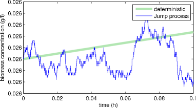
Refer to caption
Refer to caption
Figure 3: Simulation of the pure jump process with the Gillespie Algorithm 1 for K1,4=106subscript𝐾14superscript106K_{1,4}=10^{6} and K2,3,5=108subscript𝐾235superscript108K_{2,3,5}=10^{8} and 1237928 events (blue: a realization of the jump process (Xt)0t0.1subscriptsubscript𝑋𝑡0𝑡0.1(X_{t})_{0\leq t\leq 0.1}, green: the ODE (x(t))0t0.1subscript𝑥𝑡0𝑡0.1(x(t))_{0\leq t\leq 0.1}) — the substrate dynamics (RIGHT) presents many small size jumps, the biomass dynamics (LEFT) less jumps but with higher amplitude. The corresponding phase-portrait is plotted in Figure 4 (LEFT).
Refer to caption
Refer to caption
Figure 4: LEFT : Simulation of the pure jump process with the Gillespie Algorithm 1 for K1,4=106subscript𝐾14superscript106K_{1,4}=10^{6} and K2,3,5=108subscript𝐾235superscript108K_{2,3,5}=10^{8} and 1237928 events (blue: a realization of the jump process (Xt)0t0.1subscriptsubscript𝑋𝑡0𝑡0.1(X_{t})_{0\leq t\leq 0.1}, green: the ODE (x(t))0t0.1subscript𝑥𝑡0𝑡0.1(x(t))_{0\leq t\leq 0.1}) — the substrate dynamics presents many small size jumps, the biomass dynamics less jumps but with higher amplitude — the final time of simulation is 0.10.10.1 (h). RIGHT: same simulation with the Poisson approximation (X~tn)0tn0.1subscriptsubscript~𝑋subscript𝑡𝑛0subscript𝑡𝑛0.1(\tilde{X}_{t_{n}})_{0\leq t_{n}\leq 0.1} (tau-leap) with 3456 events for ε=106𝜀superscript106\varepsilon=10^{-6} (the time step is similar-to-or-equals\simeq 1.89×1051.89superscript1051.89\times 10^{-5}).
Refer to caption
Refer to caption
Figure 5: LEFT : Simulation of the Poisson approximation with the τ𝜏\tau-leap Algorithm 1 for K1,4=106subscript𝐾14superscript106K_{1,4}=10^{6} and K2,3,5=108subscript𝐾235superscript108K_{2,3,5}=10^{8} and 3004 events (blue: a realization of the jump process (X~tn)0tn100subscriptsubscript~𝑋subscript𝑡𝑛0subscript𝑡𝑛100(\tilde{X}_{t_{n}})_{0\leq t_{n}\leq 100}, green: the ODE (x(t))0t100subscript𝑥𝑡0𝑡100(x(t))_{0\leq t\leq 100}), ε=103𝜀superscript103\varepsilon=10^{-3}, ΔtΔ𝑡\Delta t between 0.0280.0280.028 and 0.03440.03440.0344. RIGHT: same simulation with the normal approximation (ξ~tn)0tn100subscriptsubscript~𝜉subscript𝑡𝑛0subscript𝑡𝑛100(\tilde{\xi}_{t_{n}})_{0\leq t_{n}\leq 100} (diffusion approximation) with 200020002000 time steps with Δt=0.05Δ𝑡0.05\Delta t=0.05.

5.2 Law of the concentrations at a given time t𝑡t

In Figure 6, we propose a Monte Carlo simulation to approximate the marginal densities of the biomass concentration Btsubscript𝐵𝑡B_{t} and of the substrate concentration Stsubscript𝑆𝑡S_{t} at a given time t𝑡t. We consider the set of parameters of Table 4 (set 1) for the Monod case in the “standard” scales K1,4=105subscript𝐾14superscript105K_{1,4}=10^{5} and K2,3,5=107subscript𝐾235superscript107K_{2,3,5}=10^{7}.

We compute (St(j),Bt(j))superscriptsubscript𝑆𝑡𝑗superscriptsubscript𝐵𝑡𝑗(S_{t}^{(j)},B_{t}^{(j)}) for t=3𝑡3t=3 (h) for j=120000𝑗120000j=1\cdots 20000 independent Monte Carlo trials of the pure jump process (with the Gillespie method), with the Poisson approximation (tau-leap method) and with the normal approximation. For the tau-leap method we choose a constant time step. For “Poisson 1” and “Normal 1” we use a step of 0.050.050.05, for “Poisson 2” and “Normal 2” we use a step of 0.50.50.5. For each test, we compute the approximate density of Stsubscript𝑆𝑡S_{t} and Btsubscript𝐵𝑡B_{t} from the sample with a kernel method. Hence we compare 5 probability density functions for each component Stsubscript𝑆𝑡S_{t} and Btsubscript𝐵𝑡B_{t}. We also compute the empirical mean and standard deviation associated with the sample obtained from the pure jump process and we plot the associated normal density.

Initial conditions are B0=0.026subscript𝐵00.026B_{0}=0.026 and S0=0.26subscript𝑆00.26S_{0}=0.26, corresponding to the case of Figure 5, which is quite far from the equilibrium state.

The conclusions are:

  • The two approximations (Poisson and normal) are very close to the exact simulation of the pure jump process; the approximation with a larger step 0.50.50.5 is slightly different.

  • The computation times222CPU time on a 2.13GHz Intel Core 2 Duo with a RAM of 2 GB. are:

    • for the exact simulation of the pure jump process: 5 h 45 min 32.6 s;

    • for the Poisson approximation: 33.2 s (with the time step 0.05) and 4.6 s (with the time step 0.5);

    • for the normal approximation: 0.7 s (with the time step 0.05) and 0.1 s (with the time step 0.5).

    In the present situation, where the parameters Kisubscript𝐾𝑖K_{i} are rather high, and for non-small concentration of the biomass and the substrate, the exact simulation of the pure jump process (Gillespie method) should be avoided.

  • The resulting empirical densities are very close to normal densities and the solution of the ODE coincide with the mean of these normal densities.

A second test is proposed in the case of the Haldane growth function (Set 2 of Table 5): see Figure 7. The conclusions are the same as for the Monod case.
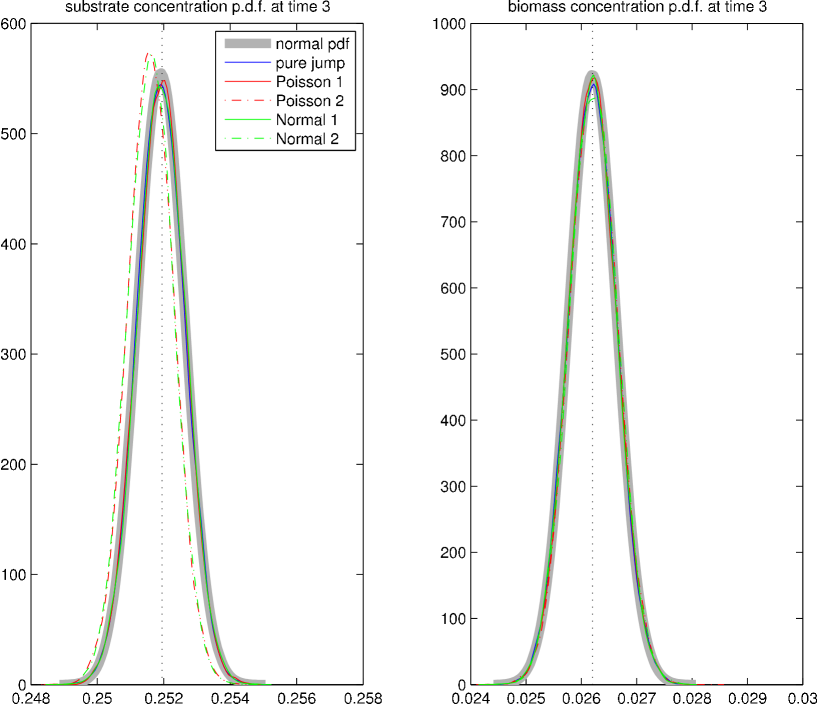
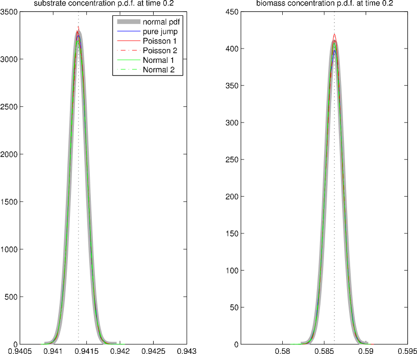
Refer to caption
Figure 6: Empirical densities for the substrate and the biomass concentrations at time t=3𝑡3t=3 obtained with the exact simulation of the pure jump process (St,Bt)subscript𝑆𝑡subscript𝐵𝑡(S_{t},B_{t}) with the Gillespie method (blue line), with the Poisson approximation (S~t,B~t)subscript~𝑆𝑡subscript~𝐵𝑡(\tilde{S}_{t},\tilde{B}_{t}) with constant time step (red solid line for a step 0.05, red dash line for a step 0.5), with the normal approximation (σ~t,β~t)subscript~𝜎𝑡subscript~𝛽𝑡(\tilde{\sigma}_{t},\tilde{\beta}_{t}) with constant time step (green solid line for a step 0.05, green dash line for a step 0.5). The corresponding CPU time are respectively: 5 h 45 min 32.6 s, 33.2 s, 4.6 s, 0.7 s, 0.1 s. The simulation parameters are the Set 1 of Table 4 (Monod growth function) with “standard” scales K1,4=105subscript𝐾14superscript105K_{1,4}=10^{5} and K2,3,5=107subscript𝐾235superscript107K_{2,3,5}=10^{7}. We compute the substrate and the biomass concentrations at t=3𝑡3t=3 (h) and for j=120000𝑗120000j=1\cdots 20000 independent Monte Carlo trials. The empirical densities are obtained with a kernel approximation procedure. We also compute the empirical mean and standard deviation from the sample of the pure jump process and plot with a thick grey line the corresponding normal densities: the match is very good. The vertical doted line the value of the substrate and biomass concentration at time t=3𝑡3t=3 given by the ODE; again it matches the mean of all the empirical densities (except the ones corresponding to the time step 0.5).
Refer to caption
Figure 7: Empirical densities for the substrate and the biomass concentrations Stsubscript𝑆𝑡S_{t} and Btsubscript𝐵𝑡B_{t} at time t=0.2𝑡0.2t=0.2 obtained with the exact simulation of the pure jump process (St,Bt)subscript𝑆𝑡subscript𝐵𝑡(S_{t},B_{t}) with the Gillespie method (blue line), with the Poisson approximation (S~t,B~t)subscript~𝑆𝑡subscript~𝐵𝑡(\tilde{S}_{t},\tilde{B}_{t}) with constant time step (red solid line for a step 0.005, red dash line for a step 0.01), with the normal approximation (σ~t,β~t)subscript~𝜎𝑡subscript~𝛽𝑡(\tilde{\sigma}_{t},\tilde{\beta}_{t}) with constant time step (green solid line for a step 0.005, green dash line for a step 0.01). The corresponding CPU time are respectively: 3 h 54 min 16.9 s, 13.5 s, 6.7 s, 0.1 s, 0.1 s. The simulation parameters are the Set 2 of Table 5 (Haldane growth function) with “standard” scales K1,4=105subscript𝐾14superscript105K_{1,4}=10^{5} and K2,3,5=107subscript𝐾235superscript107K_{2,3,5}=10^{7}. We compute the substrate and the biomass concentrations at t=0.2𝑡0.2t=0.2 (h) and for j=120000𝑗120000j=1\cdots 20000 independent Monte Carlo trials. The empirical densities are obtained with a kernel approximation procedure. We also compute the empirical mean and standard deviation from the sample of the pure jump process and plot with a thick grey line the corresponding normal densities: the match is very good. The vertical doted line the value of the substrate and biomass concentration at time t=0.2𝑡0.2t=0.2 given by the ODE; again it matches with the mean of all the empirical densities. The initial condition (S0,B0)subscript𝑆0subscript𝐵0(S_{0},B_{0}) is the stable equilibrium solution of the ODE (1) that does not correspond to the washout: hence these empirical densities could be considered as good approximations of the limit distribution of the stochastic chemostat.
Haldane model
set 1 set 2
k𝑘k 0.10.10.1 0.10.10.1 stoichiometric constant
μmaxsubscript𝜇max\mu_{\textrm{\tiny max}} 222 888 maximal growth rate (h1superscript1h^{-1})
D𝐷D 0.40.40.4 0.40.40.4 dilution rate (h1superscript1h^{-1})
sinsuperscript𝑠ins^{\textrm{\tiny in}} 111 111 input concentration (g/l𝑔𝑙g/l)
kssubscript𝑘sk_{\textrm{\tiny s}} 444 171717 half saturation constant (g/l𝑔𝑙g/l)
kisubscript𝑘𝑖k_{i} 111 111 saturation parameter )
[Uncaptioned image] [Uncaptioned image]
set 1 set 2
Table 5: Sets of simulation parameters and the corresponding Haldane growth rate functions sμ(s)𝑠𝜇𝑠s\to\mu(s). The horizontal doted line is the maximum capacity μmaxsubscript𝜇max\mu_{\textrm{\tiny max}} and the vertical doted line is the asymptotic substrate concentration of the ODE corresponding to the non-washout case.

5.3 About the scales parameters

As we have seen, for large populations, the diffusion approximation ξ~tn=(β~tn,σ~tn)subscript~𝜉subscript𝑡𝑛subscript~𝛽subscript𝑡𝑛subscript~𝜎subscript𝑡𝑛\tilde{\xi}_{t_{n}}=(\tilde{\beta}_{t_{n}},\tilde{\sigma}_{t_{n}}) given by (25) is very close to the reference pure jump model Xt=(Bt,St)subscript𝑋𝑡subscript𝐵𝑡subscript𝑆𝑡X_{t}=(B_{t},S_{t}). So we now propose simulations of the diffusion approximation in the case of a Monod specific growth rate according to the scales scenarios of Table 3

  • Case 1 (“standard”): see Figures 8 and 12.

  • Case 2 (“unstirred inflowoutflows”): see Figures 9 and 13.

  • Case 3 (“fluid substrate”): see Figures 10 and 14.

  • Case 4 (“biological only”): see Figures 11 and 15.

Figures 8 to 11 represent a simulation of a single trajectory in the 3 levels of scale: cases m,1𝑚1m,1 to m,3𝑚3m,3 (for m=14𝑚14m=1\cdots 4). Figures 12 to 15 represent the result of 10000 Monte Carlo trials in the 3 levels of scale: cases m,1𝑚1m,1 and m,2𝑚2m,2 (for m=14𝑚14m=1\cdots 4). We represent the mean trajectory and the empirical law of ξ~Tsubscript~𝜉𝑇\tilde{\xi}_{T} at final time T𝑇T.

We can conclude that, at this level of population and scale:

  • The stochasticity is negligible only in the Case 4 (“biological only”) and at the highest scale level (cases m,3𝑚3m,3).

  • The ODE solution x(t)𝑥𝑡x(t) matches the (empirical) mean of the stochastic process at these scales (as the stochastic process is solution of a nonlinear equation, there is no reason for the mean of the stochastic process to coincide with the solution of the deterministic equations).

Equivalent results have been obtained for the Haldane case.
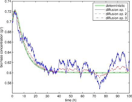
Refer to caption
Refer to caption
Refer to caption
Figure 8: Diffusion approximation, Case 1, Table 3 (“standard case”) / Simulation of (25) with Monod specific growth rate (2) with the parameters of Table 4 — Time evolution of the biomass concentration (top left), time evolution of the substrate concentration (top right), phase portrait biomass/substrate concentrations (bottom) according to 4 cases: case 0, case 1.1, case 1.2, case 1.3 (see Table 3). Cases 0 (deterministic) and 1.3 are identical.
Refer to caption
Refer to caption
Refer to caption
Figure 9: Diffusion approximation, Case 2, Table 3 (“unstirred inflow and outflows”) / Simulation of (25) with Monod specific growth rate (2) with the parameters of Table 4 — Time evolution of the biomass concentration (top left), time evolution of the substrate concentration (top right), phase portrait biomass/substrate concentrations (bottom) according to 4 cases: case 0, case 2.1, case 2.2, case 2.3 (see Table 3). Cases 0 (deterministic) and 2.3 are identical.
Refer to caption
Refer to caption
Refer to caption
Figure 10: Case 3, Table 3 (“substrate fluid limit case”) / Simulation of (25) with Monod specific growth rate (2) with the parameters of Table 4 — Time evolution of the biomass concentration (top left), time evolution of the substrate concentration (top right), phase portrait biomass/substrate concentrations (bottom) according to 4 cases: case 0, case 3.1, case 3.2, case 3.3 (see Table 3). Cases 0 (deterministic) and 3.3 are identical.
Refer to caption
Refer to caption
Refer to caption
Figure 11: Case 4, Table 3 (“biological case”) / Simulation of (25) with Monod specific growth rate (2) with the parameters of Table 4 — Time evolution of the biomass concentration (top left), time evolution of the substrate concentration (top right), phase portrait biomass/substrate concentrations (bottom) according to 4 cases: case 0, case 4.1, case 4.2, case 4.3 (see Table 3). Cases 0 (deterministic) and 4.3 are identical.
Refer to caption
Refer to caption
Figure 12: Cases 1.1 and 1.2 Table 3 / Sampling 10000 Monte Carlo trials of the law of (β~tn,σ~tn)subscript~𝛽subscript𝑡𝑛subscript~𝜎subscript𝑡𝑛(\tilde{\beta}_{t_{n}},\tilde{\sigma}_{t_{n}}) for tn=100subscript𝑡𝑛100t_{n}=100 — The deterministic solution and the mean of the sampled trajectories coincide — The final law is represented by the sample and by the contour plot of the corresponding kernel approximation of the p.d.f.
Refer to caption
Refer to caption
Figure 13: Cases 2.1 and 2.2 Table 3 / Sampling 10000 Monte Carlo trials of the law of (β~tn,σ~tn)subscript~𝛽subscript𝑡𝑛subscript~𝜎subscript𝑡𝑛(\tilde{\beta}_{t_{n}},\tilde{\sigma}_{t_{n}}) for tn=100subscript𝑡𝑛100t_{n}=100 — The deterministic solution and the mean of the sampled trajectories coincide — The final law is represented by the sample and by the contour plot of the corresponding kernel approximation of the p.d.f.
Refer to caption
Refer to caption
Figure 14: Cases 3.1 and 3.2 Table 3 / Sampling 10000 Monte Carlo trials of the law of (β~tn,σ~tn)subscript~𝛽subscript𝑡𝑛subscript~𝜎subscript𝑡𝑛(\tilde{\beta}_{t_{n}},\tilde{\sigma}_{t_{n}}) for tn=100subscript𝑡𝑛100t_{n}=100 — The deterministic solution and the mean of the sampled trajectories coincide — The final law is represented by the sample and by the contour plot of the corresponding kernel approximation of the p.d.f.
Refer to caption
Refer to caption
Figure 15: Cases 4.1 and 4.2 Table 3 / Sampling 10000 Monte Carlo trials of the law of (β~tn,σ~tn)subscript~𝛽subscript𝑡𝑛subscript~𝜎subscript𝑡𝑛(\tilde{\beta}_{t_{n}},\tilde{\sigma}_{t_{n}}) for tn=100subscript𝑡𝑛100t_{n}=100 — The deterministic solution and the mean of the sampled trajectories coincide.

5.4 Comparison with the Imhof-Walcher model [15]

We compare the processes ξt=(βt,σt)subscript𝜉𝑡superscriptsubscript𝛽𝑡subscript𝜎𝑡\xi_{t}=(\beta_{t},\sigma_{t})^{*} given by the diffusion approximation model (17) with the one given by the ad hoc model (21). The parameter are: K=1𝐾1K=1, μmax=1subscript𝜇max1\mu_{\textrm{\tiny max}}=1, D=0.5𝐷0.5D=0.5, Sin=8superscript𝑆in8S^{\textrm{\tiny in}}=8, ks=0.5subscript𝑘s0.5k_{\textrm{\tiny s}}=0.5, final time T=20𝑇20T=20, Δt=0.02Δ𝑡0.02\Delta t=0.02, 20000 Monte Carlo trials; Ki=105subscript𝐾𝑖superscript105K_{i}=10^{5} for (17) and cb=cs=0.02superscript𝑐bsuperscript𝑐s0.02c^{\textrm{\tiny b}}=c^{\textrm{\tiny s}}=0.02 for (21). The parameters are chosen so that the biomass concentration evolves from 0.5 to about 7.5, and the substrate concentration from 5 to about 0.5. Also the limit distribution is lesser than 1 in the substrate and greater than 1 in the biomass. Indeed one of the main difference between (17) and (21) is than for state values less than 1 (resp. more greater than 1) the noise variance for the first model is greater (resp. lesser) than the noise variance for the second model.

This example illustrates clearly that the two models differ substantially.
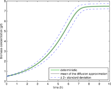
Refer to caption
Refer to caption
Refer to caption
Refer to caption
Refer to caption
Refer to caption
Figure 16: Comparison of the processes ξt=(βt,σt)subscript𝜉𝑡superscriptsubscript𝛽𝑡subscript𝜎𝑡\xi_{t}=(\beta_{t},\sigma_{t})^{*} given by the diffusion approximation model (17) and by the ad hoc model (21). Evolution of the biomass concentration (top) and substrate concentration (center) during time; final joint density approximation of concentration (bottom). The two models differ substantially: compared to the diffusion approximation, the ad hoc model overestimates (resp underestimates) the noise variance for concentration greater (resp. lesser) than 1.

6 Discussion

We started from a reference pure jump model Xtsubscript𝑋𝑡X_{t}, described by rates/jumps structure of Table 1 or as a solution of the stochastic differential equation (10). The martingale decomposition (41) clearly describes that the dynamics of Xtsubscript𝑋𝑡X_{t} is the combination of the classical deterministic dynamics of the chemostat (1) plus martingale terms with coefficients 1/Ki1subscript𝐾𝑖1/\sqrt{K_{i}} and with explicitly known quadratic variations, see (42). These quadratic variation terms allow us to assess the difference between the stochastic model and the deterministic one.

We presented the explicit Monte Carlo simulation procedure, called Gillespie method, for the process Xtsubscript𝑋𝑡X_{t}. In standard cases, that is for high population levels (i.e. Kisubscript𝐾𝑖K_{i} large), this procedure is not feasible as it requires us to simulate too many events. In this case, we presented the Poisson approximation (25b) and the normal approximation (25), both in discrete-time. These approximations are valid only for large populations, i.e. about the axes, it is necessary to return to the pure jump process representation. In the application discussed here, the Poisson approximation is of little interest: it is more time-consuming than the diffusion approximation and valid only on a very limited scale range between the pure jump model and the normal approximation model.

In contrast with previous stochastic chemostat models [26, 7, 15] where the stochasticity was introduced according to an ad hoc approach, in the present work we propose a family of models where the structure of the noise emerges from the very dynamics and where the scale parameters can be tuned according to the problem under interest. In particular it allows us to propose hybrid models where the cell population dynamics features stochasticity as the substrate is in fluid dynamics (ODE), corresponding to the Case 3 of Table 3. This kind of model has already been proposed in [11] in a three trophic levels case where the stochasticity appears only in the top level trophic as a stochastic logistic model and with fluid limit dynamics for the two other levels; it also has been proposed in [3] with a pure jump process for the biomass dynamics and a fluid limit for the substrate. This approach can also be related to coupled slow/fast reactions in stochastic chemical kinetics [13, 2].

The approach proposed here can be applied to any model of population dynamics especially in cases of difference of scale between the different dynamics (e.g. cell/substrate). The dynamics of interacting populations cannot be modeled by a single model but rather by a family of models whose domain of validity depends on the scale at which the dynamics are considered. For example the normal approximation model represented as stochastic differential equations (17) or the ODE model (1) are valid in high population levels, hence using such models to infer extinction characteristics like extinction time and extinction probabilities is not valid. This was already noticed by [22] and [27].

In most standard population scales of the chemostat the ODE model is justified. Also, the ODE framework proposes analysis, control and optimization tools that are more accessible than the one of the SDE context. Though, as seen, the stochasticity cannot be neglected in many situations. This stochasticity could be of small intensity in the present single species/single substrate situation but could deeply perturb multiple species/multiple substrates situations. The SDE model could be simulated at a small extra computational cost and offers a more realistic prediction tool. Indeed, as it can account for the variability of the experiments, the simulation of the SDE offers the possibility to explore in depth the potentialities of the dynamical systems.

The SDE model is also more adapted for the confrontation to the data as it allows us to build a statistical model and the associated likelihood function. One of the next important steps, that we will investigate in coming work, will be to propose an adapted statistical procedure to estimate the scale parameters Kisubscript𝐾𝑖K_{i}, and in a second step to estimate the parameters (D𝐷D, sinsuperscript𝑠ins^{\textrm{\tiny in}}…). In the future we will also investigate the long-term behavior of these models as well as their optimal command.

Acknowledgements

The work was partially supported by the French National Research Agency (ANR) within the SYSCOMM project DISCO ANR-09-SYSC-003.

Appendices

Appendix A Representation of the process Xtsubscript𝑋𝑡X_{t}

Infinitesimal generator

We consider the Markov process Xtsubscript𝑋𝑡X_{t} with infinitesimal generator:

𝒜ϕ(x)𝒜italic-ϕ𝑥\displaystyle{\mathcal{A}}\phi(x) =i=15λi(x)[ϕ(x+νi(x))ϕ(x)]absentsuperscriptsubscript𝑖15subscript𝜆𝑖𝑥delimited-[]italic-ϕ𝑥subscript𝜈𝑖𝑥italic-ϕ𝑥\displaystyle=\sum_{i=1}^{5}\lambda_{i}(x)\,[\phi(x+\nu_{i}(x))-\phi(x)] (26)

for all ϕ:+2:italic-ϕmaps-tosubscriptsuperscript2\phi:\mathbb{R}^{2}_{+}\mapsto\mathbb{R} continuous with compact support [6, Th. 8-3.1]. The infinitesimal generator can also be understood in the following way:

(Xt+Δt=x+y|Xt=x){λi(x)Δt+o(Δt),if y=νi(x) for i=15,1i=15λi(x)Δt+o(Δt),if y=0,o(Δt),otherwise.similar-to-or-equalssubscript𝑋𝑡Δ𝑡𝑥conditional𝑦subscript𝑋𝑡𝑥casessubscript𝜆𝑖𝑥Δ𝑡𝑜Δ𝑡if 𝑦subscript𝜈𝑖𝑥 for 𝑖151superscriptsubscript𝑖15subscript𝜆𝑖𝑥Δ𝑡𝑜Δ𝑡if 𝑦0𝑜Δ𝑡otherwise\displaystyle\mathbb{P}(X_{t+\Delta t}=x+y|X_{t}=x)\simeq\left\{\begin{array}[]{ll}\lambda_{i}(x)\,\Delta t+o(\Delta t)\,,&\textrm{if }y=\nu_{i}(x)\textrm{ for }i=1\cdots 5,\\ 1-\sum_{i=1}^{5}\lambda_{i}(x)\,\Delta t+o(\Delta t)\,,&\textrm{if }y=0,\\ o(\Delta t)\,,&\textrm{otherwise}.\end{array}\right.

or as

𝒜ϕ(x)=limt0𝔼ϕ(Xtx)ϕ(x)t𝒜italic-ϕ𝑥subscript𝑡0𝔼italic-ϕsubscriptsuperscript𝑋𝑥𝑡italic-ϕ𝑥𝑡{\mathcal{A}}\phi(x)=\lim_{t\to 0}\frac{\mathbb{E}\phi(X^{x}_{t})-\phi(x)}{t}

where Xtxsubscriptsuperscript𝑋𝑥𝑡X^{x}_{t} is the process Xtsubscript𝑋𝑡X_{t} starting from x𝑥x. It can be rewritten as:

𝒜ϕ(x)𝒜italic-ϕ𝑥\displaystyle{\mathcal{A}}\phi(x) =λ(x)+2[ϕ(y)ϕ(x)]ρ(x,dy)absent𝜆𝑥subscriptsubscriptsuperscript2delimited-[]italic-ϕ𝑦italic-ϕ𝑥𝜌𝑥d𝑦\displaystyle=\lambda(x)\,\int_{\mathbb{R}^{2}_{+}}[\phi(y)-\phi(x)]\,\rho(x,{{\textrm{d}}}y)

with

λ(x)𝜆𝑥\displaystyle\lambda(x) =defi=15λi(x),superscriptdefabsentsuperscriptsubscript𝑖15subscript𝜆𝑖𝑥\displaystyle\stackrel{{\scriptstyle{\textrm{\rm\tiny def}}}}{{=}}\sum_{i=1}^{5}\lambda_{i}(x)\,, (27)
ρ(x,dy)𝜌𝑥d𝑦\displaystyle\rho(x,{{\textrm{d}}}y) =defi=15λ¯i(x)δx+νi(x)(dy)superscriptdefabsentsuperscriptsubscript𝑖15subscript¯𝜆𝑖𝑥subscript𝛿𝑥subscript𝜈𝑖𝑥d𝑦\displaystyle\stackrel{{\scriptstyle{\textrm{\rm\tiny def}}}}{{=}}\sum_{i=1}^{5}\bar{\lambda}_{i}(x)\,\delta_{x+\nu_{i}(x)}({{\textrm{d}}}y) with λ¯i(x)=defλi(x)i=15λi(x)superscriptdefwith subscript¯𝜆𝑖𝑥subscript𝜆𝑖𝑥superscriptsubscriptsuperscript𝑖15subscript𝜆superscript𝑖𝑥\displaystyle\textrm{with }\bar{\lambda}_{i}(x)\stackrel{{\scriptstyle{\textrm{\rm\tiny def}}}}{{=}}\frac{\lambda_{i}(x)}{\sum_{i^{\prime}=1}^{5}\lambda_{i^{\prime}}(x)} (28)

We define the jump times: τ0=0subscript𝜏00\tau_{0}=0 and

τn=definf{t>τn1;XtXτn1}superscriptdefsubscript𝜏𝑛infimumformulae-sequence𝑡subscript𝜏𝑛1subscript𝑋𝑡subscript𝑋subscript𝜏𝑛1\tau_{n}\stackrel{{\scriptstyle{\textrm{\rm\tiny def}}}}{{=}}\inf\big{\{}t>\tau_{n-1}\,;\,X_{t}\neq X_{\tau_{n-1}}\big{\}}

and the embedded jump chain

Yn=defXτn.superscriptdefsubscript𝑌𝑛subscript𝑋subscript𝜏𝑛Y_{n}\stackrel{{\scriptstyle{\textrm{\rm\tiny def}}}}{{=}}X_{\tau_{n}}\,.

It is well know that (iYnsubscript𝑌𝑛Y_{n} is a Markov chain on +2subscriptsuperscript2\mathbb{R}^{2}_{+} with transition probability ρ(x,dy)𝜌𝑥d𝑦\rho(x,{{\textrm{d}}}y); (ii) for all n1𝑛1n\geq 1, conditionally on Y0,,Yn1subscript𝑌0subscript𝑌𝑛1Y_{0},\dots,Y_{n-1}, the holding times τ1τ0,,τnτn1subscript𝜏1subscript𝜏0subscript𝜏𝑛subscript𝜏𝑛1\tau_{1}-\tau_{0},\dots,\tau_{n}-\tau_{n-1} are independent and exponentially distributed of intensity parameters λ(Y0),,λ(Yn1)𝜆subscript𝑌0𝜆subscript𝑌𝑛1\lambda(Y_{0}),\dots,\lambda(Y_{n-1}), see [21]. These properties are at are the basis of the Gillespie simulation algorithm (see Algorithm 1).

Non-explosion and existence of moments

To study the non-explosion and existence of moments, we define the mean jump size function:

mK(x)=def+2(yx)ρ(x,dy)=i=15νi(x)λ¯i(x).superscriptdefsubscript𝑚𝐾𝑥subscriptsubscriptsuperscript2𝑦𝑥𝜌𝑥d𝑦superscriptsubscript𝑖15subscript𝜈𝑖𝑥subscript¯𝜆𝑖𝑥\displaystyle m_{K}(x)\stackrel{{\scriptstyle{\textrm{\rm\tiny def}}}}{{=}}\int_{\mathbb{R}^{2}_{+}}(y-x)\,\rho(x,{{\textrm{d}}}y)=\sum_{i=1}^{5}\nu_{i}(x)\,\bar{\lambda}_{i}(x)\,. (29)

and, for p1𝑝1p\geq 1

|mK|p(x)=def+2|yx|pρ(x,dy)=i=15|νi(x)|pλ¯i(x).superscriptdefsubscriptsubscript𝑚𝐾𝑝𝑥subscriptsubscriptsuperscript2superscript𝑦𝑥𝑝𝜌𝑥d𝑦superscriptsubscript𝑖15superscriptsubscript𝜈𝑖𝑥𝑝subscript¯𝜆𝑖𝑥\displaystyle|m_{K}|_{p}(x)\stackrel{{\scriptstyle{\textrm{\rm\tiny def}}}}{{=}}\int_{\mathbb{R}^{2}_{+}}|y-x|^{p}\,\rho(x,{{\textrm{d}}}y)=\sum_{i=1}^{5}|\nu_{i}(x)|^{p}\,\bar{\lambda}_{i}(x)\,. (30)

Note that from (14):

fK(x)=λ(x)mK(x)subscript𝑓𝐾𝑥𝜆𝑥subscript𝑚𝐾𝑥\displaystyle f_{K}(x)=\lambda(x)\,m_{K}(x) (31)

and if we replace νi(x)subscript𝜈𝑖𝑥\nu_{i}(x) by νisubscript𝜈𝑖\nu_{i} in (31) we get:

i=15νiλi(x)=(μ(s)bDbkμ(s)b+DsinDs)=f(x)superscriptsubscript𝑖15subscript𝜈𝑖subscript𝜆𝑖𝑥matrix𝜇𝑠𝑏𝐷𝑏𝑘𝜇𝑠𝑏𝐷superscript𝑠in𝐷𝑠𝑓𝑥\displaystyle\sum_{i=1}^{5}\nu_{i}\,\lambda_{i}(x)=\begin{pmatrix}\mu(s)\,b-D\,b\\ -k\,\mu(s)\,b+D\,s^{\textrm{\tiny in}}-D\,s\end{pmatrix}=f(x)

where f(x)𝑓𝑥f(x) is the right-hand-side function of the ODE (1).

fK(x)subscript𝑓𝐾𝑥f_{K}(x) is the instantaneous mean of the process Xtsubscript𝑋𝑡X_{t}, more precisely we will show in Proposition A.3, that 𝔼(Xt+Δt|Xt=x)fK(x)Δtsimilar-to-or-equals𝔼conditionalsubscript𝑋𝑡Δ𝑡subscript𝑋𝑡𝑥subscript𝑓𝐾𝑥Δ𝑡\mathbb{E}(X_{t+\Delta t}|X_{t}=x)\simeq f_{K}(x)\,\Delta t. As proved in the next lemma fK(x)subscript𝑓𝐾𝑥f_{K}(x) is essentially f(x)𝑓𝑥f(x), so locally in time the mean of the process Xtsubscript𝑋𝑡X_{t} behaves like x(t)𝑥𝑡x(t).

Lemma A.1

Consider νi(x)subscript𝜈𝑖𝑥\nu_{i}(x) defined in Table 1, νisubscript𝜈𝑖\nu_{i} defined by (9) and fK(x)subscript𝑓𝐾𝑥f_{K}(x) defined by (14). First |νi(x)||νi|subscript𝜈𝑖𝑥subscript𝜈𝑖|\nu_{i}(x)|\leq|\nu_{i}|. Then let

K=def{x=(bs)+2;b1K4 or s1K2 or s1K5}.{\mathcal{R}}_{K}\stackrel{{\scriptstyle{\textrm{\rm\tiny def}}}}{{=}}\Big{\{}x=\left(\begin{smallmatrix}b\\ s\end{smallmatrix}\right)\in\mathbb{R}^{2}_{+}\,;\,\textstyle b\leq\frac{1}{K_{4}}\textrm{ or }s\leq\frac{1}{K_{2}}\textrm{ or }s\leq\frac{1}{K_{5}}\Big{\}}\,.

For xK𝑥subscript𝐾x\not\in{\mathcal{R}}_{K}, νi(x)=νisubscript𝜈𝑖𝑥subscript𝜈𝑖\nu_{i}(x)=\nu_{i}, mK(x)=m(x)subscript𝑚𝐾𝑥𝑚𝑥m_{K}(x)=m(x), fK(x)=f(x)subscript𝑓𝐾𝑥𝑓𝑥f_{K}(x)=f(x). For all x+2𝑥subscriptsuperscript2x\in\mathbb{R}^{2}_{+}:

|νi(x)νi|subscript𝜈𝑖𝑥subscript𝜈𝑖\displaystyle|\nu_{i}(x)-\nu_{i}| 1minj=15Kj,i=1,,5,formulae-sequenceabsent1subscript𝑗15subscript𝐾𝑗𝑖15\displaystyle\leq\frac{1}{\min_{j=1\cdots 5}K_{j}}\,,\quad i=1,\dots,5\,, (32)
|mK(x)m(x)|subscript𝑚𝐾𝑥𝑚𝑥\displaystyle|m_{K}(x)-m(x)| 1minj=15Kj,absent1subscript𝑗15subscript𝐾𝑗\displaystyle\leq\frac{1}{\min_{j=1\cdots 5}K_{j}}\,, (33)
|fK(x)f(x)|subscript𝑓𝐾𝑥𝑓𝑥\displaystyle|f_{K}(x)-f(x)| (1K2s)+kμ(s)b+(1K4b)+Db+(1K5s)+Dsabsentsuperscript1subscript𝐾2𝑠𝑘𝜇𝑠𝑏superscript1subscript𝐾4𝑏𝐷𝑏superscript1subscript𝐾5𝑠𝐷𝑠\displaystyle\leq(1-K_{2}\,s)^{+}\,k\,\mu(s)\,b+(1-K_{4}\,b)^{+}\,D\,b+(1-K_{5}\,s)^{+}\,D\,s (34)

so that fK(x)f(x)subscript𝑓𝐾𝑥𝑓𝑥f_{K}(x)\to f(x) when Kisubscript𝐾𝑖K_{i}\to\infty for all i=1,,5𝑖15i=1,\dots,5 and this convergence is uniform on any compact set of (0,)2superscript02(0,\infty)^{2}.

Proof

For xK𝑥subscript𝐾x\not\in{\mathcal{R}}_{K} it is clear that νi(x)=νisubscript𝜈𝑖𝑥subscript𝜈𝑖\nu_{i}(x)=\nu_{i} so fK(x)=f(x)subscript𝑓𝐾𝑥𝑓𝑥f_{K}(x)=f(x). For all x𝑥x, we have ν1(x)ν1subscript𝜈1𝑥subscript𝜈1\nu_{1}(x)\equiv\nu_{1} and ν3(x)ν3subscript𝜈3𝑥subscript𝜈3\nu_{3}(x)\equiv\nu_{3} and:

ν2(x)ν2subscript𝜈2𝑥subscript𝜈2\displaystyle\nu_{2}(x)-\nu_{2} =1K2(0(1K2s)+),absent1subscript𝐾20superscript1subscript𝐾2𝑠\displaystyle=\textstyle\frac{1}{K_{2}}\left(\begin{smallmatrix}0\\ (1-K_{2}\,s)^{+}\end{smallmatrix}\right)\,,
ν4(x)ν4subscript𝜈4𝑥subscript𝜈4\displaystyle\nu_{4}(x)-\nu_{4} =1K4((1K4b)+0),absent1subscript𝐾4superscript1subscript𝐾4𝑏0\displaystyle=\textstyle\frac{1}{K_{4}}\left(\begin{smallmatrix}(1-K_{4}\,b)^{+}\\ 0\end{smallmatrix}\right)\,,
ν5(x)ν5subscript𝜈5𝑥subscript𝜈5\displaystyle\nu_{5}(x)-\nu_{5} =1K5(0(1K5s)+)absent1subscript𝐾50superscript1subscript𝐾5𝑠\displaystyle=\textstyle\frac{1}{K_{5}}\left(\begin{smallmatrix}0\\ (1-K_{5}\,s)^{+}\end{smallmatrix}\right)

so we get (32). The following assertions of the lemma are straightforward. \Box


Non-explosion and existence of moments are given by the following result:

Theorem A.2 (Hamza and Klebaner [12])

Suppose that λ(x)>0𝜆𝑥0\lambda(x)>0 for all x+2𝑥subscriptsuperscript2x\in\mathbb{R}^{2}_{+} and that there exist C>0𝐶0C>0 and p1𝑝1p\geq 1 such that 𝔼(|X0|p)<𝔼superscriptsubscript𝑋0𝑝\mathbb{E}(|X_{0}|^{p})<\infty and

λ(x)|fK|p(x)C(1+|x|p),x+2formulae-sequence𝜆𝑥subscriptsubscript𝑓𝐾𝑝𝑥𝐶1superscript𝑥𝑝for-all𝑥subscriptsuperscript2\displaystyle\lambda(x)\,|f_{K}|_{p}(x)\leq C\,(1+|x|^{p})\,,\quad\forall x\in\mathbb{R}^{2}_{+} (35)

then the Markov process (Xt)t0subscriptsubscript𝑋𝑡𝑡0(X_{t})_{t\geq 0} is non-explosive, that is τnsubscript𝜏𝑛\tau_{n}\to\infty a.s., and for all T>0𝑇0T>0 there exists C>0𝐶0C>0 s.t. 𝔼(|Xt|p)C𝔼superscriptsubscript𝑋𝑡𝑝𝐶\mathbb{E}(|X_{t}|^{p})\leq C for all tT𝑡𝑇t\leq T.

Indeed λ(x)=iλi(x)K3Dsin>0𝜆𝑥subscript𝑖subscript𝜆𝑖𝑥subscript𝐾3𝐷superscript𝑠in0\lambda(x)=\sum_{i}\lambda_{i}(x)\geq K_{3}\,D\,s^{\textrm{\tiny in}}>0 and

|fK|p(x)subscriptsubscript𝑓𝐾𝑝𝑥\displaystyle|f_{K}|_{p}(x) =i=15|νi(x)|pλ¯i(x)absentsuperscriptsubscript𝑖15superscriptsubscript𝜈𝑖𝑥𝑝subscript¯𝜆𝑖𝑥\displaystyle=\sum_{i=1}^{5}|\nu_{i}(x)|^{p}\,\bar{\lambda}_{i}(x)
μ(s)bK1p1+kμ(s)bK2p1+DsinK3p1+DbK4p1+DsK5p1absent𝜇𝑠𝑏superscriptsubscript𝐾1𝑝1𝑘𝜇𝑠𝑏superscriptsubscript𝐾2𝑝1𝐷superscript𝑠insuperscriptsubscript𝐾3𝑝1𝐷𝑏superscriptsubscript𝐾4𝑝1𝐷𝑠superscriptsubscript𝐾5𝑝1\displaystyle\leq\frac{\mu(s)\,b}{K_{1}^{p-1}}+\frac{k\,\mu(s)\,b}{K_{2}^{p-1}}+\frac{D\,s^{\textrm{\tiny in}}}{K_{3}^{p-1}}+\frac{D\,b}{K_{4}^{p-1}}+\frac{D\,s}{K_{5}^{p-1}}
(1K1p1+1K2p1+1K3p1+1K4p1+1K5p1)(1+|x|)absent1superscriptsubscript𝐾1𝑝11superscriptsubscript𝐾2𝑝11superscriptsubscript𝐾3𝑝11superscriptsubscript𝐾4𝑝11superscriptsubscript𝐾5𝑝11𝑥\displaystyle\leq\Big{(}\frac{1}{K_{1}^{p-1}}+\frac{1}{K_{2}^{p-1}}+\frac{1}{K_{3}^{p-1}}+\frac{1}{K_{4}^{p-1}}+\frac{1}{K_{5}^{p-1}}\Big{)}\,(1+|x|)

so that (35) is fulfilled for all p1𝑝1p\geq 1. Hence the Markov process Xtsubscript𝑋𝑡X_{t} with infinitesimal generator 𝒜𝒜{\mathcal{A}} defined by (26) is non-explosive and Xtsubscript𝑋𝑡X_{t} admits moments of all order for all t0𝑡0t\geq 0.

Representation for the process Xtsubscript𝑋𝑡X_{t}

We now give a representation for the process Xtsubscript𝑋𝑡X_{t} as a solution of a stochastic differential equation driven by random Poisson measures:

Proposition A.3

The process Xtsubscript𝑋𝑡X_{t} is defined for all t0𝑡0t\geq 0 and it is solution of the jump SDE (10) where Nisuperscript𝑁𝑖N^{i} are independent random Poisson measures with intensity measure du×dvd𝑢d𝑣{{\textrm{d}}}u\times{{\textrm{d}}}v (Lebesgue measure).

Proof

We first verify that the stochastic integral in (10) is defined. According to [14, § II-3], this integral is defined if:

𝔼0t0|νi(Xu)|missing1{vλi(Xu)}dvdu<.𝔼superscriptsubscript0𝑡superscriptsubscript0subscript𝜈𝑖subscript𝑋𝑢subscriptmissing1𝑣subscript𝜆𝑖subscript𝑋𝑢d𝑣d𝑢\mathbb{E}\int_{0}^{t}\int_{0}^{\infty}|\nu_{i}(X_{u})|\,{\mathrm{\mathbf{missing}}1}_{\{v\leq\lambda_{i}(X_{u})\}}\,{{\textrm{d}}}v\,{{\textrm{d}}}u<\infty\,.

We have

𝔼0t0|νi(Xu)|missing1{vλi(Xu)}dvdu𝔼superscriptsubscript0𝑡superscriptsubscript0subscript𝜈𝑖subscript𝑋𝑢subscriptmissing1𝑣subscript𝜆𝑖subscript𝑋𝑢d𝑣d𝑢\displaystyle\mathbb{E}\int_{0}^{t}\int_{0}^{\infty}|\nu_{i}(X_{u})|\,{\mathrm{\mathbf{missing}}1}_{\{v\leq\lambda_{i}(X_{u})\}}\,{{\textrm{d}}}v\,{{\textrm{d}}}u
1Ki𝔼0tλi(Xu)duC0t(1+𝔼|Xu|)duabsent1subscript𝐾𝑖𝔼superscriptsubscript0𝑡subscript𝜆𝑖subscript𝑋𝑢d𝑢𝐶superscriptsubscript0𝑡1𝔼subscript𝑋𝑢d𝑢\displaystyle\qquad\qquad\qquad\leq\frac{1}{K_{i}}\,\mathbb{E}\int_{0}^{t}\lambda_{i}(X_{u})\,{{\textrm{d}}}u\leq C\,\int_{0}^{t}(1+\mathbb{E}|X_{u}|)\,{{\textrm{d}}}u

which is finite according to Theorem A.2. \Box


Consider the centered random Poisson measure:

N~i(du×dv)=defNi(du×dv)du×dv.superscriptdefsuperscript~𝑁𝑖d𝑢d𝑣superscript𝑁𝑖d𝑢d𝑣d𝑢d𝑣\tilde{N}^{i}({{\textrm{d}}}u\times{{\textrm{d}}}v)\stackrel{{\scriptstyle{\textrm{\rm\tiny def}}}}{{=}}N^{i}({{\textrm{d}}}u\times{{\textrm{d}}}v)-{{\textrm{d}}}u\times{{\textrm{d}}}v\,.

According to [14, § II-3]

Mti=def0t0νi(Xu)missing1{vλi(Xu)}N~i(du×dv),i=1,,5formulae-sequencesuperscriptdefsubscriptsuperscript𝑀𝑖𝑡superscriptsubscript0𝑡superscriptsubscript0subscript𝜈𝑖subscript𝑋superscript𝑢subscriptmissing1𝑣subscript𝜆𝑖subscript𝑋superscript𝑢superscript~𝑁𝑖d𝑢d𝑣𝑖15\displaystyle M^{i}_{t}\stackrel{{\scriptstyle{\textrm{\rm\tiny def}}}}{{=}}\int_{0}^{t}\int_{0}^{\infty}\nu_{i}(X_{u^{-}})\,{\mathrm{\mathbf{missing}}1}_{\{v\leq\lambda_{i}(X_{u^{-}})\}}\,\tilde{N}^{i}({{\textrm{d}}}u\times{{\textrm{d}}}v)\,,\qquad i=1,\dots,5 (36)

are five independent square-integrable martingales with finite moments of all orders. Let:

Mt=defi=15Mti.superscriptdefsubscript𝑀𝑡superscriptsubscript𝑖15subscriptsuperscript𝑀𝑖𝑡\displaystyle M_{t}\stackrel{{\scriptstyle{\textrm{\rm\tiny def}}}}{{=}}\sum_{i=1}^{5}M^{i}_{t}\,. (37)

From (10):

Xtsubscript𝑋𝑡\displaystyle X_{t} =X0+0tfK(Xu)du+Mt.absentsubscript𝑋0superscriptsubscript0𝑡subscript𝑓𝐾subscript𝑋𝑢d𝑢subscript𝑀𝑡\displaystyle=X_{0}+\int_{0}^{t}f_{K}(X_{u})\,{{\textrm{d}}}u+M_{t}\,. (38)

We want to study the behavior of the martingales Mtisubscriptsuperscript𝑀𝑖𝑡M^{i}_{t} as the Kisubscript𝐾𝑖K_{i}\to\infty. First note that Mti=(mti0)subscriptsuperscript𝑀𝑖𝑡subscriptsuperscript𝑚𝑖𝑡0M^{i}_{t}=\left(\begin{smallmatrix}m^{i}_{t}\\ 0\end{smallmatrix}\right) for i=1,4𝑖14i=1,4 and Mti=(0mti)subscriptsuperscript𝑀𝑖𝑡0subscriptsuperscript𝑚𝑖𝑡M^{i}_{t}=\left(\begin{smallmatrix}0\\ m^{i}_{t}\end{smallmatrix}\right) for i=2,3,5𝑖235i=2,3,5 with

mt1subscriptsuperscript𝑚1𝑡\displaystyle m^{1}_{t} =def1K10t0missing1{vλ1(Xu)}N~1(du×dv),superscriptdefabsent1subscript𝐾1superscriptsubscript0𝑡superscriptsubscript0subscriptmissing1𝑣subscript𝜆1subscript𝑋superscript𝑢superscript~𝑁1d𝑢d𝑣\displaystyle\stackrel{{\scriptstyle{\textrm{\rm\tiny def}}}}{{=}}\hphantom{-}\frac{1}{K_{1}}\,\int_{0}^{t}\int_{0}^{\infty}{\mathrm{\mathbf{missing}}1}_{\{v\leq\lambda_{1}(X_{u^{-}})\}}\,\tilde{N}^{1}({{\textrm{d}}}u\times{{\textrm{d}}}v)\,, (39a)
mt2subscriptsuperscript𝑚2𝑡\displaystyle m^{2}_{t} =def1K20t0(1K2Su)missing1{vλ2(Xu)}N~2(du×dv),superscriptdefabsent1subscript𝐾2superscriptsubscript0𝑡superscriptsubscript01subscript𝐾2subscript𝑆superscript𝑢subscriptmissing1𝑣subscript𝜆2subscript𝑋superscript𝑢superscript~𝑁2d𝑢d𝑣\displaystyle\stackrel{{\scriptstyle{\textrm{\rm\tiny def}}}}{{=}}-\frac{1}{K_{2}}\,\int_{0}^{t}\int_{0}^{\infty}(1\wedge K_{2}\,S_{u^{-}})\,{\mathrm{\mathbf{missing}}1}_{\{v\leq\lambda_{2}(X_{u^{-}})\}}\,\tilde{N}^{2}({{\textrm{d}}}u\times{{\textrm{d}}}v)\,, (39b)
mt3subscriptsuperscript𝑚3𝑡\displaystyle m^{3}_{t} =def1K30t0missing1{vλ3(Xu)}N~3(du×dv),superscriptdefabsent1subscript𝐾3superscriptsubscript0𝑡superscriptsubscript0subscriptmissing1𝑣subscript𝜆3subscript𝑋superscript𝑢superscript~𝑁3d𝑢d𝑣\displaystyle\stackrel{{\scriptstyle{\textrm{\rm\tiny def}}}}{{=}}\hphantom{-}\frac{1}{K_{3}}\,\int_{0}^{t}\int_{0}^{\infty}{\mathrm{\mathbf{missing}}1}_{\{v\leq\lambda_{3}(X_{u^{-}})\}}\,\tilde{N}^{3}({{\textrm{d}}}u\times{{\textrm{d}}}v)\,, (39c)
mt4subscriptsuperscript𝑚4𝑡\displaystyle m^{4}_{t} =def1K40t0(1K4Bu)missing1{vλ4(Xu)}N~4(du×dv),superscriptdefabsent1subscript𝐾4superscriptsubscript0𝑡superscriptsubscript01subscript𝐾4subscript𝐵superscript𝑢subscriptmissing1𝑣subscript𝜆4subscript𝑋superscript𝑢superscript~𝑁4d𝑢d𝑣\displaystyle\stackrel{{\scriptstyle{\textrm{\rm\tiny def}}}}{{=}}-\frac{1}{K_{4}}\,\int_{0}^{t}\int_{0}^{\infty}(1\wedge K_{4}\,B_{u^{-}})\,{\mathrm{\mathbf{missing}}1}_{\{v\leq\lambda_{4}(X_{u^{-}})\}}\,\tilde{N}^{4}({{\textrm{d}}}u\times{{\textrm{d}}}v)\,, (39d)
mt5subscriptsuperscript𝑚5𝑡\displaystyle m^{5}_{t} =def1K50t0(1K5Su)missing1{vλ5(Xu)}N~5(du×dv).superscriptdefabsent1subscript𝐾5superscriptsubscript0𝑡superscriptsubscript01subscript𝐾5subscript𝑆superscript𝑢subscriptmissing1𝑣subscript𝜆5subscript𝑋superscript𝑢superscript~𝑁5d𝑢d𝑣\displaystyle\stackrel{{\scriptstyle{\textrm{\rm\tiny def}}}}{{=}}-\frac{1}{K_{5}}\,\int_{0}^{t}\int_{0}^{\infty}(1\wedge K_{5}\,S_{u^{-}})\,{\mathrm{\mathbf{missing}}1}_{\{v\leq\lambda_{5}(X_{u^{-}})\}}\,\tilde{N}^{5}({{\textrm{d}}}u\times{{\textrm{d}}}v)\,. (39e)

As mtisubscriptsuperscript𝑚𝑖𝑡m^{i}_{t} is of the form mti=0t0γi(u,v)N~i(du×dv)subscriptsuperscript𝑚𝑖𝑡superscriptsubscript0𝑡superscriptsubscript0superscript𝛾𝑖superscript𝑢𝑣superscript~𝑁𝑖d𝑢d𝑣m^{i}_{t}=\int_{0}^{t}\int_{0}^{\infty}\gamma^{i}(u^{-},v)\,\tilde{N}^{i}({{\textrm{d}}}u\times{{\textrm{d}}}v) then the associated predictable quadratic variation is mit=0t0[γi(u,v)]2dvdusubscriptdelimited-⟨⟩superscript𝑚𝑖𝑡superscriptsubscript0𝑡superscriptsubscript0superscriptdelimited-[]superscript𝛾𝑖𝑢𝑣2d𝑣d𝑢\langle m^{i}\rangle_{t}=\int_{0}^{t}\int_{0}^{\infty}[\gamma^{i}(u,v)]^{2}\,{{\textrm{d}}}v\,{{\textrm{d}}}u so we can easily check that

m1tsubscriptdelimited-⟨⟩superscript𝑚1𝑡\displaystyle\langle m^{1}\rangle_{t} =1K10tμ(Su)Budu,absent1subscript𝐾1superscriptsubscript0𝑡𝜇subscript𝑆𝑢subscript𝐵𝑢d𝑢\displaystyle=\frac{1}{K_{1}}\,\int_{0}^{t}\mu(S_{u})\,B_{u}\,{{\textrm{d}}}u\,,
m2tsubscriptdelimited-⟨⟩superscript𝑚2𝑡\displaystyle\langle m^{2}\rangle_{t} =1K20t(1K2Su)2kμ(Su)Budu,absent1subscript𝐾2superscriptsubscript0𝑡superscript1subscript𝐾2subscript𝑆𝑢2𝑘𝜇subscript𝑆𝑢subscript𝐵𝑢d𝑢\displaystyle=\frac{1}{K_{2}}\,\int_{0}^{t}(1\wedge K_{2}\,S_{u})^{2}\,k\,\mu(S_{u})\,B_{u}\,{{\textrm{d}}}u\,,
m3tsubscriptdelimited-⟨⟩superscript𝑚3𝑡\displaystyle\langle m^{3}\rangle_{t} =1K3Dsint,absent1subscript𝐾3𝐷superscript𝑠in𝑡\displaystyle=\frac{1}{K_{3}}\,D\,s^{\textrm{\tiny in}}\,t\,,
m4tsubscriptdelimited-⟨⟩superscript𝑚4𝑡\displaystyle\langle m^{4}\rangle_{t} =1K40t(1K4Bu)2DBudu,absent1subscript𝐾4superscriptsubscript0𝑡superscript1subscript𝐾4subscript𝐵𝑢2𝐷subscript𝐵𝑢d𝑢\displaystyle=\frac{1}{K_{4}}\,\int_{0}^{t}(1\wedge K_{4}\,B_{u})^{2}\,D\,B_{u}\,{{\textrm{d}}}u\,,
m5tsubscriptdelimited-⟨⟩superscript𝑚5𝑡\displaystyle\langle m^{5}\rangle_{t} =1K50t(1K5Su)2DSudu.absent1subscript𝐾5superscriptsubscript0𝑡superscript1subscript𝐾5subscript𝑆𝑢2𝐷subscript𝑆𝑢d𝑢\displaystyle=\frac{1}{K_{5}}\,\int_{0}^{t}(1\wedge K_{5}\,S_{u})^{2}\,D\,S_{u}\,{{\textrm{d}}}u\,.

Define

m¯ti=defKimti=Ki[0,t]×[0,)γi(u,v)N~i(du×dv).superscriptdefsubscriptsuperscript¯𝑚𝑖𝑡subscript𝐾𝑖subscriptsuperscript𝑚𝑖𝑡subscript𝐾𝑖subscript0𝑡0superscript𝛾𝑖superscript𝑢𝑣superscript~𝑁𝑖d𝑢d𝑣\displaystyle\bar{m}^{i}_{t}\stackrel{{\scriptstyle{\textrm{\rm\tiny def}}}}{{=}}\sqrt{K_{i}}\,m^{i}_{t}=\sqrt{K_{i}}\,\int_{[0,t]\times[0,\infty)}\gamma^{i}(u^{-},v)\,\tilde{N}^{i}({{\textrm{d}}}u\times{{\textrm{d}}}v)\,. (40)

So we obtained the following representation of the process Xtsubscript𝑋𝑡X_{t} that emphases the dependence on the Kisubscript𝐾𝑖K_{i}:

dBtdsubscript𝐵𝑡\displaystyle{{\textrm{d}}}B_{t} =(μ(St)Bt(1K4Bt)DBt)dt+1K1dm¯t1+1K4dm¯t4absent𝜇subscript𝑆𝑡subscript𝐵𝑡1subscript𝐾4subscript𝐵𝑡𝐷subscript𝐵𝑡d𝑡1subscript𝐾1dsubscriptsuperscript¯𝑚1𝑡1subscript𝐾4dsubscriptsuperscript¯𝑚4𝑡\displaystyle=\big{(}\mu(S_{t})\,B_{t}-(1\wedge K_{4}\,B_{t})\,D\,B_{t}\big{)}\,{{\textrm{d}}}t\textstyle+\frac{1}{\sqrt{K_{1}}}\,{{\textrm{d}}}\bar{m}^{1}_{t}+\frac{1}{\sqrt{K_{4}}}\,{{\textrm{d}}}\bar{m}^{4}_{t} (41a)
dStdsubscript𝑆𝑡\displaystyle{{\textrm{d}}}S_{t} =((1K2St)kμ(St)Bt+Dsin(1K5St)DSt)dtabsent1subscript𝐾2subscript𝑆𝑡𝑘𝜇subscript𝑆𝑡subscript𝐵𝑡𝐷superscript𝑠in1subscript𝐾5subscript𝑆𝑡𝐷subscript𝑆𝑡d𝑡\displaystyle=\big{(}-(1\wedge K_{2}\,S_{t})\,k\,\mu(S_{t})\,B_{t}+D\,s^{\textrm{\tiny in}}-(1\wedge K_{5}\,S_{t})\,D\,S_{t}\big{)}\,{{\textrm{d}}}t
+1K2dm¯t2+1K3dm¯t3+1K5dm¯t51subscript𝐾2dsubscriptsuperscript¯𝑚2𝑡1subscript𝐾3dsubscriptsuperscript¯𝑚3𝑡1subscript𝐾5dsubscriptsuperscript¯𝑚5𝑡\displaystyle\qquad\qquad\qquad\qquad\qquad\qquad\textstyle+\frac{1}{\sqrt{K_{2}}}\,{{\textrm{d}}}\bar{m}^{2}_{t}+\frac{1}{\sqrt{K_{3}}}\,{{\textrm{d}}}\bar{m}^{3}_{t}+\frac{1}{\sqrt{K_{5}}}\,{{\textrm{d}}}\bar{m}^{5}_{t} (41b)

where m¯tisubscriptsuperscript¯𝑚𝑖𝑡\bar{m}^{i}_{t} are independent square integrable martingales with the following quadratic variations:

m¯1tsubscriptdelimited-⟨⟩superscript¯𝑚1𝑡\displaystyle\langle\bar{m}^{1}\rangle_{t} =0tμ(Su)Budu,absentsuperscriptsubscript0𝑡𝜇subscript𝑆𝑢subscript𝐵𝑢d𝑢\displaystyle=\int_{0}^{t}\mu(S_{u})\,B_{u}\,{{\textrm{d}}}u\,, (42a)
m¯2tsubscriptdelimited-⟨⟩superscript¯𝑚2𝑡\displaystyle\langle\bar{m}^{2}\rangle_{t} =0t(1K2Su)2kμ(Su)Budu,absentsuperscriptsubscript0𝑡superscript1subscript𝐾2subscript𝑆𝑢2𝑘𝜇subscript𝑆𝑢subscript𝐵𝑢d𝑢\displaystyle=\int_{0}^{t}(1\wedge K_{2}\,S_{u})^{2}\,k\,\mu(S_{u})\,B_{u}\,{{\textrm{d}}}u\,, (42b)
m¯3tsubscriptdelimited-⟨⟩superscript¯𝑚3𝑡\displaystyle\langle\bar{m}^{3}\rangle_{t} =Dsint,absent𝐷superscript𝑠in𝑡\displaystyle=D\,s^{\textrm{\tiny in}}\,t\vphantom{\int_{0}^{t}}\,, (42c)
m¯4tsubscriptdelimited-⟨⟩superscript¯𝑚4𝑡\displaystyle\langle\bar{m}^{4}\rangle_{t} =0t(1K4Bu)2DBudu,absentsuperscriptsubscript0𝑡superscript1subscript𝐾4subscript𝐵𝑢2𝐷subscript𝐵𝑢d𝑢\displaystyle=\int_{0}^{t}(1\wedge K_{4}\,B_{u})^{2}\,D\,B_{u}\,{{\textrm{d}}}u\,, (42d)
m¯5tsubscriptdelimited-⟨⟩superscript¯𝑚5𝑡\displaystyle\langle\bar{m}^{5}\rangle_{t} =0t(1K5Su)2DSudu.absentsuperscriptsubscript0𝑡superscript1subscript𝐾5subscript𝑆𝑢2𝐷subscript𝑆𝑢d𝑢\displaystyle=\int_{0}^{t}(1\wedge K_{5}\,S_{u})^{2}\,D\,S_{u}\,{{\textrm{d}}}u\,. (42e)

Appendix B Existence and uniqueness for a solution of the SDE (17)

To prove that the system (17) admits a strong solution and pathwise uniqueness holds we use the results of [24, p. 134] or [5]. Let 𝒟N=[1N,N]×[K5K3sin+1N,N]subscript𝒟𝑁1𝑁𝑁subscript𝐾5subscript𝐾3superscript𝑠in1𝑁𝑁{\mathcal{D}}_{N}=[\frac{1}{N},N]\times[-\frac{K_{5}}{K_{3}}\,s^{\textrm{\tiny in}}+\frac{1}{N},N] and rewrite (17) as:

dξt=f(ξt)dt+g(ξt)dWtdsubscript𝜉𝑡𝑓subscript𝜉𝑡d𝑡𝑔subscript𝜉𝑡dsubscript𝑊𝑡\displaystyle{{\textrm{d}}}\xi_{t}=f(\xi_{t})\,{{\textrm{d}}}t+g(\xi_{t})\,{{\textrm{d}}}W_{t} (43)

where ξt=(βt,σt)subscript𝜉𝑡superscriptsubscript𝛽𝑡subscript𝜎𝑡\xi_{t}=(\beta_{t},\sigma_{t})^{*} and Wt=(Wtb,Wts)subscript𝑊𝑡superscriptsubscriptsuperscript𝑊b𝑡subscriptsuperscript𝑊s𝑡W_{t}=(W^{\textrm{\tiny b}}_{t},W^{\textrm{\tiny s}}_{t})^{*}. The coefficient g𝑔g is not Lipschitz continuous, it is globally Lipschitz on 𝒟Nsubscript𝒟𝑁{\mathcal{D}}_{N} for all N𝑁N, but we can find Lipschitz continuous coefficients fNsubscript𝑓𝑁f_{N} and gNsubscript𝑔𝑁g_{N} such that:

fN(ξ)subscript𝑓𝑁𝜉\displaystyle f_{N}(\xi) =f(ξ) for ξ𝒟N,absent𝑓𝜉 for 𝜉subscript𝒟𝑁\displaystyle=f(\xi)\textrm{ for }\xi\in{\mathcal{D}}_{N}\,, fN(ξ)subscript𝑓𝑁𝜉\displaystyle f_{N}(\xi) =0 for ξ𝒟2N,absent0 for 𝜉subscript𝒟2𝑁\displaystyle=0\textrm{ for }\xi\not\in{\mathcal{D}}_{2N}\,,
gN(ξ)subscript𝑔𝑁𝜉\displaystyle g_{N}(\xi) =g(ξ) for ξ𝒟N,absent𝑔𝜉 for 𝜉subscript𝒟𝑁\displaystyle=g(\xi)\textrm{ for }\xi\in{\mathcal{D}}_{N}\,, gN(ξ)subscript𝑔𝑁𝜉\displaystyle g_{N}(\xi) =0 for ξ𝒟2N.absent0 for 𝜉subscript𝒟2𝑁\displaystyle=0\textrm{ for }\xi\not\in{\mathcal{D}}_{2N}\,.

The the system

dξtN=fN(ξtN)dt+gN(ξtN)dWtdsuperscriptsubscript𝜉𝑡𝑁subscript𝑓𝑁superscriptsubscript𝜉𝑡𝑁d𝑡subscript𝑔𝑁superscriptsubscript𝜉𝑡𝑁dsubscript𝑊𝑡\displaystyle{{\textrm{d}}}\xi_{t}^{N}=f_{N}(\xi_{t}^{N})\,{{\textrm{d}}}t+g_{N}(\xi_{t}^{N})\,{{\textrm{d}}}W_{t}

admits a unique strong solution ξNsuperscript𝜉𝑁\xi^{N}. Let:

TN=inf{t0;ξtN𝒟N}.subscript𝑇𝑁infimumformulae-sequence𝑡0superscriptsubscript𝜉𝑡𝑁subscript𝒟𝑁T_{N}=\inf\{t\geq 0\,;\,\xi_{t}^{N}\not\in{\mathcal{D}}_{N}\}\,.

Hence if NM𝑁𝑀N\geq M then ξN=ξMsuperscript𝜉𝑁superscript𝜉𝑀\xi^{N}=\xi^{M} for all tTM𝑡subscript𝑇𝑀t\leq T_{M}, so we can define a process ξsuperscript𝜉\xi^{\infty} such that:

ξt=ξtNtTNformulae-sequencesubscriptsuperscript𝜉𝑡subscriptsuperscript𝜉𝑁𝑡for-all𝑡subscript𝑇𝑁\xi^{\infty}_{t}=\xi^{N}_{t}\quad\forall t\leq T_{N}

and will be solution of (43) up to the explosion time T=limNTNsubscript𝑇subscript𝑁subscript𝑇𝑁T_{\infty}=\lim_{N\to\infty}T_{N}. Then by stability property and by the fact that the solution cannot cross the boundary of 𝒟𝒟{\mathcal{D}} we get T=subscript𝑇T_{\infty}=\infty a.s. which proves the strong existence and pathwise uniqueness defined for all t0𝑡0t\geq 0.

References

  • [1] David F. Anderson, Arnab Ganguly, and Thomas G. Kurtz. Error analysis of tau-leap simulation methods. Submitted to the Annals of Applied Probability arXiv: math.PR/0909.4790, 2009.
  • [2] Karen Ball, Thomas G. Kurtz, Lea Popovic, and Greg Rempala. Asymptotic analysis of multiscale approximations to reaction networks. Annals of Applied Probability, 16(4):1925–1961, 2006.
  • [3] Kenny S. Crump and Wan-Shin C. O’Young. Some stochastic features of bacterial constant growth apparatus. Bulletin of Mathematical Biology, 41(1):53 – 66, 1979.
  • [4] Awa Diop. Sur la discrétisation et le comportement à petit bruit d’EDS unidimensionnelles dont les coefficients sont à dérivées singulières. PhD thesis, Université de Nice-Sophia-Antipolis, 2003.
  • [5] Richard Durrett. Stochastic Calculus: A Practical Introduction. CRC Press, 1996.
  • [6] Stewart N. Ethier and Thomas G. Kurtz. Markov Processes – Characterization and Convergence. John Wiley & Sons, 1986.
  • [7] Thomas C. Gard. Asymptotic and transient analysis of stochastic core ecosystem models. In Fourth Mississippi State Conference on Differential Equations and Computational Simulations, Electronic Journal of Differential Equations, Conference 03, pages 51–62, 1999.
  • [8] Daniel T. Gillespie. The chemical Langevin equation. The Journal of Chemical Physics, 113(1):297–306, 2000.
  • [9] Daniel T. Gillespie. Approximate accelerated stochastic simulation of chemically reacting systems. Journal of Chemical Physics, 115(4):1716–1733, 2001.
  • [10] Daniel T. Gillespie and Linda R. Petzold. Improved leap-size selection for accelerated stochastic simulation. J. Chem. Phys., 119:8229–8234, October 2003.
  • [11] Johan Grasman and Maarten De Gee. Breakdown of a chemostat exposed to stochastic noise volume. Journal of Engineering Mathematics, 53(3):291–300, 2005.
  • [12] Kais Hamza and Fima C. Klebaner. Conditions for integrability of Markov chains. Journal of Applied Probability, 32(2):541–547, 1995.
  • [13] Eric L. Haseltine and James B. Rawlings. Approximate simulation of coupled fast and slow reactions for stochastic chemical kinetics. Journal of Chemical Physics, 117(15):6959–6969, 2002.
  • [14] Nobuyuki Ikeda and Shinzo Watanabe. Stochastic Differential Equations and Diffusion Processes. North–Holland/Kodansha, Amsterdam, 1981.
  • [15] Lorens Imhof and Sebastian Walcher. Exclusion and persistence in deterministic and stochastic chemostat models. Journal of Differential Equations, 217(1):26–53, 2005.
  • [16] Marc Joannides and Irène Larramendy-Valverde. On geometry and scale of a stochastic chemostat. In Stochastic Modeling Techniques and Data Analysis International Conference (SMTDA), 2010.
  • [17] Thomas G. Kurtz. Solutions of ordinary differential equations as limits of pure jump Markov processes. Journal of Applied Probability, 7(1):49–58, 1970.
  • [18] Thomas G. Kurtz. Limit theorems for sequences of jump Markov processes approximating ordinary differential processes. Journal of Applied Probability, 8:344–356, 1971.
  • [19] Damien Lamberton and Bernard Lapeyre. Introduction to Stochastic Calculus Applied to Finance. Chapman & Hall/CRC, 1996.
  • [20] Tiejun Li. Analysis of explicit tau-leaping schemes for simulating chemically reacting systems. Multiscale Modeling & Simulation, 6(2):417–436, 2007.
  • [21] James R. Norris. Markov chains. Cambridge University Press, 1998.
  • [22] Philip Pollett. Diffusion approximations for ecological models. In Proceedings of the International Congress of Modelling and Simulation, 2001.
  • [23] Muruhan Rathinam, Linda R. Petzold, Yang Cao, and Daniel T. Gillespie. Consistency and stability of tau-leaping schemes for chemical reaction systems. Multiscale Modeling & Simulation, 3:867–895, 2005.
  • [24] L. C. G. Rogers and David Williams. Diffusions, Markov Processes, and Martingales, volume 2, Itô Calculus. Cambridge University Press, 2nd edition edition, 2000.
  • [25] Hal L. Smith and Paul E. Waltman. The Theory of the Chemostat: Dynamics of Microbial Competition. Cambridge University Press, 1995.
  • [26] G. Stephanopoulos, R. Aris, and A.G. Fredrickson. A stochastic analysis of the growth of competing microbial populations in a continuous biochemical reactor. Mathematical Biosciences, 45:99–135, 1979.
  • [27] Chris Wilcox and Hugh Possingham. Do life history traits affect the accuracy of diffusion approximations for mean time to extinction? Ecological Applications, 12(4):1163–1179, 2002.
  • [28] Darren J. Wilkinson. Stochastic Modelling for Systems Biology. Chapman & Hall/CRC, 2006.