Dust properties along anomalous extinction sightlines.

Abstract

Context. Recent works devoted to study the extinction in our own Galaxy pointed out that the large majority of sight lines analyzed obey a simple relation depending on one parameter, the total-to-selective extinction coefficient, $R_{V}$. Different values of $R_{V}$ are able to match the whole extinction curve through different environments so characterizing the normal extinction curves. However, as outlined in several recent papers, anomalous curves i.e, curves which strongly deviate from such simple behavior do exist in our own Galaxy as well as in external galaxies.

Aims. In this paper more than sixty curves with large ultraviolet deviations from their best-fit one parameter curve are analyzed. The extinction curves are fitted with dust models to shed light into the properties of the grains along selected lines of sight, the processes affecting them, and their relations with the environmental characteristics.

Methods. The extinction curve models are reckoned by following recent prescriptions on grain size distributions able to describe one parameter curves for R_V values from 3.1 to 5.5. Such models, here extended down to R_V=2.0, allow us to compare the resulting properties of our deviating curves with the same as normal curves in a self-consistent framework, and thus to recover the relative trends overcoming the modeling uncertainties.

Results. Together with twenty anomalous curves extracted from the same sample, studied in a previous paper and here revised to account for recent updating, such curves represent the larger and homogeneous sample of anomalous curves studied so far with dust models. Results show that the ultraviolet deviations are driven by a larger amount of small grains than predicted for lines of sight where extinction depends on one parameter only. Moreover, the dust-to-gas ratios of anomalous curves are lower than the same values for no deviating lines of sight.

Conclusions. Shocks and grain-grain collisions should both destroy dust grains, so reducing the amount of the dust trapped into the grains, and modify the size distribution of the dust, so increasing the small-to-large grain size ratio. Therefore, the extinction properties derived should arise along sight lines where shocks and high velocity flows perturb the physical state of the interstellar medium living their signature on the dust properties.

1 Introduction

The picture of the extinction in the Galaxy is very complex, with large variation from region to region. A successful attempt to interpret the observed behavior of extinction curves in our own Galaxy from near-IR to ultraviolet (UV) was given by Cardelli et al. (1989, CCM in the following). They found a relation between the whole shape of the extinction curve and the total-to-selective extinction coefficient, $R_{V}$. With only very few exceptions, Galactic extinction curves observed so far tend to follow this relation within the uncertainties of the calculated $R_{V}$ values and extinction curves (Clayton et al. (2000), Gordon et al. (2003), Valencic et al. (2004) and references therein). Different values of R_V are a rough indicator of different environmental conditions which affect the grain size distribution: low-R_V values arise along sight lines with more small grains than high-R_V sight lines. However, as pointed out by Cardelli & Clayton (1991), Mathis & Cardelli (1992), and in several recent papers (Mazzei & Barbaro (2008), and references therein) anomalous curves, i.e., curves which deviate from this simple behavior, still exist in our own Galaxy. Valencic et al. (2004) found that seven per cent of their sample of 417 International Ultraviolet Explorer (IUE) extinction curves combined with Two-Micron All-Sky Survey (2MASS) photometry, deviate from the CCM law by more than three times the standard deviation (3$\sigma$). Moreover the CCM law does not apply outside the Galaxy. Gordon et al. (2003) showed that the large majority of measured extinction curves in the Large and Small Magellanic Clouds do not obey the CCM law, even if a continuum of dust properties exists. Fitzpatrick & Massa (2009) recently concluded that to fit the visible-infrared region of the extinction curve two parameters are needed, at least. The power-law model for the near-IR extinction law provides an excellent fit to most extinction curves, but the value of the power index varies significantly from sight line-to-sight line and increases with the wavelength.
The interest into these problems is rising since suitable extinction corrections, which allow to properly account for galaxy properties (i.e., colors and luminosities of nearby as well as of distant galaxies) are needed to improve our knowledge of galaxy evolution. Thus, our understanding of the dust extinction properties, in particular of their dependence on the environment, are challenges to modern cosmology.
In this paper we deepen the analysis of Mazzei & Barbaro (2008) (Paper I in the following) by studying the behavior of a new class of extinction curves singled out from the same sample just defined in that paper where 785 extinction curves have been compared with the relations derived by CCM for a variety of R_V values in the range 2-6. The curves have been classified as normal if they fit at least one of the CCM curves or anomalous otherwise. In particular, all the curves retained deviate by more than $2\sigma$ from their CCM best-fit law, at least at one UV wavelength. By fitting the observed data with extinction curves provided by dust grain models, we aim at giving insight into the properties of the grains along selected lines of sight, the processes affecting them, and their relations with the environmental characteristics. The extinction curve models are reckoned by following the prescriptions of Weingartner & Draine (2001) i.e., using their grain size distributions together with the more recent updating (Draine & Li 2007). Models of Weingartner & Draine (2001), able to describe normal curves for R_V values 3.1, 4.0 and 5.5, have been extended here down to R_V=2.0 and updated following Draine & Li (2007). All such models allow us to compare the resulting properties, both of normal and of anomalous curves, in a self-consistent framework, and thus to recover the relative trends.

The plan of the paper is the following: section 2 summarizes the sample of extinction curves and the method used to derive their anomalous behavior, more details into these points are given in Paper I; section 3 is devoted to the dust models built up to best-fit the selected curves. All the models, for both anomalous and normal curves, are computed using the grain size distributions of Weingartner & Draine (2001) with the more recent updating (Draine & Li 2007); we will indicate such models as WD in the following. In section 4 the results from all such models are presented in terms of dust-to-gas ratios, abundance ratios and small-to-large grain size ratios of the dust trapped into the grains along extinction curves. Results from Paper 1 are also revised accounting for the previous mentioned implementation, to allow the comparison of the properties of the whole sample of anomalous sightlines. Section 5 is devoted to the Fitzpatrick & Massa (1988, 1990) parameterization of all our models. The aim is to compare the properties of our sample with those of the larger sample of parameterized sightlines in literature available so far (Valencic et al. 2004). In section 6 there are conclusions.

2 The sample

The source of the UV data is the Astronomical Netherlands Satellite (ANS) photometry catalog of Wesselius et al. (1982). The UV observations were performed in five UV bands with central wavelengths (and widths) 1549 (149), 1799 (149), 2200 (200), 2493 (150), and 3294 (101) Å. Of the approximately 3500 stars in the ANS catalog, Savage et al. (1985) derived UV extinction excesses for 1415 normal stars with spectral type earlier than B7. These color excesses (Table 1 of Savage et al. (1985)), E$(\lambda-$V) for $\lambda$ cited above, are referenced to the photoelectric V band, starting from UV magnitudes listed in the ANS catalog and intrinsic colors by Wu et al. (1980); absolute calibrations of UV fluxes were performed as described by Wesselius et al. (1982); E(B-V) data are also listed in the Table 1 of the same catalog.

To avoid large errors in the color excesses, only those lines of sight with E(B-V)$\geq$ 0.2 have been retained, amounting to 785 curves. From such a sub-sample, Barbaro et al. (2001) singled out 78 lines of sight which they defined as anomalous. Their analysis were extended in Paper I by considering near-IR magnitudes from 2MASS catalog to derive the intrinsic infrared colors indices by using Wegner’s calibrations (1994). For each observed curve covering the IR and UV region, the following quantities have been minimized through a weighted least square fit with different standard CCM relations:

$$\delta(x_{r})_{i,j}=[\kappa(x_{r})_{j}-\kappa(x_{r})_{i}]/\sigma_{\kappa(x_{r})_{i}}$$ (1)

where the index $r$ refers to all the eight wavelengths i.e., the five UV ones from the Savage et al. (1985), cited above, and the three IR wavelengths; setting x_r=1/$\lambda_{r}$ and $\kappa(x_{r})=E(\lambda_{r}-V)/E(B-V)$, $\kappa(x_{r})_{i}$ refer to the observed curves (index i) and $\kappa(x_{r})_{j}$ to the CCM curve corresponding to each $R_{V}$ value ranging from $\simeq$2 to 6. The $(\sigma_{\kappa(x_{r})_{i}}$, are computed following eq. (3) of Wegner (2002) :

$$\sigma_{\kappa(x_{r})}^{2}=[\frac{1}{E(B-V)}]^{2}[\sigma^{2}_{m_{\lambda_{r}}}+\sigma_{V}^{2}+\sigma^{2}_{r,m}]+[\frac{\kappa(x_{r})\sigma_{E(B-V)}}{E(B-V)}]^{2}$$ (2)

accounting for i) a conservative maximum color excess error, $\sigma E(B-V)$, of 0.04 mag, ii) a root-mean-square deviation of the observation at .55 $\mu$m, $\sigma_{V}$, of 0.01 mag (Savage et al. 1985), iii) a root-mean-square deviation of the photometric observation at wavelength $\lambda_{r}$, $\sigma_{m_{\lambda_{r}}}$, ranging from 0.001–0.218 mag (Wesselius et al. 1982) in the UV range and given by the 2MASS catalog in the IR one, iv) classification errors and errors in the intrinsic colors i.e, $\sigma_{r,m}$, as given in Table 1B of Meyer & Savage (1981) in the UV range and as derived from Wegner (1994) in the IR one.

For each line of sight, the residual differences at the five UV wavelengths between the observed data and the best-fit standard CCM curve, as in eq. (1), have been evaluated. Only those lines for which at least one of such $|\delta_{r}|$ exceeds (or equals) two have been retained. This defines the $2\delta$ sample.
As pointed out in Paper I, such an approach is different from that of Barbaro et al. (2001), both because IR data were not yet available, and because the anomalous character is defined here by analyzing separately each UV wavelength, i.e., considering $\delta_{r}$, instead of using a criterion based on the combination of all the UV data (i.e., $\Delta^{2}$, see Barbaro et al. (2001) for more details). There are 84 lines of sight in such a new sample i.e., more than 10% of the selected initial sample, 27 (3.4%) with at least one $|\delta_{r}|>$3. Such percentages are higher than those expected from random error analysis, as pointed out in Paper I.

The five UV wavelengths cited above correspond to the values: x=6.46, 5.56, 4.55, 4.01, and 3.04, respectively. The behavior of $\delta(4.55)>$0, more or less in correspondence of the bump, and of $\delta(6.46)<$0, in correspondence of the far-UV rise, was shown for the whole sample in Fig. 1 of Paper I. There are fifteen sight lines with $\delta(4.55)>$0 and $\delta(6.46)<$0, called type A anomalous curves, analyzed in Paper I together with five sight lines with $\delta(4.55)<$0 and $\delta(6.46)>$0, defined type B anomalous curves. Type A curves are characterized by weaker bumps and steeper far-UV rises than expected from their best-fit CCM curve, worse by more than 2$\sigma$ at least one UV wavelength for each of them. Type B curves show stronger bumps together with smoother far-UV rises than expected for CCM curves which best-fit observations.

Here we focus on type C curves i.e., sixty-four lines of sight, 76% of $2\delta$ sample. The behavior of type C curves can be also recovered here by looking at Fig. 1. For all such curves, with the exception of five curves only, the corresponding best-fit standard CCM curve is always well above ($\geq$ 2$\sigma$ at least one UV wavelength) the observed data (Fig. 1, left-panel). For five of them, two belonging to the 2$\delta$ sample, i.e., BD+59 2829 and BD+58 310, and three to the 3$\delta$ sample, i.e., HD 14707, HD 282622, and BD+52 3122, the corresponding best-fit standard CCM curve is well below the observed data, with some exception at x=3.04 (Fig. 1, right-panel).

In Table LABEL:anom0 the main properties of type C curves are presented: names (col. I), spectral types (col. II), reddening (col. III), V magnitudes (col IV), all from Savage et al. (1985), and R_V (col. V). The R_V values in Table 1, obtained by minimizing through the weighted least square fit with different CCM relations the quantities in eq. (1) using IR the extinction data only, agree with estimates of R_V following prescriptions of Fitzpatrick (1999); the errors have been computed with the same method used in Paper I (Geminale & Popowski 2004), which accounts for mismatch errors affecting the color excesses to the larger extent.
The first twenty two lines of sight in Table 1 belong to the 3$\delta$ sample.
We notice that HD 392525 corresponds to BD$+$57 2525 and HD 282622 to BD$+30$ 748.

From SIMBAD CDS database (http://simbad.u-strasbg.fr/simbad) about 8$\%$ of our sight lines correspond to Be stars (i.e., HD 21455, HD 28262, HD 326327, HD 392525, and BD$+$59 2829), and 9$\%$ to variable stars (i.e., HD 1337, HD 14707, HD 28446, HD 141318, HD 217035, BD$+$31 3235); these represent about 17$\%$ of type C curves.

In the following analysis we removed from the sample BD$+$56 586, since a negative color excess: E(.33-V), -0.01, corresponds to such line of sight, that suggests mismatch errors (Papaj et al. (1991),Wegner (2002)). We also removed from the sample HD 1337, an eclipsing binary of $\beta$ Lyrae type in SIMBAD, marked as a variable in Savage et al. (1985) too, and HD 137569, a post-AGB star (SIMBAD). Their extreme R_V values, 0.60$\pm$0.18 and 1.10$\pm$0.18 (Table 1) are outside the range of explored standard CCM relations (Fitzpatrick 1999).

The selected lines of sight probe a wide range of dust environments, as suggested by the large spread of the measured $R_{V}$ values. In particular, HD 141318 and BD+58 310 are extreme cases: HD 141318 with R_V equal to 1.95$\pm$0.18 and BD+58 310 with R_V=5.65$\pm 0.47$ (Table LABEL:anom0).

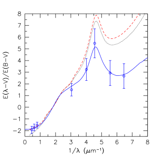
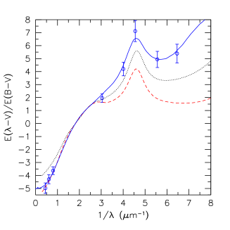
Figure 1: Left panel: Extinction data of HD 168785 (open circles) compared with our best-fit dust model (see Section 3),(blue) continuous line, and the best-fit standard CCM curves corresponding to the whole spectral range (black) dotted line, and to the IR data only, (red) dashed line. Right panel: Extinction data of BD+58 310 (open circles) compared with our best-fit dust model (blue) continuous line, and the corresponding best-fit standard CCM curves with the same symbols as in the left panel.

3 Models

Models of the extinction curves have been computed according to the prescriptions of Weingartner & Draine (2001) and Draine & Li (2007). The novelty of such models is that the grain size distribution is based on more recent observational constraints in the optical and infrared spectral domains (see Weingartner & Draine (2001) and references therein). Such distribution, a revision of the Mathis et al. (1977) size distribution (see Clayton et al. (2003) for a discussion on grain size distribution history), accounts for two populations of spherical grains: amorphous silicate (Si) and carbonaceous grains (C), the latter consisting of graphite grains and polycyclic aromatic hydrogenated (PAH) molecules. Their optical properties, which depend on their geometry and chemical composition, are described by Li & Draine (2001b, a) and by Draine & Li (2007), and account for new laboratory data i.e., the near-IR absorption spectra measured by Mattioda et al. (2005), as well as the spectroscopic observations of PAH emission from dust in nearby galaxies (Draine & Li (2007), and references therein).

The Weingartner & Draine (2001) size distribution (see their eq. 4) allows both for a smooth cutoff for grain size $a>a_{t}$, and for a change in the slope $d\,ln\,n_{gr}/d\,ln\,a$ for $a<a_{t}$. This requires several parameters which can be determined by the comparison with the observed curve, the comparison being performed with the Levenberg-Marquardt algorithm (Weingartner & Draine 2001). Table LABEL:parmod presents the size distribution parameters derived from our best-fit dust models of type C extinction curves where: b_C is the abundance of carbon (per H nucleus) in the double log-normal very small grain population (see Table 2 and eq. 12-14 of Draine & Li (2007)), $\alpha_{g}$ and $\alpha_{s}$ are the power law indexes of carbon and Si grain size distributions respectively, $\beta_{g}$ and $\beta_{s}$ their curvature parameters, a_t,g and a_t,s their transition sizes, a_c,g and a_c,s their upper cutoff radii. Such models, indeed, depend on ten parameters since a_c,s results to be constant (Weingartner & Draine (2001), Paper I). Fig. 1 compares the observed extinction curves of two type C lines with the corresponding best-fit models.
The values of such parameters able to reproduce the observed wavelength-dependent extinction law in the local Milky Way (MW), i.e. the observational fits of Fitzpatrick (1999) for R_V values 3.1, 4.0, and 5.5 and different b_C amounts, corresponding to twenty-five models, are derived by Weingartner & Draine (2001) (Fig.s 8-12; see also Draine (2003)). Li & Draine (2002) showed that these grain models are also consistent with the observed IR emission from diffuse clouds in the MW and in the SMC. The observational fits of Fitzpatrick (1999), in their turn, well agree with standard CCM curves for the same R_V values until R_V is smaller than 5.5 (Fitzpatrick 1999, his Fig. 7). Moreover, as pointed out in Paper 1, the extinction curves of Weingartner & Draine (2001) are almost unaffected by taking into account the more recent updating (Draine & Li 2007). Thus, WD models are useful tools to give insight into the properties of the dust trapped into the grain along normal lines or small deviating extinction lines (i.e. $<$2 $\sigma$). However, since the majority of R_V values in Table LABEL:anom0 are smaller than 3.1, a new set of WD parameters able to fit normal, CCM, curves with total-to-selective extinction coefficients from 2.9 and 2.0, have been computed and listed in Table 3 for each pair of values (R_V, b_C), as in Weingartner & Draine (2001). The last two columns of such a Table show volumes of carbonaceous and silicate populations normalized to their abundance/depletion-limited values, i.e. 2.07$\times$ 10^-27 cm^-3 H^-1 and 2.98$\times$ 10^-27 cm^-3 H^-1, respectively (Weingartner & Draine 2001). As discussed by Draine (2003) and Draine (2004), models in Table 1 of Weingartner & Draine (2001) slightly exceed the abundance/depletion-limited values of silicon grains ($\leq$20%) and we assume such a value as the maximum allowed. Fig. 2 shows two normal curves of our sample with small R_V, their best-fit standard CCM curves and, as a comparison, WD dust grain models to fit the data. Properties of all these models, both of normal and of anomalous curves, are given in the next section in terms of dust-to-gas ratios, abundance ratios, and small-to-large grain size ratios of the dust trapped into the grains along such extinction curves.
There are several distinct interstellar dust models that simultaneously fits the observed extinction, infrared emission, and abundances constraints (Zubko et al. 2004). Models of WD allow us to compare the results of our deviating curves here with those of normal curves, in a self-consistent framework.

Table 3: Best-fit parameters of WD grain size distributions for CCM curves with small R_V values

RV	$10^{5}b_{C}$	$\alpha_{g}$	$\beta_{g}$	at,g	ac,g	Cg	$\alpha_{s}$	$\beta_{s}$	at,s	Cs	V${}_{g}^{C}$	V${}_{g}^{Si}$
				$(\mu m)$	$(\mu m)$				$(\mu m)$
2.9	0.0	-1.90	-0.97	0.008	0.450	1.96$\times 10^{-10}$	-2.32	0.35	0.168	7.85$\times 10^{-14}$	0.74	1.04
2.9	1.0	-1.96	-0.71	0.007	0.650	1.62$\times 10^{-10}$	-2.32	0.47	0.166	7.50$\times 10^{-14}$	0.66	1.04
2.9	2.0	-1.90	-0.51	0.006	0.597	1.82$\times 10^{-10}$	-2.32	0.47	0.168	7.85$\times 10^{-14}$	0.80	1.11
2.9	3.0	-1.77	-0.20	0.008	0.760	2.70$\times 10^{-11}$	-2.36	0.60	0.153	7.50$\times 10^{-14}$	0.82	0.98
2.9	4.0	-1.75	-0.23	0.008	0.760	4.00$\times 10^{-11}$	-2.37	0.60	0.163	7.50$\times 10^{-14}$	1.00	1.17
2.6	0.0	-2.45	-0.12	0.013	0.705	2.10$\times 10^{-11}$	-2.41	0.39	0.148	7.00$\times 10^{-14}$	0.55	0.79
2.6	1.0	-2.36	-0.10	0.012	0.500	2.10$\times 10^{-11}$	-2.41	0.39	0.155	7.00$\times 10^{-14}$	0.60	0.90
2.6	2.0	-2.30	-0.08	0.012	0.500	1.51$\times 10^{-11}$	-2.40	0.39	0.155	7.00$\times 10^{-14}$	0.56	0.89
2.6	3.0	-2.30	-0.04	0.012	0.250	1.51$\times 10^{-11}$	-2.40	0.44	0.165	7.00$\times 10^{-14}$	0.57	1.07
2.6	4.0	-2.15	0.01	0.012	0.187	1.01$\times 10^{-11}$	-2.40	0.44	0.165	7.00$\times 10^{-14}$	0.57	1.07
2.6	5.0	-2.10	0.03	0.012	0.187	1.01$\times 10^{-11}$	-2.40	0.39	0.158	8.75$\times 10^{-14}$	0.71	1.16
2.3	0.0	-2.65	-0.18	0.014	0.705	1.65$\times 10^{-11}$	-2.40	0.32	0.158	7.00$\times 10^{-14}$	0.41	0.90
2.3	0.5	-2.60	-0.15	0.014	1.050	1.50$\times 10^{-11}$	-2.420	0.22	0.155	1.50$\times 10^{-13}$	0.47	0.96
2.3	1.0	-2.75	-0.17	0.012	0.705	1.50$\times 10^{-11}$	-2.42	0.42	0.155	7.00$\times 10^{-14}$	0.42	0.91
2.3	2.0	-2.55	-0.10	0.011	0.705	1.65$\times 10^{-11}$	-2.30	0.34	0.158	7.00$\times 10^{-14}$	0.36	0.90
2.3	3.0	-2.15	-0.27	0.012	0.700	1.60$\times 10^{-11}$	-2.44	0.48	0.147	8.00$\times 10^{-14}$	0.48	0.93
2.3	4.0	-2.10	-0.20	0.010	0.980	1.97$\times 10^{-11}$	-2.44	0.45	0.145	9.80$\times 10^{-14}$	0.62	1.10
2.3	5.0	-2.10	-0.08	0.011	0.988	1.13$\times 10^{-11}$	-2.47	0.65	0.143	9.80$\times 10^{-14}$	0.69	1.17
2.0	0.0	-2.12	-1.86	0.009	0.105	9.30$\times 10^{-11}$	-2.37	0.09	0.146	5.60$\times 10^{-14}$	0.17	0.49
2.0	1.0	-2.00	-0.99	0.010	0.150	2.98$\times 10^{-11}$	-2.38	0.03	0.147	5.60$\times 10^{-14}$	0.24	0.48
2.0	2.0	-1.95	-0.50	0.009	0.450	1.50$\times 10^{-11}$	-2.46	0.37	0.136	6.00$\times 10^{-14}$	0.24	0.55
2.0	3.0	-1.95	-0.30	0.008	0.450	1.30$\times 10^{-11}$	-2.52	0.65	0.136	6.00$\times 10^{-14}$	0.27	0.65
2.0	4.0	-1.95	-0.30	0.010	0.450	1.30$\times 10^{-11}$	-2.65	1.25	0.136	6.00$\times 10^{-14}$	0.42	0.92
2.0	5.0	-1.95	-0.30	0.013	0.450	1.30$\times 10^{-11}$	-2.70	1.70	0.136	6.00$\times 10^{-14}$	0.46	1.09

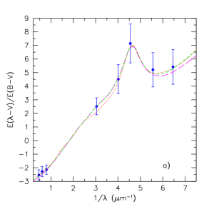
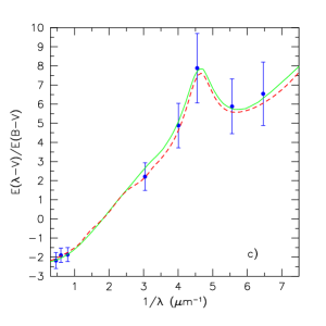
Figure 2: Panel a): HD 39136, a normal curve of our sample (blue filled squares) whose best-fit standard CCM curve corresponds to R_V= 2.85$\pm$0.47 (red dotted line). The (magenta) long-dashed line is computed as the seventh model in Table 1 of Weingartner & Draine (2001), R_V=3.1, including latest updating (Draine & Li 2007); the (green) short-dashed line is our best-fit dust model: the fifth model in Table 3. Panel b): HD 12323, a normal curve of our sample (blue filled squares) whose best-fit standard CCM curve corresponds to R_V= 2.30$\pm$0.51 (red dashed line); the (green) continuous line is the best-fit dust model: the thirteenth model in Table 3.

4 Results

For a given chemical composition of the grains, the total volume occupied by the dust grains, $V_{g}$, which includes the total volume per hydrogen atom of each grain type, is directly connected with the dust-to-gas ratio, $\rho_{d}/\rho_{H}$, as described in eq.s 3, 4, 5, and 6 of Paper I i.e.:

$$\frac{\rho_{d}}{\rho_{H}}=\frac{\rho_{g}}{m_{H}}\frac{V_{g}}{n_{H}}=\frac{4\pi}{3m_{H}N_{H}}\sum_{X}\rho_{X}\int_{a_{min}}^{a_{max}}a^{3}N_{X}(a)da$$ (3)

where the integral is computed for the size distributions of the grains, i.e., from parameters in Table LABEL:parmod for anomalous curves and, for normal curves, both in Table 1 of Weingartner & Draine (2001), however accounting for latest updating (Draine & Li 2007), and in Table 3.

The number of atoms of an element per interstellar H nucleus trapped in the grains i.e, the C/H and Si/H abundances, and the same fractions compared with the solar values i.e., C/C_⊙ and Si/Si_⊙, can be computed from the $\rho_{d}/\rho_{H}$ ratio of each type of grains. The solar values of carbon and silicon dust abundances adopted at this aim are, as in Paper I, (C/H)${}_{\odot}=3.3\times 10^{-4}$, (Si/H)${}_{\odot}=3.65\times 10^{-5}$; the average mass in our own galaxy of one carbon grain is 19.93$\times$10^-24 gr/cm^-3 and that of one silicon grain 28.7$\times$10^-23 gr/cm^-3, as in Weingartner & Draine (2001); such values are in good agreement with recent estimates by Clayton et al. (2003): (C/H)${}_{\odot}=3.2\times 10^{-4}$ and (Si/H)${}_{\odot}=4.0\times 10^{-5}$.
The properties of the grains along type A and B anomalous curves, investigated in Paper I, show that B curves are characterized by a number of small silicon grains lower than normal curves with the same R_V, and lower than A curves too; they are also characterized by a larger number of small carbon grains as A curves are. Such results, here revised accounting for recent updating of Draine & Li (2007), are included in the figures to allow comparisons. The main change of such improvements (Table 2 of Draine & Li (2007)), is related to the number of carbon atoms per total H in each of the log-normal components (eq.s 11-14 of Draine & Li (2007)). Appreciable effects occur when the parameters of grain size distribution provide a larger number of small carbon grain than the number required to fit normal lines, thus in the case of anomalous lines.

In the figures, error bars of WD normal curves span the range of values of different models corresponding to the same R_V value (Section 3).

The results of our WD best-fit models of type C curves are reported in Table LABEL:resanom1: the name of sight line is in col. I, the dust-to-gas ratio in unit of 10^-2 in col. II, the abundance ratios in col. III and IV, the small-to-large grain size ratios of carbon, R_C, in col. V and of silicon grains, R_Si, in col. VI, the R_V value in col. VII, and the E_(B-V)/N_H ratio in col. VIII. Here, as in the following, we define small grains those with size $a\leq 0.01\,\mu$m, and large grains those with size above such a value.

The following conclusions can be derived by comparing the results presented in Table LABEL:resanom1 with those derived from the same dust grain models of normal extinction curves (Section 3):

i) Dust population models generally imply substantial abundances of elements in grain material, approaching or exceeding the abundances believed to be appropriate to interstellar matter (Draine 2003, and references therein). It is remarkable that, according to our models, the predicted amount of carbon that condenses into grains along the majority of our sight lines is lower than the average galactic value (Fig. 3). Only three anomalous curves, HD 37061, HD 21455, and HD 164492, require C/H abundance larger than the solar value. Moreover, for about 74% of our models of type C curves, the predicted C/H ratio does not exceed a fraction 0.7-0.6 of C cosmic abundance which is accepted, although with large uncertainties, as the average amount of carbon trapped in grains (Draine 2009). No anomalous line model exceeds the solar value of the silicon abundance.

ii) The dust-to-gas ratio of type C curves is linked to the E(B-V)/N(H) ratio by the relation:

$$\frac{\rho_{d}}{\rho_{H}}=(0.2730\pm 0.019)\times\frac{E(B-V)}{N_{H}}+(+0.020\pm 0.021)$$ (4)

with dispersion 0.076 (dashed line in Fig. 4) and E(B-V)/N(H) in units of the average Galactic value, i.e., 1.7$\times 10^{-22}$ mag cm² (Bohlin et al. 1978). Accounting for all our anomalous curves we derive:

$$\frac{\rho_{d}}{\rho_{H}}=(0.377\pm 0.018)\times\frac{E(B-V)}{N_{H}}+(-0.043\pm 0.025)$$ (5)

with dispersion 0.13, (continuous line in Fig. 4), in well agreement with the results of Paper I, although with a slightly smaller correlation index, 0.92 instead of 0.95.

Therefore, anomalous curves are characterized by dust-to-gas ratios lower than the average galactic value. In particular no type C extinction curve exceeds the critical galactic value, 0.01 (Barbaro et al. 2004, and references therein), independently of its carbon grain abundance (see i)). Extinction curves of our sample having E(B-V)/N(H) ratio equal to the average Galactic value, exhibit their anomalous character due to a dust-to-gas ratio lower than normal curves. Moreover, their E(B-V)/N(H) can be affected by modifying the dust-to-gas ratio without any relevant change in R_V unlike the behavior expected for normal extinction curves (Fig. 5, left panel).

So, while anomalous curves can arise also in environments with normal reddening properties, strong deviations from the average reddening Galactic value are a signature of anomaly as shown in Fig. 5, right panel, and discussed in Barbaro et al. (2004).

iii) In the large majority of the cases, the expected small-to-large grain size ratios of anomalous lines differ from the corresponding values expected for WD CCM curves (Fig. 6). Anomalous curves are generally characterized by a number of small carbonaceous grains larger than normal curves whereas the small-to-large size ratios of Si grains span a wider range, from lower up to larger values than normal lines. Only five anomalous curves have normal values of both these ratios, BD+59 2829 and BD+58 310, belonging to the 2$\delta$ sample, and HD 14707, HD 282622, BD+52 3122, to the 3$\delta$ sample. For these sightlines their best-fit standard CCM curve in the UV range is below the observed data, as outlined in Section 2 (Fig. 1, right-panel).

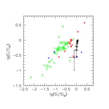
Figure 3: Abundances of the dust locked up into the grains along our anomalous sight lines compared with the solar values (see text); (green) open circles are for type C curves, (black) squares are for normal curves computed with WD parameters corresponding to seven different R_V values, i.e. forty-nine models (Section 3). Also included are the results of type A and B extinction models (Paper I), (red) stars and (blue) filled triangles respectively, here revised accounting for latest updating (Draine & Li 2007) (see text).

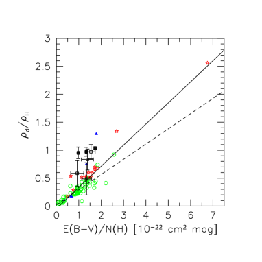
Figure 4: The behavior of the dust-to-gas ratio, $\rho_{d}/\rho_{H}$, normalized to the average Galactic value, 0.01, with the E(B-V)/N_H ratio in unit of $1.7\times 10^{-22}$ mag cm² (Bohlin et al. 1978); symbols are as in the previous figure. The dashed line shows the relation for type C curves (eq. 4) and the continuous line that for all the anomalous curves analyzed (eq. 5).

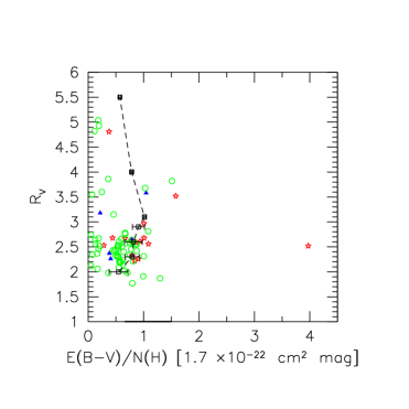
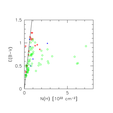
Figure 5: Left panel: The R_V values and the corresponding E(B-V)/N_H ratios in unit of $1.7\times 10^{-22}$ mag cm², as derived from our WD dust grain models (see text); symbols are as in the previous figures; the dashed line connects the results of WD models of normal curves corresponding to seven different R_V values (Section 3); the range in bold-face on x-axis shows the expected deviation of galactic curves (Bohlin et al. 1978). Right panel: The behavior of the reddening, E(B-V) (Savage et al. 1985), as a function of the predicted total hydrogen column density; continuous line shows the galactic average relationship found by analyzing a large sample of sight lines whose HI and H₂ column densities were measured: E(B-V)/N(H)=1.7$\times 10^{-22}$ mag cm² (Bohlin et al. 1978); symbols are the same as in the previous figures.

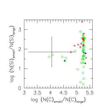
Figure 6: The predicted small-to-large grain size ratios for carbonaceous and silicate grains of anomalous sight lines compared with the range spanned by WD models of CCM curves (continuous lines) for the same range of R_V values.

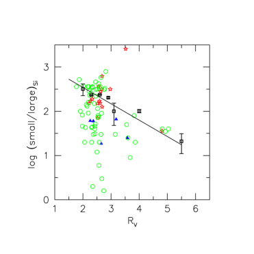
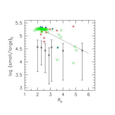
Figure 7: The expected behavior of the small-to-large grain size ratio of silicate and carbonaceous dust against R_V values along anomalous sight lines compared with the same along CCM curves (open squares) computed with WD parameters (Section 3). Continuous line in the left panel corresponds to the relationship: y=(-0.37$\pm$0.03)+(3.30$\pm$0.09), with dispersion 0.18 and anti-correlation index -0.91, that applies to normal lines. Continuous line in the right panel shows the relationship for the whole sample of anomalous curves: y=(-0.25$\pm$ 0.03)x $+$( 5.83$\pm$0.09) with dispersion 0.19 and correlation index -0.65.

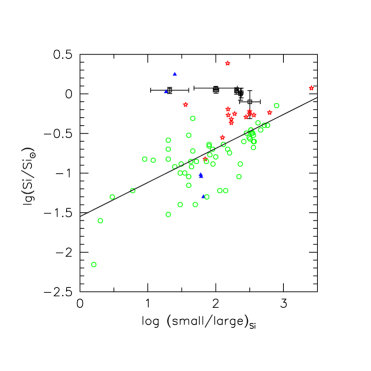
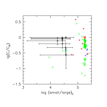
Figure 8: The expected behavior of the small-to-large grain size ratio of silicate (left panel) and carbonaceous dust (right panel) against the silicon and carbonaceous dust abundances of anomalous sight lines; continuous line holds for Si grains of the whole sample: y=(0.43$\pm$0.06)x$+$(-1.55$\pm$0.13) with dispersion 0.34 and correlation index 0.60. Symbols are the same as in the previous figures.

iv) The small-to-large size ratio of Si grains is almost independent of the selective extinction coefficient, R_V (r=-0.20), unlike the normal curves. For such curves this ratio anti-correlates strongly with R_V (Fig. 7, left panel). The same ratio of carbon grains for type C curves is, indeed, anti-correlated with R_V with anti-correlation index r=-0.80, at a variance with WD CCM lines (Fig.7, right panel). Such anti-correlation is somewhat weakened by including all the anomalous curves in the sample.

v) From the analysis of Fig. 8, left panel, the small-to-large size ratio of Si grains along anomalous lines is correlated with the Si abundance (continuous line in Fig. 8); type C curves are more correlated (r=0.73). The models predict Si abundances up to hundred times lower than solar values.

Compared with the characteristics of the environments where other types of lines of sight occur, those typical of C types present, in average, the behavior summarized below and reported in Table 5, where the mean values and their errors are in the same units as in Table LABEL:resanom1; N indicate WD normal curves:

1) The small-to-large size ratio of carbonaceous grains is almost six times higher than the average value found for normal curves and it is comparable to the average value of type A and B curves.

2) The small-to-large size ratio of silicon grains is smaller than the average value of A types and almost three times larger than that of type B curves, however it is like that of normal curves.

3) The average amount of carbon which condenses into grains is slightly lower than the expected galactic abundance trapped into grains, 0.7-0.6; that is the value of normal curves as derived here from the same grain models. Type A reaches the maximum value allowed; this is almost three times larger than that of B curves which show the lower value.

4) All the anomalous curves show Si abundance lower than that of normal curves; type C, in particular, is characterized by the lowest amount.

Therefore, type C sight lines require, in average, dust abundances lower than the abundances trapped into the grains along normal lines, in particular of silicate grains, as well as small-to-large grain size ratios of carbonaceous dust larger than expected for normal curves. Such properties are different from those expected for A and B curves. The former, in particular, correspond to sight lines with the highest abundances of carbonaceous dust and the latter ones to lines of sight with both the lowest carbon abundances and the lowest small-to-large grain size ratio of silicon dust, i.e., the largest Si grains.

The different properties of the dust locked into the grains along anomalous sight lines can be recovered accounting for the violent nature of the interstellar medium. Shocks and grain-grain collisions should both destroy dust grains, so reducing the amount of the dust trapped in the grains, and modify the normal size distribution of the dust increasing the small-to-large grain size ratio, as it will be discussed in the next section.

Table 5: Average properties of the dust locked up into the grains of WD extinction models

T	$\frac{\rho_{d}}{\rho_{H}}$	$\frac{R_{C}}{10^{4}}$	$\frac{C}{C_{\odot}}$	$\frac{R_{Si}}{10^{2}}$	$\frac{Si}{Si_{\odot}}$
A	0.72$\pm$0.15	15.8$\pm$1.13	1.00$\pm$0.22	3.79$\pm$1.61	0.68$\pm$0.14
B	0.50$\pm$0.23	17.5$\pm$3.54	0.35$\pm$0.03	0.46$\pm$0.10	0.61$\pm$0.34
C	0.28$\pm$0.02	16.4$\pm$0.59	0.56$\pm$0.05	1.69$\pm$0.22	0.20$\pm$0.02
N	0.86$\pm$0.03	2.8$\pm$0.32	0.71$\pm$0.03	1.58$\pm$0.14	1.04$\pm$0.03

5 Discussion

Table LABEL:FMpar presents the values of the Fitzpatrick & Massa (1988, 1990) parameters (FM parameters in the following) of type C curves derived from our models, since a right estimate of such parameters from only five UV color excesses is impossible.

Then, the properties of our sample can be compared with those of Valencic et al. (2004), the larger and homogeneous sample of galactic extinction curves with known FM parameters and R_V values available so far. Valencic et al. (2004) found that the CCM extinction law, with suitable R_V values, applies for 93$\%$ of their 417 sight lines and that only four lines deviate by more than 3$\sigma$. They conclude that the physical processes that give rise to grain populations that have CCM-like exctinction dominate the interstellar medium.

Sixteen of curves here have been studied also by Valencic et al. (2004), five belonging to the 3$\delta$ sample, HD 14357, HD 37061, HD 164492, HD 191396, BD$+$57 252, and eleven to the 2$\delta$ sample, HD 54439, HD 96042, HD 141318, HD 149452, HD 152245, HD 168137, HD 248893, HD 252325, BD$+$59 2829, BD$+$62 2154, and BD$+$63 1964. By comparing their parameterized UV extinction curves at the five ANS wavelengths with our ones, we find meaningful differences, i.e., larger than three $\sigma_{r}$ at one wavelength or more, for all the common curves of the 3$\delta$ sample, unless for BD$+$57 252 which well agrees with our data. Concerning the sight lines belonging to the 2$\delta$ sample, three curves (i.e., HD 168137 and HD 252325, and HD149452) show differences larger than two $\sigma_{r}$ at four wavelengths, one curve (i.e., HD 248893) at two wavelengths and four curves (i.e., HD 152245, BD$+$59 2829, BD$+$62 2154, and BD$+$63 1964) at one wavelength. HD 96042 well agrees with our data, and the remaining curves, i.e., HD 54439 and HD 141318, show only differences lower than two $\sigma_{r}$ at one wavelength.

It must be remarked, however, that spectral type and luminosity class of Valencic et al. (2004) are based on spectral properties in the UV rather than in the visible spectral range as in Savage et al. (1985); moreover the color excesses used by Valencic et al. (2004) are derived from IUE (International Ultraviolet Explorer) spectra using the pair method, whereas Savage et al. (1985) used the ANS photometry and intrinsic colors by Wu et al. (1980) as described in Section 2.

Fig 9 compares the FM parameters of sixtheen common sight lines here together with those (eight) in Paper 1.

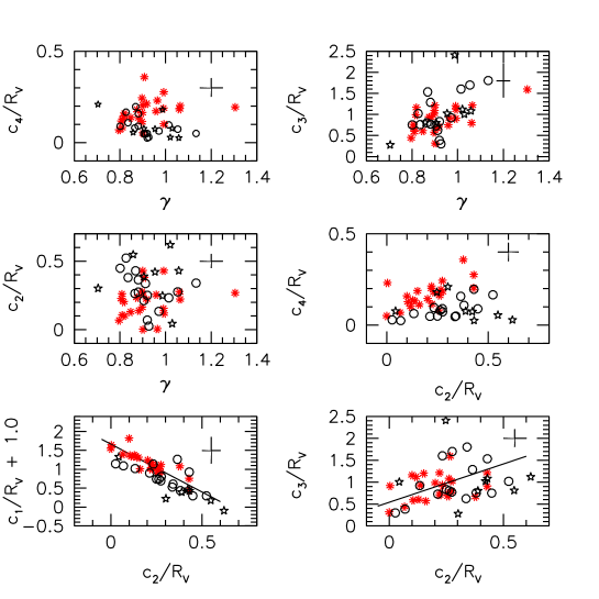
Figure 9: Open circles and stars (black) show the FM parameters of sixteen extinction curves derived from our best-fit dust models in Section 3 together with those of eight curves in Paper 1, respectively; asterisks (red) are for the same curves by Valencic et al. (2004); continuous lines show the relations as derived by Valencic et al. (2004) (see their Table 6).

5.1 The FM parameterization

In the following we define $c^{\prime}_{i}=c_{i}/R_{V}$ for i=2,3, and 4, $c^{\prime}_{1}=c_{1}/R_{V}+1$, $x_{o}$ and $\gamma$ being the same, to compare our results with those of Valencic et al. (2004). The data in Table LABEL:FMpar concern the parameterization in terms of the normalized color excesses, i.e., $\kappa(\lambda)$=E($\lambda$-V)/E(B-V), whereas the primed symbols, i.e., $c^{\prime}_{i}$, are in term of A($\lambda$)/A_V. Fig.s 10, 11, and Fig. 12, compare the FM parameters of all our anomalous curves with both the FM parameters derived from WD CCM curves (Section 3), and the sample of Valencic et al. (2004, their Table 5).

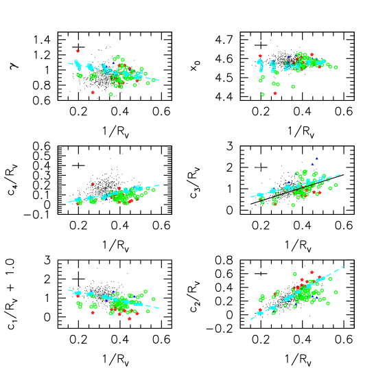
Figure 10: Black points show the FM parameters of extinction curves in Valencic et al. (2004); open circles (green) are the FM parameters of C type anomalous curves as derived from our models (see Sect. 3), (red) stars and (blue) triangles are the same of A and B types, and (cyan) open squares of WD CCM models (see text); black continuous lines are the relationships in Table 8 with r$>$0.50, (cyan) dashed lines are the same for WD CCM curves (Table 6).

Figures 10, 11, and Fig. 12 show the relations between the different parameters. Relationships with (anti)/co-relation index, r, larger than (-)0.4 are reported in Table 6 for WD normal CCM curves, in Table 7 for C types, and in Table 8 for all the anomalous sight lines.

Looking at Fig.s 10, 11, and Fig. 12 important agreements with the results of Valencic et al. (2004) are emphasized as well as similar trends as WD normal curves. These points show that dust models of anomalous curves, which best-fit ANS data, are not biased by the low resolution of such data. In particular:

Table 6: Relations between FM parameters of WD CCM curves

r	linear fit	dispersion
$-$0.98	$c^{\prime}_{1}=(-2.177\pm 0.264)/R{{}_{V}}+(1.746\pm 0.022)$	0.0428
+0.99	$c^{\prime}_{2}=(1.731\pm 0.020)/R{{}_{V}}-(0.331\pm 0.007)$	0.013
+0.97	$c^{\prime}_{3}=(2.409\pm 0.092)/R{{}_{V}}-(0.246\pm 0.032)$	0.060
+0.96	$c^{\prime}_{4}=(0.394\pm 0.016)/R{{}_{V}}+(0.032\pm 0.006)$	0.010
$-$0.87	$\gamma=(-0.508\pm 0.041)/R{{}_{V}}+(1.166\pm 0.014)$	0.027
$-$0.99	$c^{\prime}_{1}=(-1.269\pm 0.024)c^{\prime}_{2}+(1.333\pm 0.007)$	0.028
$-$0.90	$c^{\prime}_{4}=(-0.628\pm 0.045)\gamma+(0.726\pm 0.045)$	0.017
+0.96	$c^{\prime}_{3}=(1.375\pm 0.057)c^{\prime}_{2}+(0.711\pm 0.017)$	0.065
+0.96	$c^{\prime}_{4}=(0.226\pm 0.009)c^{\prime}_{2}+(0.044\pm 0.003)$	0.010
-0.86	$c^{\prime}_{2}=(-2.577\pm 0.216)\gamma+(2.816\pm 0.216)$	0.010
-0.79	$c^{\prime}_{3}=(-3.380\pm 0.374)\gamma+(4.420\pm 0.374)$	0.143
+0.93	$c^{\prime}_{3}=(5.664\pm 0.321)c^{\prime}_{4}+(0.488\pm 0.034)$	0.086
+0.96	$c^{\prime}_{4}=(0.083\pm 0.003)c^{\prime}_{3}\pi/2\gamma^{2}+(0.040\pm 0.006)$	0.011

Table 7: Relations between FM parameters of type C anomalous curves

r	linear fit	dispersion
+0.61	$c^{\prime}_{3}=(3.086\pm 0.511)/R{{}_{V}}+(-0.209\pm 0.208)$	0.300
+0.61	$c^{\prime}_{4}=(0.330\pm 0.054)/R{{}_{V}}-(0.047\pm 0.022)$	0.032
+0.60	$x_{o}=(0.320\pm 0.054)/R{{}_{V}}+(4.432\pm 0.022)$	0.032
$-$0.83	$c^{\prime}_{1}=(-2.219\pm 0.186)c^{\prime}_{2}+(1.379\pm 0.058)$	0.144
$-$0.48	$c^{\prime}_{4}=(-0.224\pm 0.053)\gamma+(0.297\pm 0.049)$	0.035
+0.43	$c^{\prime}_{4}=(0.173\pm 0.047)c^{\prime}_{2}+(0.034\pm 0.015)$	0.036
+0.53	$x_{o}=(0.246\pm 0.048)\gamma+(4.338\pm 0.045)$	0.034
+0.68	$c^{\prime}_{3}=(3.021\pm 0.417)\gamma-(1.767\pm 0.386)$	0.278
+0.76	$x_{o}=(+0.080\pm 0.009)c^{\prime}_{3}+(4.483\pm 0.010)$	0.026

Table 8: Relations between FM parameters of all the anomalous curves

r	linear fit	dispersion
+0.55	$c^{\prime}_{3}=(3.064\pm 0.515)/R{{}_{V}}+(-0.183\pm 0.207)$	0.344
+0.44	$c^{\prime}_{4}=(0.262\pm 0.059)/R{{}_{V}}-(0.019\pm 0.024)$	0.040
+0.48	$x_{o}=(0.262\pm 0.054/R{{}_{V}}+(4.464\pm 0.022)$	0.036
$-$0.88	$c^{\prime}_{1}=(-2.326\pm 0.142)c^{\prime}_{2}+(1.405\pm 0.047)$	0.149
$-$0.54	$c^{\prime}_{4}=(-0.248\pm 0.043)\gamma+(0.315\pm 0.040)$	0.037
+0.62	$x_{o}=(0.263\pm 0.037)\gamma+(4.322\pm 0.035)$	0.032
+0.55	$c^{\prime}_{3}=(2.331\pm 0.399)\gamma-(1.145\pm 0.374)$	0.346
+0.67	$x_{o}=(+0.067\pm 0.008)c^{\prime}_{3}+(4.499\pm 0.009)$	0.030

i) The correlation between c${}^{\prime}_{3}$, the bump height, and 1/R_V for the whole sample exhibits the same slope as both WD normal curves (Table 6) and the sample of Valencic et al. (2004), that shows the same correlation index as our sample (slope 3.48$\pm$0.24, and dispersion 0.25).

Indeed each type of anomalous curve obeys a different relation: B curves show the stronger correlation index (r=0.99) and the steeper slope (6.77$\pm$0.46); A curves have an intermediate correlation index, r=0.64, but the lower slope 2.10$\pm$0.64.

ii) $\Gamma$, the full width at half maximum (FWHM) of the bump, spans a large range of values by changing 1/R_V as the sample of Valencic et al. (2004), perhaps reflecting a wide range of environments (Cardelli & Clayton 1991). No correlation is found for our sample as well as for each anomalous type, unlike WD CCM models.

iii) For the whole sample of anomalous curves, c${}^{\prime}_{4}$, the far-UV (FUV) non linear rise, and 1/R_V correlate with a lower correlation index than WD normal curves but almost with the same slope; B types are better correlated (r=0.87) than C types, whereas A types do not correlate (r=-0.20). The sample of Valencic et al. (2004) shows a weaker correlation, r=0.38, and a higher slope, 0.51$\pm$0.06, than our findings for the total sample.

iv) The correlation between $c^{\prime}_{2}$ and $c^{\prime}_{1}$ (Fig. 11) shows how tightly constrained are the linear components of the extinction. The whole sample of anomalous curves is more strongly correlated (Table 8) than type C curves (Table 7). Their slope agrees within the errors with the findings of Valencic et al. (2004, their Table 6) but it is steeper than that derived from WD CCM models, more than three times the error. As discussed in the previous section, this difference is a consequence of the lower amount of dust grains with normal and large sizes which affects the optical portion of the extinction curve of anomalous sight lines compared to normal lines.

v) The parameters $c^{\prime}_{4}$ and $c^{\prime}_{2}$ do not correlate (r=0.17) for the whole sample of anomalous curves, in agreement with the findings of Valencic et al. (2004, and references therein). Thus the carriers of the FUV non-linear rise are not the same as the optical linear rise. For WD CCM curves such parameters, indeed, are correlated. A weak correlation arises for C types (Table 7).

vi) Our results between $c^{\prime}_{2}$ and $\gamma$ (r=-0.31) are in agreement with those Valencic et al. (2004, and references therein) which do not find any correlation. For WD CCM models such parameters are anti-correlated, wider bumps are found in extinction curves with weaker linear rises.

vii) For the whole sample of anomalous curves we find the same correlation between $c^{\prime}_{3}$ and $\gamma$ as that of Valencic et al. (2004) (Table 8), with a correlation index slightly lower than their (their Table 6, r=0.58). It means that as the bump FWHM increases, the bump strength is also increasing. C types are better correlated and with a steeper slope than the whole sample here. Jenniskens & Greenberg (1993) attributed this relation, at least partly, to the fitting procedure whereas, following Fitzpatrick & Massa (1988), such parameters are truly related in some way. WD CCM curves span a shorter range of $\gamma$ and $c^{\prime}_{3}$ values which are anti-correlated.

viii) There is almost no correlation between $c^{\prime}_{4}$ and $c^{\prime}_{3}$ for both the whole sample (r=0.24) and type C curves (r=0.25), as well as for the sample of Valencic et al. (2004) (r=0.31), whereas the correlation is strong for WD CCM curves. As discussed in Paper I, A types are weakly anti-correlated (r=-0.56) and B types are strongly correlated (r=0.92).

Therefore, looking at the same figures, several important differences arise from our sample and that of Valencic et al. (2004).

i) There is a weak relation between $x_{o}$, the bump position ($\mu m^{-1}$), and 1/R_V that is stronger for type C curves, at a variance with the results both of Valencic et al. (2004) and of WD CCM models (r=0.31).

ii) For the whole sample of anomalous curves $c^{\prime}_{4}$ and $\gamma$ are anti-correlated in the sense that a broader bump is found along sight lines with smaller FUV non linear rise; by considering only type A curves, the anti-correlation index increases (r=-0.87) whereas, by considering only C types, the anti-correlation index decreases (Table 7). No correlation is found by Valencic et al. (2004) while Carnochan (1986), Fitzpatrick & Massa (1988), and Jenniskens & Greenberg (1993) obtained an opposite trend, in the sense that a wider bump is found along sight lines with larger FUV rise. It must be remarked that WD CCM curves show a very similar trend as anomalous curves although with a steeper slope and a higher anti-corelation index. This finding cannot be ascribed to the less well sampling in wavelength of ANS data since a similar trend arises from dust models fitting also complete extinction curves. This is provided by the different dust components that play the job in our models.

iii) The parameters $c^{\prime}_{2}$ and $c^{\prime}_{3}$ do not correlate for the whole sample of anomalous curves (r=-0.05) as well as for C types (r=0.06), at variance with the results of Valencic et al. (2004, their Table 6, r=0.49) and with those of WD normal curves. However, when considering separately type A and B curves good correlations are found though with very different slopes (Paper I). In particular, looking at Fig. 11, A and B curves outline the lower and upper limits of the region where C curves mix to normal ones. The correlation occurring separately for A and B types suggests that some fraction of the linear rise is associated with the bump (Carnochan 1986) but in a different proportion for such types, as discussed in Paper I. C type curves, characterized by intermediate properties of their grain populations compared with A and B types, as outlined in the previous section, have no the same proportion of grains which contribute to the bump and to the linear rise, thus do not correlate.

So, anomalous curves show bump properties, i.e., bump width, bump height, bump strength, $c^{\prime}_{3}/\gamma^{2}$, and bump position, well correlated whereas the same properties are independent of the linear rise $c^{\prime}_{2}$ (Fig. 12). Neither WD CCM models, neither the sample of Valencic et al. (2004) show any correlation with the bump position. Moreover, the bump height, $c^{\prime}_{3}$ correlates with the linear rise, $c^{\prime}_{2}$, both for the sample of Valencic et al. (2004) and for WD CCM models (Table 6), though with different slopes, showing that bump properties are driven by different dust components, contrary to what happens for anomalous curves.

WD models of normal curves show a good correlation between the bump area, $\pi c^{\prime}_{3}/(2\gamma)$, and the FUV non-linear rise, emphasizing that the same grain populations concur to these features, whereas C type curves show a weak correlation which weakens further by considering the whole sample of anomalous curves (r=0.40), since A types do not correlate (r=-0.28).

Therefore, several extinction properties of type C anomalous curves differ from those of CCM curves computed with the same dust models and corresponding to the same R_V values, showing that mechanisms working in the environments of anomalous curves are different from those in the environments of normal curves.

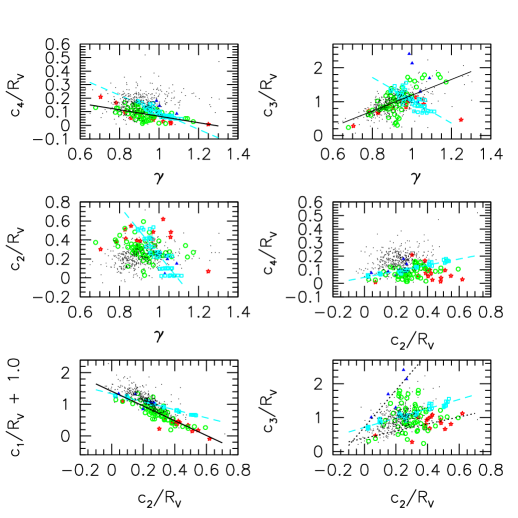
Figure 11: FM parameters of our extinction curves compared with the sample of Valencic et al. (2004); symbols are as in the previous figure; dotted lines in the bottom right panel are correlations for A and B types (Paper I).

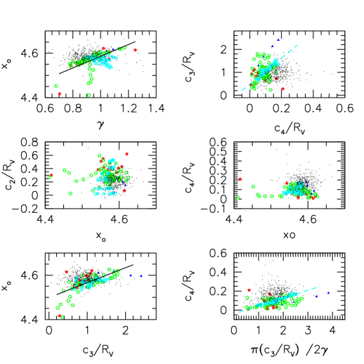
Figure 12: FM parameters of all our anomalous curves compared with the sample of Valencic et al. (2004); symbols are as in Fig. 10; dotted line is for B types and dashed line for A types, following Table 5 in Paper I.

5.2 Insight into environmental conditions

The results here derived from dust grain models (Weingartner & Draine 2001; Draine & Li 2007), show that the dust-to-gas ratios predicted for our sample are lower than the average galactic value (Section 4). For A types, in particular, the average value of such a ratio is the larger value, whereas for C types is the lower one. Such a trend is a consequence of the under abundance of Si grains, which, for A types, is in average 1.5 times less than that of normal, CCM curves computed with the same grain models. However it is at least three times greater than that of type C curves (Table 5). Moreover, the anomalous behavior of type C curves is driven by a larger population of small grains than the normal population, i.e., that characterizing lines of sight with extinction properties like CCM curves.

Many theoretical studies have faced the problem of the influence of shock waves on grains and their size distributions (Jones (2009a, b) and Draine (2009) for a review). As much as 5%-15% of the initial grain mass (a $\geq 0.005\,\mu$m) may be end up in very small fragments with a$\simeq.0014\,\mu$m in shock waves expanding in a warm interstellar medium with shock velocities between 50 and 200 km/s (Jones et al. 1996). High velocity shocks affect grains through sputtering reducing the number of small particles, while in shocks with lower velocities grain-grain collisions alter the size distribution by increasing the small-to-large grain size ratio (Jones 2005). Following Cowie (1978), silicate grains may be almost destroyed by velocity shock higher than $\simeq$80 Km/s while graphite grains require velocities higher than 100 Km/s. Jones et al. (1996) found that, for a shock velocity of 100 Km/s, the percentage of the initial mass of silicate grains destroyed increases from 18% to 37% by increasing the average density of the pre-shock gas, $n_{0}$, from 0.25 to 25 cm^-3; for the same conditions, that of destroyed carbonaceous grains increases from 7% to 13%. Detailed description of the various grain destruction mechanisms and grain lifetime in the interstellar medium were presented by Jones et al. (1996) and Jones (2004). Moreover, with shocks having high velocities, the destruction of silicate grains by sputtering can reduce the depletion of Si (Barlow & Silk 1977). Recently, Guillet et al. (2009) found that silicon dust is destroyed in J-type shocks slower than 50 Km/s by vaporisation not sputtering.

In order to gather information on the physical nature and the behavior of grains, the knowledge of the environments crossed by the sightlines is as much essential as the shape of the extinction curves. Unfortunately the knowledge of the environmental properties is advancing slowly, since various relevant data are still not available for many sightlines, as the column density of the different gas constituents and the depletion of the most important chemical elements. However, for several anomalous lines of sight analyzed in Paper I, A and B types, there is convincing evidence that their environments have been processed by shock waves. Similar conditions are reported in the literature for some lines of sight of C type here analyzed, as summarized in the following.

Multi-object spectroscopy toward h e $\chi$ Persei open clusters (Points et al. 2004) revealed the great complexity of the interstellar Na I absorption in the Perseus arm gas. Velocities from -75 down to -20 Km/s, characterize such region. The intermediate velocity (-50 Km/s) component revealed in the south region of $\chi$ Persei, where HD 14357 belongs, corresponds to an intervening interstellar cloud (Points et al. 2004).

HD 37061 is a translucent sight line (van Dishoeck & Black 1989) which crosses M43, an apparently spherical HII region ionized by its star, HD 37061.

The triple star HD 28446 (DL Cam), with its H$\alpha$ emission region, is located near the top of a ring of dust and small dark clouds in the Cam OB1 layer (Straižys & Laugalys 2007).

The sight line HD 73420 crosses the Vela OB1 association including the Vela X-1 binary pulsar system (Reed 2000).

The line of sight HD 152245 crosses a bright HII region, RCW 113/116, associated to several isolated molecular clouds located at the edge of evolved HII regions. They are thought to result from the fragmentation of the dense layer of material swept up by the expanding HII region (Urquhart et al. 2009).

Georgelin et al. (1996) report H$\alpha$ and CO velocities respectively of -20 and -25 Km/s in NGC6193, where HD 149452 belongs.

In the nebula Simeiz 55 where HD  191396 belongs, high-velocity motions are reported (Esipov et al. 1996).

HD 248893 belongs to the Crab Nebula which is a well known supernova remnant (Wu 1981).

HD 252325 sight of line crosses the compact HII region/molecular cloud complex G189.876$+$0.156 squeezed by the stellar wind from massive stars (Qin et al. 2008).

HD 253327 is one of the ionizing stars of the compact HII region/molecular cloud complex G192.584$-$0.041 where a stellar wind is sweeping up the surrounding material (Qin et al. 2008).

The young open cluster NGC 6823, where HD 344784 and BD$+$23 3762 belong, at the edge of the Vulpecula rift molecular cloud, arises in a region where star formation is probably triggered by external shocks (Fresneau & Monier 1999).

The sight line BD$+$62 338 crosses the most notable Galactic-plane high velocity cloud complex, named complex H by Wakker & van Woerden (1991), where the velocity of the neutral hydrogen cloud relative to the Local Standard of Rest is -201 Km/s (Wakker 2001).

6 Conclusions

With aim at deepening our knowledge into the extinction properties, more than sixty extinction curves singled out from the same sample as defined in Paper I have been analyzed. In that paper 785 UV extinction curves from the ANS catalog and IR data from 2MASS catalog (Section 2) were compared with standard CCM curves for a variety of R_V values in the range 2-6. The curves were classified as normal if they fit at least one of the CCM curves or anomalous otherwise. Eighty-four curves were retained which deviate by more than two $\sigma$ from their standard CCM best-fit law at least at one UV wavelength (eq. 2). In this paper sixty-four anomalous sight lines, defined as type C curves (Section 2), have been examined. For the majority of such lines the corresponding best-fit CCM curve is always well above the UV data ($\geq$ 2$\sigma$ at least one UV wavelength; Fig. 1, left-panel). In Paper I the extinction properties of twenty anomalous curves of different types, A and B type, were studied. Type A curves are characterized by weaker bumps and steeper far-UV rises than expected from their standard best-fit CCM curve, that is worse, of course, by more than 2$\sigma$ at least one UV wavelength for each of them; type B curves show stronger bumps together with smoother far-UV rises.

By fitting the observed curves with extinction curves provided by dust grain models, we aim at giving insight into the properties of the grains, the processes affecting them, and their relations with the environmental characteristics along selected lines of sight.

The selected sightlines represent the larger and homogeneous sample of extinction curves with large UV deviations from CCM law studied so far with dust models.

The models are reckoned by following the prescriptions of Weingartner & Draine (2001) i.e., using their grain size distributions together with the more recent updating (Draine & Li 2007), as in Paper I. Models of Weingartner & Draine (2001) are able to reproduce the observed wavelength-dependent extinction law of normal curves in the local MW for R_V values 3.1, 4.0, and 5.5, in the Large Magellanic Cloud, and in the Small Magellanic Cloud (SMC, bar region); moreover such models are also consistent with the observed IR emission from diffuse clouds in the MW and in the SMC (Li & Draine 2002), and in several nearby galaxies (Liu et al. 2010, and references therein). This choice, the same as in Paper I, allows us to compare the results of our deviating curves with the same as normal curves in a self-consistent framework, and thus to recover the relative trends of the dust properties along selected sight lines overcoming the modeling uncertainties, widely discussed by Draine (2009). Since our anomalous sample extends to small R_V values, down to 2.0, twenty-four dust models of CCM curves with R_V smaller than 3.1 are built up with the same grain models to allow the comparison.

The results derived from models, both of CCM curves and of anomalous lines of sight, are presented in terms of dust-to-gas ratios, abundance ratios, small-to-large grain size ratios of the dust locked up into the grains following the recipes in Section 4. Results of Paper I are also revised to account for recent updating (Draine & Li 2007) (Section 3 and 4). Moreover, FM parameterization of all the dust models has been also performed in order to compare the results with the sample of Valencic et al. (2004). Anomalous curves show bump properties i.e., bump width, bump strength, bump height, and the bump position well correlated whereas these are independent of the linear rise (Fig. 12). Neither WD CCM models, neither the sample of Valencic et al. (2004) show any correlation with the bump position, moreover their bump height and linear rise are correlated, pointing out that the mechanisms working in the environments of anomalous curves are different from those in the environments of normal curves. Type C extinction curves require, indeed, dust abundances lower than normal lines, especially of silicate grains. Moreover, a number of small grains of both silicate and carbonaceous dust larger than expected for normal curves with the same R_V value are derived. Such properties are different from those expected for A and B types too, not only in term of abundances, but also in term of small-to-large grain size ratios. B type curves, in particular, correspond to sight lines with the lowest small-to-large grain size ratio of silicate dust, also compared with WD CCM curves. Carbonaceous grains do not present a clear difference in such a ratio between anomalous types. However, their ratios are almost six times larger than those of WD normal lines with the same R_V.

The anomalous extinction properties here analyzed should arise along sight lines where shocks and high velocity flows perturb the physical state of the interstellar medium living their signature on the dust properties. Evidences in this sense have been reported in the previous section. Shocks and grain-grain collisions should modify the size distribution of the dust, increasing the number of small grains or, for relatively high velocity shocks, destroy them, reducing the amount of the dust trapped into the grains (Guillet et al. 2009; Jones 2009a, b; Draine 2009).

As discussed in Paper I, in order to interpret the results derived for B anomalous lines of sight, both a lower small-to-large silicate grain size ratio and a larger ratio for carbonaceous ones, compared with the normal curves, are required. This can be obtained with a relatively high velocity shock implying a sputtering or vaporisation process which sensibly destroys small silicate grains while it produces only a partial destruction of carbonaceous ones with the consequence of increasing the number of smaller particles of such a component. Along A and C sight lines slower velocity shocks than along B sight lines should be required in order to produce only a partial destruction of large size grains of both the dust components increasing the number of smaller particles. Moreover, type C extinction properties point towards environments where the abundance of dust trapped into the grains is about two times less than that characterizing type A and B environments, and three times less than that of normal, CCM, lines.

Table 0: Properties of type C anomalous curves

Name	Sp.	E(B-V)	V	RV
HD 1337	O9III	0.34	5.90	0.60$\pm$0.18
HD 14357	B2II	0.56	8.53	2.31$\pm$0.21
HD 14707	B0.5III	0.83	9.89	4.00$\pm$0.23
HD 14734	B0.5V	0.55	9.34	2.20$\pm$0.33
HD 37061	B1V	0.52	6.83	4.50$\pm$0.38
HD 37767	B3V	0.35	8.94	2.87$\pm$0.39
HD 46867	B0.5III/IV	0.50	8.30	2.59$\pm$0.26
HD 137569	B5III	0.40	7.86	1.10$\pm$0.18
HD 156233	O9.5II	0.72	9.08	2.92$\pm$0.19
HD 164492	O7/8III	0.31	7.63	4.20$\pm$0.62
HD 191396	B0.5II	0.53	8.13	2.65$\pm$0.24
HD 191611	B0.5III	0.65	8.59	2.81$\pm$0.20
HD 282622	B1/2V	0.56	9.66	5.41$\pm$0.43
HD 344784	B0IV	0.86	9.34	3.01$\pm$0.16
HD 392525	B1/2IV/V	0.50	10.35	4.54$\pm$0.54
BD$+$23 3762	B0.5III	1.05	9.29	2.47$\pm$0.12
BD$+$52 3122	B2II	0.56	9.31	5.35$\pm$0.59
BD$+$55 2770	B1/2III	0.60	9.70	2.90$\pm$0.19
BD$+$56 586	B1V	0.51	9.94	2.59$\pm$0.39
BD$+$57 252	B3V	0.52	9.50	2.97$\pm$0.27
BD$+$59 273	B2III	0.46	9.08	2.65$\pm$0.28
BD$+$63 89	B1Ib	0.79	9.50	2.95$\pm$0.17
HD 2619	B0.5III	0.85	8.31	2.55$\pm$0.15
HD 21455	B7V	0.26	6.24	3.17$\pm$0.59
HD 28446	B0III	0.46	5.78	2.46$\pm$0.26
HD 38658	B3II	0.40	8.35	2.62$\pm$0.32
HD 41831	B3V	0.36	9.16	2.86$\pm$0.38
HD 54439	B2III	0.28	7.70	2.13$\pm$0.41
HD 73420	B2II/III	0.37	8.86	2.47$\pm$0.32
HD 78785	B2II	0.76	8.61	2.55$\pm$0.17
HD 96042	O9.5V	0.48	8.23	1.97$\pm$0.24
HD 141318	B2II	0.30	5.73	1.95$\pm$0.18
HD 149452	O9V	0.90	9.05	3.20$\pm$0.16
HD 152245	B0III	0.42	8.37	2.25$\pm$0.29
HD 152853	B2II/III	0.37	7.94	2.50$\pm$0.33
HD 161061	B2III	1.01	8.47	2.92$\pm$0.14
HD 168021	B0Ib	0.55	6.84	3.15$\pm$0.27
HD 168137	O8V	0.73	8.85	2.97$\pm$0.22
HD 168785	B2III	0.30	8.48	2.03$\pm$0.37
HD 168894	B1I	0.90	9.38	2.92$\pm$0.16
HD 173251	B1II	0.93	9.09	2.64$\pm$0.14
HD 194092	B0.5III	0.41	8.26	2.50$\pm$0.30
HD 211880	B0.5V	0.60	7.75	2.65$\pm$0.22
HD 216248	B3II	0.64	9.89	2.85$\pm$0.22
HD 217035	B0V	0.76	7.74	2.77$\pm$0.18
HD 218323	B0III	0.90	7.63	2.55$\pm$0.15
HD 226868	B0Ib	1.08	8.89	3.20$\pm$0.14
HD 229049	B2III	0.72	9.62	2.65$\pm$0.18
HD 248893	B0II/III	0.74	9.69	2.81$\pm$0.18
HD 252325	B2V	0.70	10.79	3.63$\pm$0.20
HD 253327	B0.5V	0.86	10.76	3.09$\pm$0.17
HD 326327	B1V	0.53	9.75	3.07$\pm$0.22
HD 344894	B2III	0.57	9.61	2.50$\pm$0.22
HD 345214	B5III	0.39	9.34	2.45$\pm$0.31
BD$+$45 3341	B1II	0.74	8.73	2.46$\pm$0.17
BD$+$52 3135	B3II	0.53	9.62	2.97$\pm$0.27
BD$+$58 310	B1V	0.51	10.17	5.65$\pm$0.47
BD$+$59 2829	B2II	0.70	9.84	3.96$\pm$0.26
BD$+$60 2380	B2III	0.63	9.04	2.77$\pm$0.22
BD$+$62 338	B3II	0.41	9.22	2.55$\pm$0.31
BD$+$62 2142	B3V	0.60	9.04	2.81$\pm$0.22
BD$+$62 2154	B1V	0.77	9.33	2.75$\pm$0.17
BD$+$62 2353	B3II	0.44	9.87	2.31$\pm$0.26
BD$+$63 1964	B0II	1.01	8.46	2.70$\pm$0.20

Table 0: continued.

Table 1: Best-fit parameters of WD grain size distributions of type C curves

Name	$10^{5}b_{C}$	$\alpha_{g}$	$\beta_{g}$	$a_{t,g}$	$a_{c,g}$	$C_{g}$	$\alpha_{s}$	$\beta_{s}$	$a_{t,s}$	$C_{s}$
				$(\mu m)$	$(\mu m)$				$(\mu m)$
HD 14357	0.80	11.4	9.39	0.053	0.020	2.50$\times 10^{-15}$	-2.15	-0.05	0.050	2.98$\times 10^{-13}$
HD 14707	1.00	-1.50	0.30	0.004	0.105	5.00$\times 10^{-12}$	-1.20	-2.00	0.055	1.73$\times 10^{-13}$
HD 14734	1.00	-2.79	0.17	0.007	0.560	2.50$\times 10^{-14}$	-2.30	-0.75	0.16	1.03$\times 10^{-13}$
HD 37061	4.00	13.7	0.98	0.052	0.024	5.60$\times 10^{-13}$	-2.20	3.40	0.053	3.10$\times 10^{-13}$
HD 37767	3.00	9.70	-1.20	0.043	0.029	7.50$\times 10^{-14}$	-2.10	2.40	0.045	3.80$\times 10^{-13}$
HD 46867	3.50	11.0	4.13	0.048	0.023	1.75$\times 10^{-14}$	-1.38	1.52	0.049	9.96$\times 10^{-13}$
HD 156233	4.80	11.5	3.00	0.053	0.023	1.85$\times 10^{-14}$	-1.50	1.00	0.048	9.60$\times 10^{-13}$
HD 164492	2.70	7.50	-0.04	0.050	0.030	2.80$\times 10^{-13}$	-1.30	4.00	0.045	3.76$\times 10^{-13}$
HD 191396	0.65	12.4	10.9	0.054	0.020	2.00$\times 10^{-15}$	-1.50	-0.21	0.050	2.98$\times 10^{-13}$
HD 191611	1.00	11.4	5.91	0.053	0.022	3.30$\times 10^{-14}$	-2.35	-0.05	0.053	2.96$\times 10^{-13}$
HD 282622	0.86	-1.65	0.53	0.004	0.125	3.50$\times 10^{-12}$	-1.30	-3.20	0.059	1.53$\times 10^{-12}$
HD 344784	4.25	11.0	0.50	0.051	0.024	5.60$\times 10^{-14}$	-2.20	2.70	0.053	3.10$\times 10^{-13}$
HD 392525	1.80	11.0	5.13	0.062	0.022	1.75$\times 10^{-14}$	-1.38	-0.10	0.061	6.96$\times 10^{-13}$
BD$+$23 3762	4.50	7.00	1.45	0.055	0.024	1.03$\times 10^{-13}$	-2.15	0.15	0.070	3.76$\times 10^{-13}$
BD$+$52 3122	0.10	-1.73	0.30	0.041	0.012	5.00$\times 10^{-12}$	-1.30	-4.00	0.055	1.53$\times 10^{-12}$
BD$+$55 2770	0.80	13.4	11.4	0.057	0.019	1.70$\times 10^{-15}$	-1.85	-0.15	0.050	2.98$\times 10^{-13}$
BD$+$57 252	0.65	13.4	11.9	0.058	0.019	1.80$\times 10^{-15}$	-1.50	-0.21	0.050	2.98$\times 10^{-13}$
BD$+$59 273	4.80	11.5	3.0	0.051	0.023	1.85$\times 10^{-14}$	-1.80	1.80	0.048	9.60$\times 10^{-13}$
BD$+$63 89	4.50	9.70	1.50	0.052	0.024	5.45$\times 10^{-14}$	-2.20	3.40	0.052	3.10$\times 10^{-13}$
HD 2619	5.00	8.70	-0.50	0.052	0.025	2.70$\times 10^{-13}$	-2.60	0.55	0.069	2.88$\times 10^{-13}$
HD 21455	3.50	8.70	2.52	0.054	0.024	8.30$\times 10^{-14}$	-2.90	-0.14	0.069	4.82$\times 10^{-13}$
HD 28446	3.80	9.00	-0.95	0.044	0.029	1.10$\times 10^{-13}$	-2.40	2.20	0.050	3.10$\times 10^{-13}$
HD 38658	3.00	9.70	-1.30	0.041	0.029	6.50$\times 10^{-14}$	-1.90	2.80	0.045	3.80$\times 10^{-13}$
HD 41831	1.00	11.7	5.91	0.053	0.023	3.30$\times 10^{-14}$	-0.75	-0.10	0.055	4.89$\times 10^{-13}$
HD 54439	3.80	7.90	-0.55	0.046	0.026	2.70$\times 10^{-13}$	-2.00	0.90	0.069	2.40$\times 10^{-13}$
HD 73420	3.20	7.90	-0.55	0.049	0.026	2.70$\times 10^{-13}$	-2.40	0.32	0.069	1.60$\times 10^{-13}$
HD 78785	3.20	7.90	-0.65	0.052	0.026	2.70$\times 10^{-13}$	-2.60	0.72	0.069	2.70$\times 10^{-13}$
HD 96042	4.20	7.90	-0.65	0.045	0.026	2.70$\times 10^{-13}$	-2.80	0.93	0.069	2.40$\times 10^{-13}$
HD 141318	4.20	7.90	-0.65	0.043	0.026	2.70$\times 10^{-13}$	-2.60	0.32	0.069	2.40$\times 10^{-13}$
HD 149452	3.50	7.25	.024	0.054	0.02	2.60$\times 10^{-13}$	-2.55	0.50	0.067	2.88$\times 10^{-13}$
HD 152245	4.20	7.95	-0.65	0.048	0.026	2.70$\times 10^{-13}$	-2.60	0.28	0.069	2.40$\times 10^{-13}$
HD 152853	3.70	7.90	-0.65	0.050	0.026	2.70$\times 10^{-13}$	-2.00	0.32	0.069	2.40$\times 10^{-13}$
HD 161061	4.80	11.5	3.00	0.053	0.023	1.75$\times 10^{-14}$	-1.50	1.00	0.049	9.60$\times 10^{-13}$
HD 168021	0.32	4.98	1.86	0.078	0.106	5.70$\times 10^{-14}$	0.35	-1.60	0.030	6.76$\times 10^{-13}$
HD 168137	1.10	11.4	5.91	0.053	0.023	3.30$\times 10^{-15}$	-2.05	-0.14	0.053	2.98$\times 10^{-13}$
HD 168785	1.00	11.0	5.91	0.041	0.025	3.10$\times 10^{-14}$	-2.00	-0.11	0.073	3.30$\times 10^{-13}$
HD 168894	4.80	8.80	-0.50	0.051	0.027	2.70$\times 10^{-13}$	-2.70	0.85	0.069	3.10$\times 10^{-13}$
HD 173251	0.40	0.70	1.52	0.080	0.012	5.70$\times 10^{-14}$	-0.15	-0.26	0.042	5.38$\times 10^{-13}$
HD 194092	4.20	7.90	-0.60	0.050	0.026	2.70$\times 10^{-13}$	-2.60	0.32	0.069	2.40$\times 10^{-13}$
HD 211880	3.20	8.30	-0.55	0.051	0.026	2.37$\times 10^{-13}$	-2.30	1.40	0.062	2.50$\times 10^{-13}$
HD 216248	3.30	5.18	3.25	0.066	0.019	1.70$\times 10^{-13}$	-2.50	-0.20	0.057	6.40$\times 10^{-13}$
HD 217035	3.30	7.90	-0.65	0.053	0.026	2.70$\times 10^{-13}$	-1.80	0.83	0.069	2.30$\times 10^{-13}$
HD 218323	3.30	7.90	-0.65	0.052	0.026	2.70$\times 10^{-13}$	-2.50	0.83	0.069	2.30$\times 10^{-13}$
HD 226868	4.15	8.60	-0.50	0.053	0.027	2.70$\times 10^{-13}$	-2.60	0.86	0.069	2.88$\times 10^{-13}$
HD 229049	4.00	7.90	-0.65	0.053	0.026	2.70$\times 10^{-13}$	-2.60	0.32	0.069	2.00$\times 10^{-13}$
HD 248893	2.90	11.4	5.92	0.048	0.025	3.10$\times 10^{-14}$	-2.50	-0.11	0.071	3.30$\times 10^{-13}$
HD 252325	2.48	11.0	5.13	0.058	0.022	1.75$\times 10^{-14}$	-1.38	-0.80	0.059	6.69$\times 10^{-13}$
HD 253327	1.10	11.4	5.91	0.054	0.023	3.30$\times 10^{-15}$	-0.40	-0.41	0.056	5.10$\times 10^{-13}$
HD 326327	3.20	8.49	-0.65	0.053	0.026	2.70$\times 10^{-13}$	-2.90	0.32	0.070	2.40$\times 10^{-13}$
HD 344894	5.50	8.70	-0.50	0.051	0.025	2.70$\times 10^{-13}$	-2.60	0.32	0.070	2.88$\times 10^{-13}$
HD 345214	0.90	11.9	9.39	0.053	0.020	2.50$\times 10^{-15}$	-1.20	-0.21	0.050	2.98$\times 10^{-13}$
BD$+$45 3341	3.20	7.90	-0.65	0.051	0.026	2.70$\times 10^{-13}$	-2.60	1.85	0.069	2.00$\times 10^{-13}$
BD$+$52 3135	4.00	8.70	-0.50	0.051	0.026	2.70$\times 10^{-13}$	-2.80	0.32	0.069	2.88$\times 10^{-13}$
BD$+$58 310	0.60	-1.65	0.53	0.408	0.124	3.50$\times 10^{-12}$	-1.30	-3.50	0.058	1.53$\times 10^{-12}$
BD$+$59 2829	0.15	-1.70	0.08	0.004	0.111	6.50$\times 10^{-12}$	-1.30	-6.00	0.055	1.10$\times 10^{-12}$
BD$+$60 2380	4.50	8.70	-0.50	0.051	0.026	2.70$\times 10^{-13}$	-2.70	0.32	0.069	2.88$\times 10^{-13}$
BD$+$62 338	3.00	9.70	-1.75	0.034	0.031	4.70$\times 10^{-14}$	-1.80	1.50	0.050	3.80$\times 10^{-13}$
BD$+$62 2142	3.80	9.70	-1.75	0.039	0.032	5.00$\times 10^{-14}$	-1.20	1.00	0.050	6.80$\times 10^{-13}$
BD$+$62 2154	3.00	9.70	-1.75	0.042	0.031	5.00$\times 10^{-14}$	-1.60	1.00	0.057	3.80$\times 10^{-13}$
BD$+$62 2353	3.00	9.70	-1.30	0.039	0.029	5.00$\times 10^{-14}$	-1.90	2.80	0.045	3.80$\times 10^{-13}$
BD$+$63 1964	1.15	10.0	4.075	0.052	0.030	6.33$\times 10^{-15}$	-0.75	-0.20	0.055	4.98$\times 10^{-13}$

Table 1: continued

Table 2: Properties of the dust trapped into the grains along type C curves

Name	$\frac{\rho_{d}}{\rho_{H}}$	$\frac{C}{C_{\odot}}$	$\frac{Si}{Si_{\odot}}$	$\frac{R_{C}}{10^{4}}$	$\frac{R_{Si}}{10^{2}}$	$R_{V}$	$\frac{E(B-V)}{N_{H}}\times 10^{-22}$
							(mag cm2)
HD 14357	0.07	0.13	0.06	18	1.4	2.12	0.09
HD 14707	0.17	0.36	0.12	3.6	0.25	3.60	0.42
HD 14734	0.36	0.21	0.49	19.4	0.46	1.98	0.62
HD 37061	0.92	2.81	0.23	8.8	0.8	3.82	2.57
HD 37767	0.24	0.54	0.14	17.6	0.73	2.53	0.91
HD 46867	0.41	0.87	0.26	14.5	0.2	2.31	1.71
HD 156233	0.34	0.77	0.20	19	0.2	2.58	1.28
HD 164492	0.44	1.28	0.15	11	0.09	3.68	1.75
HD 191396	0.06	0.15	0.04	16	0.3	2.37	0.28
HD 191611	0.10	0.18	0.09	18	2.2	2.46	0.32
HD 282622	0.17	0.39	0.10	3.8	0.35	4.93	0.33
HD 344784	0.36	0.85	0.20	17	0.9	2.66	1.02
HD 392525	0.23	0.48	0.15	16.5	0.2	3.86	0.62
BD$+$23 3762	0.31	0.60	0.23	20	1.3	2.15	1.07
BD$+$52 3122	0.10	0.23	0.07	0.9	0.4	4.82	0.20
BD$+$55 2770	0.07	0.14	0.05	18	0.74	2.56	0.22
BD$+$57 252	0.06	0.13	0.04	17	0.3	2.64	0.22
BD$+$59 273	0.42	0.83	0.30	17.5	0.4	2.42	1.49
BD$+$63 89	0.37	0.83	0.22	18	0.8	2.54	1.48
HD 2619	0.40	0.72	0.32	19	3.5	2.34	1.28
HD 21455	0.74	1.07	0.71	14	7.9	2.81	1.84
HD 28446	0.26	0.55	0.18	18.7	1.6	2.20	1.01
HD 38658	0.23	0.51	0.14	17.6	0.43	2.31	0.92
HD 41831	0.09	0.20	0.06	17.3	.06	2.56	1.14
HD 54439	0.27	0.59	0.17	17.5	0.82	1.98	1.21
HD 73420	0.23	0.54	0.13	17.5	2.3	2.24	1.07
HD 78785	0.34	0.50	0.32	18.5	3.4	2.29	0.92
HD 96042	0.41	0.60	0.40	18	5.2	1.87	2.21
HD 141318	0.33	0.63	0.25	16	3.6	1.77	1.36
HD 149452	0.37	0.70	0.28	18	3.1	2.76	1.14
HD 152245	0.31	0.57	0.25	19	3.7	2.02	1.11
HD 152853	0.23	0.52	0.13	19	0.91	2.19	0.96
HD 161061	0.45	0.82	0.35	19	3.3	2.58	1.37
HD 168021	0.02	0.06	0.01	18	0.02	2.74	0.09
HD 168137	0.09	0.20	0.06	18	1.15	2.52	0.35
HD 168785	0.33	0.82	0.16	18	1.0	1.91	1.69
HD 168894	0.51	0.85	0.43	18	4.2	2.56	1.46
HD 173251	0.04	0.07	0.03	14	.02	2.35	0.13
HD 194092	0.28	0.54	0.25	21	3.6	2.18	0.98
HD 211880	0.29	0.56	0.20	18	1.50	2.40	1.09
HD 216248	0.32	0.55	0.27	18.2	3.2	2.52	0.94
HD 217035	0.22	0.49	0.14	19	0.5	2.44	0.85
HD 218323	0.29	0.50	0.25	19	2.6	2.30	0.91
HD 226868	0.43	0.74	0.35	18	3.3	2.78	1.13
HD 229049	0.27	0.52	0.21	20	3.6	2.34	0.89
HD 248893	0.32	0.51	0.28	18	3.1	2.47	0.92
HD 252325	0.21	0.53	0.10	17.4	0.30	3.15	0.78
HD 253327	0.08	0.19	0.05	18.5	0.03	2.67	0.32
HD 326327	0.31	0.57	0.25	18	3.6	2.61	0.94
HD 344894	0.40	0.76	0.30	19	3.6	2.21	1.38
HD 345214	0.06	0.15	0.03	18	0.2	2.06	0.29
BD$+$45 3341	0.33	0.50	0.32	18.3	2.84	2.22	0.96
BD$+$52 3135	0.47	0.78	0.40	17	5.8	2.64	1.34
BD$+$58 310	0.16	0.37	0.09	2.8	0.4	5.04	0.31
BD$+$59 2829	0.05	0.11	0.04	1.2	0.5	3.55	0.12
BD$+$60 2380	0.43	0.76	0.35	18	4.6	2.45	1.32
BD$+$62 338	0.21	0.47	0.12	18.3	0.44	2.33	0.84
BD$+$62 2142	0.26	0.62	0.15	18.4	0.12	2.50	1.03
BD$+$62 2154	0.21	0.45	0.13	19.1	0.31	2.43	0.76
BD$+$62 2353	0.22	0.49	0.14	17.4	0.43	2.09	0.94
BD$+$63 1964	0.24	0.46	0.19	18.4	0.46	2.42	0.81

Table 2: continued.

Table 3: FM parameters of type C anomalous curves

Name	$c_{1}$	$c_{2}$	$c_{3}$	$c_{4}$	$x_{0}$	$\gamma$
HD 14357	-1.492	0.952	1.593	0.188	4.562	0.801
HD 14707	-1.231	1.076	2.736	0.126	4.524	0.947
HD 14734	-2.028	1.633	2.731	0.288	4.547	0.921
HD 37061	0.547	0.102	1.150	0.110	4.469	0.927
HD 37767	-0.482	0.636	2.212	0.174	4.574	0.886
HD 46867	-0.204	0.508	1.998	0.138	4.571	0.915
HD 156233	-0.679	0.708	3.000	0.185	4.590	0.959
HD 164492	0.773	0.092	1.700	0.206	4.512	0.907
HD 191396	-0.238	0.505	1.726	0.114	4.565	0.905
HD 191611	-1.688	0.989	1.508	0.235	4.552	0.779
HD 282622	-1.531	1.147	2.612	0.136	4.503	0.927
HD 344784	-0.187	0.510	2.419	0.171	4.575	0.940
HD 392525	-1.1830	0.812	3.867	0.008	4.615	1.133
BD$+$23 3762	-0.502	0.731	3.698	0.262	4.593	0.980
BD$+$52 3122	-2.258	1.308	1.704	0.063	4.411	0.916
BD$+$55 2770	-0.700	0.719	1.597	0.133	4.550	0.778
BD$+$57 252	-0.688	0.661	2.195	0.132	4.582	0.920
BD$+$59 273	-0.807	0.744	2.786	0.146	4.593	0.968
BD$+$63 89	-0.397	0.595	2.577	0.164	4.582	0.949
HD 2619	-0.846	0.811	2.744	0.312	4.573	0.894
HD 21455	-2.279	1.050	0.662	0.367	4.452	0.679
HD 28446	-0.534	0.693	2.581	0.231	4.576	0.893
HD 38658	-0.500	0.657	2.343	0.147	4.584	0.913
HD 41831	-0.771	0.688	4.039	0.068	4.625	1.173
HD 54439	0.269	0.461	3.175	0.190	4.586	1.014
HD 73420	0.306	0.410	2.529	0.254	4.563	0.920
HD 78785	-1.747	1.109	2.286	0.258	4.575	0.878
HD 96042	-1.318	0.979	1.909	0.311	4.557	0.827
HD 141318	-0.312	0.652	2.310	0.289	4.561	0.875
HD 149452	-0.845	0.757	2.127	0.248	4.561	0.880
HD 152245	0.524	0.722	2.545	0.311	4.567	0.881
HD 152853	0.232	0.477	3.594	0.253	4.587	0.991
HD 161061	-0.898	0.812	2.650	0.281	4.573	0.904
HD 168021	0.395	0.332	2.134	0.234	4.547	0.843
HD 168137	-0.654	0.664	2.016	0.202	4.564	0.865
HD 168785	0.646	0.316	2.713	0.230	4.569	0.951
HD 168894	-1.274	0.915	2.105	0.283	4.563	0.859
HD 173251	-1.067	0.913	2.734	0.037	4.605	0.999
HD 194092	-0.435	0.698	3.035	0.353	4.572	0.896
HD 211880	-0.364	0.612	2.587	0.174	4.579	0.967
HD 216248	-0.707	0.634	6.253	0.067	4.660	1.374
HD 217035	2.166	0.544	4.369	0.221	4.603	1.064
HD 218323	-1.061	0.892	2.809	0.246	4.583	0.931
HD 226868	-1.266	0.921	2.456	0.265	4.572	0.895
HD 229049	-0.625	0.759	3.136	0.366	4.574	0.895
HD 248893	-1.400	0.941	1.870	0.268	4.559	0.835
HD 252325	0.062	0.421	2.895	0.198	4.576	0.971
HD 253327	-0.486	0.670	2.797	0.266	4.574	0.923
HD 326327	-1.001	0.818	2.218	0.294	4.561	0.863
HD 344894	-0.503	0.702	2.780	0.331	4.570	0.890
HD 345214	0.083	0.445	2.572	0.167	4.581	0.956
BD$+$45 3341	-1.578	1.068	2.698	0.199	4.591	0.951
BD$+$52 3135	-1.306	0.878	1.572	0.333	4.537	0.792
BD$+$58 310	-1.360	1.069	2.533	0.147	4.484	0.936
BD$+$59 2829	-1.660	1.196	2.209	0.166	4.464	0.912
BD$+$60 2380	-0.921	0.794	2.073	0.320	4.555	0.842
BD$+$62 2353	-0.427	0.648	2.269	0.142	4.583	0.910
BD$+$62 338	-0.301	0.608	2.966	0.178	4.589	0.961
BD$+$62 2142	-0.254	0.586	3.578	0.164	4.602	1.023
BD$+$62 22154	-0.466	0.671	4.130	0.178	4.605	1.053
BD$+$63 1964	-0.950	0.826	4.635	0.121	4.620	1.134

Table 3: continued.