Precise Estimation of Cosmological Parameters Using a More Accurate Likelihood Function

Abstract

The estimation of cosmological parameters from a given data set requires a construction of a likelihood function which, in general, has a complicated functional form. We adopt a Gaussian copula and constructed a copula likelihood function for the convergence power spectrum from a weak lensing survey. We show that the parameter estimation based on the Gaussian likelihood erroneously introduces a systematic shift in the confidence region, in particular for a parameter of the dark energy equation of state $\displaystyle w$. Thus, the copula likelihood should be used in future cosmological observations.

Introduction. Currently, a number of wide-field weak lensing (WL) surveys are planned, such as Subaru Hyper Suprime Cam Survey (Miyazaki et al., 2006), the Panoramic Survey Telescope & Rapid Response System (Pan-STARRS), the Dark Energy Survey (DES), the Large Synoptic Survey Telescope (LSST), the Joint Dark Energy Mission (JDEM), and Euclid (Refregier et al., 2010), to address questions about the nature of dark energy and/or the properties of gravity on cosmological scales. To achieve the full potential of these planned future surveys, it is of great importance to employ adequate statistical measures and methods of weak lensing for estimating cosmological parameters.

For the cosmological parameter estimation, almost all previous authors have used the $\displaystyle\chi^{2}$ method in weak lensing analysis (e.g. Hamana et al., 2003; Jarvis et al., 2006; Semboloni et al., 2006; Fu et al., 2008; Schrabback et al., 2010; Semboloni et al., 2010). However, the probability distribution function (PDF) of the weak lensing power spectrum was found to be well approximated by a $\displaystyle\chi^{2}$ distribution with a heavier positive tail than expected from the normal $\displaystyle\chi^{2}$ distribution Sato et al. (2009). The $\displaystyle\chi^{2}$ distribution deviates from Gaussian distribution on large scales because the number of modes corresponding to the degrees of freedom are very small. Meanwhile, the $\displaystyle\chi^{2}$ distribution converges Gaussian distribution at high $\displaystyle\ell$ because of the central limit theorem. We have to make maximal use of these pieces of information accurately to constrain the cosmological parameters. If such information is not taken into account the likelihood function, the derived cosmological parameters can be systematically biased (Hartlap et al., 2009; Ichiki et al., 2009).

In a companion paper (Sato et al., 2010a), we constructed a more properly accurate likelihood function using the Gaussian copula (hereafter “copula likelihood”) for the cosmic shear power spectrum, rather than the multivariate Gaussian distribution. We show that the copula likelihood well reproduces the $\displaystyle n$-dimensional probability distribution of the cosmic shear power spectrum estimated from 1000 realizations obtained from ray-tracing simulations performed by Sato et al. (2009).

In this Letter, we estimate the cosmological parameters using both the copula and Gaussian likelihoods in order to evaluate how the difference between the two likelihoods affects the parameter estimation. Using the Markov Chain Monte Carlo method, we also examine the impact on both ongoing and future surveys.

The cosmological parameters employed for our ray-tracing simulations are consistent with the WMAP 3-yr results (WMAP3) (Spergel et al., 2007). Detailed descriptions of our ray-tracing simulations are summarized in Sato et al. (2009) (see also, Sato et al. (2010b)).

Copulas. The likelihood function plays a central role in various statistical analyses. In the companion paper Sato et al. (2010a), we derive the copula likelihood for the cosmic shear power spectrum. In this section, we briefly summarize the method.

From the Sklar’s theorem (Sklar, 1959), one can relate any $\displaystyle n$-point cumulative probability distribution (CDF) to one-point CDFs as

$$\displaystyle{\rm Prob}(x_{1}\leq\hat{x}_{1},x_{2}\leq\hat{x}_{2},\dots,x_{n}\leq\hat{x}_{n})\equiv F(\hat{x}_{1},\hat{x}_{2},\dots,\hat{x}_{n})$$

$$\displaystyle=C(F_{1}(\hat{x}_{1}),F_{2}(\hat{x}_{2}),\dots,F_{n}(\hat{x}_{n})).$$ (1)

Here $\displaystyle\hat{x}_{i}$ ($\displaystyle i=1,2,\dots,n$) are independent and identically-distributed observed variables (in this work, the shear power spectrum, $\displaystyle P_{\kappa}(\ell)$), $\displaystyle C$ denotes the function called a copula, $\displaystyle F$ denotes the $\displaystyle n$-point CDF, and $\displaystyle F_{i}$ denotes the one-point CDFs (in this work, the cumulative $\displaystyle\chi^{2}$ distributions). Thus, the copula describes how one-point CDFs are joined together to give an $\displaystyle n$-point CDF. A comprehensive proof of Sklar’s theorem and rigorous definition of a copula are found in Nelsen (2006); Scherrer et al. (2010); Takeuchi (2010).

The multivariate Gaussian copula is a copula of $\displaystyle n$-dimensional random vector that is multivariate normally distributed. This copula is expressed as

$$C(u_{1},u_{2},\dots,u_{n})\equiv\Phi\left(\Phi_{1}^{-1}(u_{1}),\Phi_{1}^{-1}(u_{2}),\dots,\Phi_{1}^{-1}(u_{n})\right),$$ (2)

where $\displaystyle\Phi_{1}^{-1}$ is the inverse function of a one-point Gaussian CDF with mean $\displaystyle\mu_{i}$ and standard deviation $\displaystyle\sigma_{i}$, and $\displaystyle u_{i}\equiv F_{i}(\hat{x}_{i})$. Here $\displaystyle\Phi$ is an $\displaystyle n$-point Gaussian CDF defined by

$$\displaystyle\Phi(\hat{x}_{1},\hat{x}_{2},\dots,\hat{x}_{n})=\int_{-\infty}^{\hat{x}_{1}}\int_{-\infty}^{\hat{x}_{2}}\dots\int_{-\infty}^{\hat{x}_{n}}\frac{1}{\sqrt{(2\pi)^{n}{\rm det(Cov)}}}$$

$$\displaystyle\times\exp\left(-\frac{1}{2}(\boldsymbol{x}-\boldsymbol{\mu})^{\rm T}{\rm Cov}^{-1}(\boldsymbol{x}-\boldsymbol{\mu})\right){\rm d}x_{1}{\rm d}x_{2}\dots\rm dx_{n},$$ (3)

with mean $\displaystyle\boldsymbol{\mu}$ and $\displaystyle n\times{n}$ covariance matrix. $\displaystyle{\rm Cov}^{-1}$ shows the inverse covariance matrix. Hereafter, $\displaystyle\boldsymbol{\mu}\equiv(\mu_{1},\mu_{2},\dots,\mu_{n})$, $\displaystyle\boldsymbol{x}\equiv(x_{1},x_{2},\dots,x_{n})$, and superscript ’T’ stands for the transpose of vector.

Using this copula, a log-likelihood $\displaystyle\ln\mathcal{L}$ is derived as Sato et al. (2010a)

$$\displaystyle-2\ln\mathcal{L}_{c}(\hat{x}_{1},\hat{x}_{2},\dots,\hat{x}_{n}) \displaystyle=\sum_{i=1}^{n}\sum_{j=1}^{n}(q_{i}-\mu_{i}){\rm Cov}^{-1}(q_{j}-\mu_{j})$$

$$\displaystyle-\sum_{i=1}^{n}\frac{(q_{i}-\mu_{i})^{2}}{\sigma_{i}^{2}}-2\sum_{i=1}^{n}\ln f_{i}(\hat{x}_{i}),$$ (4)

for a general probability distribution, while for Gaussian probability distribution it reduces

$$-2\ln\mathcal{L}_{g}(\hat{x}_{1},\hat{x}_{2},\dots,\hat{x}_{n})=\sum_{i=1}^{n}\sum_{j=1}^{n}(\hat{x}_{i}-\mu_{i}){\rm Cov}^{-1}(\hat{x}_{j}-\mu_{j}).$$ (5)

Here, functions $\displaystyle f_{i}$ represent the derivatives of the CDFs $\displaystyle F_{i}$, and we have omitted an irrelevant constant term in the above two equations. The relation between $\displaystyle u_{i}$ and $\displaystyle q_{i}$ is

$$q_{i}=\sigma_{i}\Psi_{1}^{-1}(u_{i})+\mu_{i},$$ (6)

where $\displaystyle\Psi_{1}$ is a cumulative standard normal distribution. In what follows, we use Eqs. (4) and Eq. (5) to constrain the cosmological parameters and investigate how the different likelihood functions cause a difference in the posterior distribution function of cosmological parameters.

Methodology and parameter choices. In the case considered in this Letter, the observed variables $\displaystyle\hat{x}_{i}$ are binned values of the nonlinear convergence power spectrum $\displaystyle\hat{P}_{\kappa}(\ell_{i})$, which are computed using the prescription of (Smith et al., 2003) for the nonlinear effects. Note that we assume a bin width $\displaystyle\Delta\ln\ell=0.3$, single source redshift distribution, i.e. all lensed galaxies lie at $\displaystyle z_{s}=1.0$, and we do not consider intrinsic ellipticity dispersion $\displaystyle\sigma_{\epsilon}$ throughout this Letter. Instead, we use the information up to multipole $\displaystyle\ell_{\rm max}=1071$, because the weak lensing power spectrum estimated from a realistic survey on smaller scales than $\displaystyle\ell\sim 1000$ is expected to be contaminated by the intrinsic ellipticity noise (Takada and Jain, 2009). When constructing the copula likelihood function, $\displaystyle\mu_{i}$ and $\displaystyle{\rm Cov}^{-1}$ are estimated from ray-tracing simulations performed by (Sato et al., 2009). It is known to be appropriate to adopt a $\displaystyle\chi^{2}$ distribution for the general probability distribution $\displaystyle f_{i}$, because the one-point PDF of the convergence power spectrum is fairly well described by $\displaystyle\chi^{2}$ distribution with mean and variance of $\displaystyle P_{\kappa}(\ell_{i})=\langle{\hat{P}_{\kappa}(\ell_{i})}\rangle$ and $\displaystyle\sigma^{2}(\ell_{i})=\langle\hat{P}_{\kappa}(\ell_{i})^{2}\rangle-P_{\kappa}(\ell_{i})^{2}$, respectively (see, Sato et al., 2009). From Takahashi et al. (2009), this $\displaystyle\chi^{2}$ distribution is written as

$$f_{\chi^{2}}(\hat{P}_{\kappa}(\ell_{i}))=\frac{\hat{P}_{\kappa}(\ell_{i})^{\Upsilon-1}}{\Gamma(\Upsilon)}\left(\Upsilon\frac{e^{-\hat{P}_{\kappa}(\ell_{i})/P_{\kappa}(\ell_{i})}}{P_{\kappa}(\ell_{i})}\right)^{\Upsilon},$$ (7)

for $\displaystyle\hat{P}_{\kappa}(\ell_{i})>0$ and $\displaystyle f_{\chi^{2}}=0$ for $\displaystyle\hat{P}_{\kappa}(\ell_{i})\leq 0$. Here $\displaystyle\Gamma(x)$ is the gamma function and we define $\displaystyle\Upsilon\equiv{P_{\kappa}(\ell_{i})^{2}/\sigma^{2}(\ell_{i})}$ which corresponds to the number of independent modes.

For simplicity, we work with two cosmological parameters in weak lensing given as

$$\boldsymbol{p}=(\Omega_{\rm dm},\ln 10^{10}\Delta_{\rm R}^{2})$$ (8)

where $\displaystyle\Omega_{\rm dm}$ is the dark matter density today and $\displaystyle\Delta_{\rm R}^{2}$ is the amplitude of primordial curvature perturbations defined at $\displaystyle k=0.002\,{\rm Mpc}^{-1}$ (Spergel et al., 2007), whose fiducial values in our analysis are 0.196 and $\displaystyle 20.45\times 10^{-10}$, respectively. The other cosmological parameters are fixed at the fiducial values of the WMAP 3-yr cosmology. When we estimate the equation of state parameter $\displaystyle w$ in the dark energy equation, combined with another probe of WMAP3 data, we work with three cosmological parameters given as

$$\boldsymbol{p}=(\Omega_{\rm dm},w,\ln 10^{10}\Delta_{\rm R}^{2}).$$ (9)

The parameter space we explore is as follows: $\displaystyle\Omega_{\rm dm}=[0.002,1.0]$, $\displaystyle w=[-6.0,0]$, $\displaystyle\ln 10^{10}\Delta_{\rm R}^{2}=[-2.5,8.0]$ and the fiducial values of these parameters are taken as $\displaystyle 0.196$, $\displaystyle-1$ and $\displaystyle 3.02$, respectively. Assuming flat priors for the cosmological parameters, we employ the Markov Chain Monte Carlo method (Lewis and Bridle, 2002) to constrain cosmological parameters given the cosmological observables. Sixteen parallel chains were computed and the convergence test is made based on the Gelman and Rubin statistics called “$\displaystyle R-1$” statistics (Gelman and Rubin, 1992). In this work, each chain typically has 300,000 points and $\displaystyle R-1<0.02$ for both of the two models.

Results. In this section, we constrain the cosmological parameters using both the copula and Gaussian likelihoods and evaluate how the difference between the two likelihoods affects the estimation. We consider two cases: ongoing and future surveys.

Impact on ongoing weak lensing surveys. In our ray-tracing simulations, the survey area is set as $\displaystyle\Omega_{\rm s}=25$ deg². Therefore the fundamental mode of ray-tracing simulations is $\displaystyle\ell_{f}=72$.

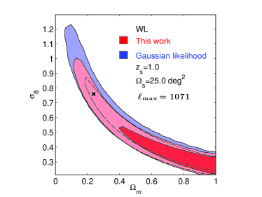
Figure 1 shows 1$\displaystyle\sigma$ and 2$\displaystyle\sigma$ confidence level constraints on the $\displaystyle\Omega_{\rm m}$–$\displaystyle\sigma_{8}$ plane. Note that $\displaystyle\Omega_{\rm m}$ denotes the present-day total matter density, i.e., the sum of the current dark matter and baryon densities. The red and blue contours show the marginalized constraints obtained by the copula likelihood (Eq. 4) and Gaussian likelihood (Eq. 5), respectively. Clearly the results from the copula likelihood (red contours) and Gaussian likelihood (blue contours) are significantly different. The contours obtained with the copula likelihood are shifted toward a parameter region that gives a lower convergence power compared to that from the Gaussian likelihood. This result is attributed to the fact that the median of the $\displaystyle\chi^{2}$ distribution for the convergence power spectrum is smaller than that of the Gaussian distribution.

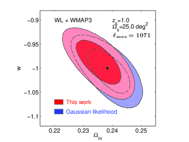
Figure 2 shows the constraints on the $\displaystyle\Omega_{\rm m}$–$\displaystyle w$ plane obtained when the weak lensing information is combined with data from WMAP3. Also in this case we see the difference between the results from the two likelihoods. Similarly, the contours obtained by the copula likelihood are shifted toward the parameter region that gives the lower power, i.e. smaller $\displaystyle\Omega_{\rm m}$ and larger $\displaystyle w$, than the Gaussian likelihood, as expected. Consequently, if one uses the (approximate) multivariate Gaussian likelihood, one will overestimate the lower bound and underestimate the upper one for the constraint on $\displaystyle w$. Specifically, we found an allowed range of the equation of state parameter $\displaystyle w$ for the Gaussian likelihood model as $\displaystyle-1.055<w<-0.956~{},$ while for the copula likelihood model as $\displaystyle-1.038<w<-0.941~{}$ at $\displaystyle 95$% confidence level. Therefore, a few percent of systematic error potentially exists in the parameter estimation if one uses approximate Gaussian likelihood.

Figure 1: Two-dimensional constraints (1$\displaystyle\sigma$ and 2$\displaystyle\sigma$ C.L.) on $\displaystyle\Omega_{\rm m}$ and $\displaystyle\sigma_{8}$ for survey area $\displaystyle\Omega_{\rm s}=25{\rm deg}^{2}$. The red and blue contours show the constraints obtained by likelihood based on the copula likelihood (Eq. 4) and Gaussian likelihood (Eq. 5), respectively. The cross symbol shows the fiducial cosmological parameters.

Figure 2: Same as Fig. 1, but two-dimensional marginalized constraints on $\displaystyle\Omega_{\rm m}$ and $\displaystyle w$ for weak lensing plus WMAP 3-yr results.

Impact on future weak lensing surveys. Next let us assume a survey area of 2000 deg², which roughly corresponds to the planned Subaru Weak Lensing Survey (Miyazaki et al., 2006). Because our ray-tracing simulation is limited to 25 deg², we have to extend it to estimate the mean power spectrum $\displaystyle\mu_{i}$ and their covariance with help from analytic treatments. When estimating the mean power spectrum $\displaystyle\mu_{i}$, we use the linear perturbation theory based on WMAP 3-yr fiducial cosmology for multipoles in the range $\displaystyle 8\leq\ell<\ell_{f}=72$, where $\displaystyle\ell_{f}$ corresponds to the largest angular mode of our ray-tracing simulation (5$\displaystyle\times$ 5 deg² for an area). For the covariance matrix $\displaystyle{\rm Cov}$, we assume that it has only diagonal elements for multipoles smaller than $\displaystyle\ell_{f}=72$ because the linear approximation is valid for that multipole range. In the absence of shape noise, the diagonal elements would arise from sample variance and should be equal to the power spectrum squared divided by the number of independent modes in the bin. Also, we assume that the covariances between the scales larger than $\displaystyle\ell_{f}=72$ and scales smaller than $\displaystyle\ell_{f}=72$ are zero, which means that the powers at the largest scales are independent from those at smaller scales.

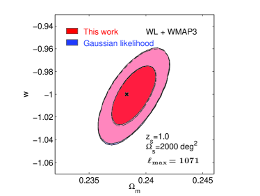
Figure 3 shows the constraints on the ($\displaystyle\Omega_{\rm m}$, $\displaystyle w$) plane obtained when weak lensing information with the survey area of $\displaystyle 2000$ deg² is combined with WMAP3. In this case, we do not see any significant difference between the results from the two likelihoods. This result is understood as follows. If one considers the larger survey area, $\displaystyle\Upsilon$ becomes larger at a fixed multipole because $\displaystyle\sigma^{2}$ becomes smaller (see, Eq. 7). Hence, $\displaystyle\chi^{2}$ distribution for the convergence power spectrum becomes well approximated by the Gaussian distribution at the fixed multipole. Even though at the lowest multipole bin the distribution may be deviated from Gaussian, the bulk of information comes from the large multipole bins, where the distribution is almost Gaussian. Hence the contours become indistinguishable.

It should be noted, however, that the Gaussianity in the distribution of the power spectrum should be due to our sparse binning of the multipole space. To utilize the information as much as possible, we have to divide the multipole space into a larger number of bins than we have done in this study. In such a case, the distribution of the power spectrum at each multipole bin will deviate from the Gaussian distribution and the copula likelihood will still be useful to model the probability of the power spectrum distribution.

Figure 3: Same as Fig. 2, but assumed survey area is 2000 deg² for weak lensing. This good agreement may not be caused by a physical reason, but rather attributed to the coarse binning.

Summary. In this Letter we constructed a likelihood function for the convergence power spectrum from weak lensing survey using copula. The copula likelihood function describes more accurately the distribution of the power spectrum derived from ray-tracing simulations and thus utilizes more information than the previous methods in the literature. We then used the copula likelihood model to calculate the allowed range of the cosmological parameters paying particular attention to the dark energy equation of state parameter $\displaystyle w$, and compare it with that derived from the conventional multivariate Gaussian likelihood model. We found that, for the $\displaystyle 25$ deg² weak lensing survey, the results can be different even combined with the CMB data, depending on which likelihood function is used. The difference is as large as a few percent.

For the $\displaystyle 2000$ deg² weak lensing survey, we found the results coincide with each other. This result allows us to use a multivariate Gaussian likelihood model for the future weak lensing survey, which will greatly simplify the parameter estimation analysis. We note, however, that this coincidence might be an artifact from our sparse binning of the multipole space. A full analysis with finer binning is difficult at present because computational cost is high, and we leave it for a future study.

Acknowledgments. We thank Agnieszka Pollo and Masahiro Takada for comments. We also thank the anonymous referees for careful reading of our manuscript and very useful and constructive suggestions that help to clarify our paper further. M.S. is supported by the JSPS. T.T.T. has been supported by Program for Improvement of Research Environment for Young Researchers from Special Coordination Funds for Promoting Science and Technology. This work is partially supported by the Grant-in-Aid for the Scientific Research Fund No. 20740105 (T.T.T,), No. 21740177, No. 22012004 (K.I.), and Grant-in-Aid for Scientific Research on Priority Areas No. 467 “Probing the Dark Energy through an Extremely Wide and Deep Survey with Subaru Telescope” commissioned by the MEXT of Japan.

References

- Miyazaki et al. (2006) S. Miyazaki, Y. Komiyama, H. Nakaya, Y. Doi, H. Furusawa, P. Gillingham, Y. Kamata, K. Takeshi, and K. Nariai, Proc. SPIE 6269, 9 (2006).
- Refregier et al. (2010) A. Refregier, A. Amara, T. D. Kitching, A. Rassat, R. Scaramella, J. Weller, and f. t. Euclid Imaging Consortium, arXiv:1001.0061 (2010).
- Hamana et al. (2003) T. Hamana, S. Miyazaki, K. Shimasaku, H. Furusawa, M. Doi, M. Hamabe, K. Imi, M. Kimura, Y. Komiyama, F. Nakata, et al., ApJ 597, 98 (2003).
- Jarvis et al. (2006) M. Jarvis, B. Jain, G. Bernstein, and D. Dolney, ApJ 644, 71 (2006).
- Semboloni et al. (2006) E. Semboloni, Y. Mellier, L. van Waerbeke, H. Hoekstra, I. Tereno, K. Benabed, S. D. J. Gwyn, L. Fu, M. J. Hudson, R. Maoli, et al., A&A 452, 51 (2006).
- Fu et al. (2008) L. Fu, E. Semboloni, H. Hoekstra, M. Kilbinger, L. van Waerbeke, I. Tereno, Y. Mellier, C. Heymans, J. Coupon, K. Benabed, et al., A&A 479, 9 (2008).
- Schrabback et al. (2010) T. Schrabback, J. Hartlap, B. Joachimi, M. Kilbinger, P. Simon, K. Benabed, M. Bradač, T. Eifler, T. Erben, C. D. Fassnacht, et al., A&A 516, A63+ (2010).
- Semboloni et al. (2010) E. Semboloni, T. Schrabback, L. van Waerbeke, S. Vafaei, J. Hartlap, and S. Hilbert, MNRAS pp. 1452–+ (2010).
- Sato et al. (2009) M. Sato, T. Hamana, R. Takahashi, M. Takada, N. Yoshida, T. Matsubara, and N. Sugiyama, ApJ 701, 945 (2009).
- Hartlap et al. (2009) J. Hartlap, T. Schrabback, P. Simon, and P. Schneider, A&A 504, 689 (2009).
- Ichiki et al. (2009) K. Ichiki, M. Takada, and T. Takahashi, Phys.Rev.D 79, 023520 (2009).
- Sato et al. (2010a) M. Sato, K. Ichiki, and T. T. Takeuchi, arXiv:1011.4997, Phys.Rev.D in press (2010a).
- Spergel et al. (2007) D. N. Spergel, R. Bean, O. Doré, M. R. Nolta, C. L. Bennett, J. Dunkley, G. Hinshaw, N. Jarosik, E. Komatsu, L. Page, et al., ApJS 170, 377 (2007).
- Sato et al. (2010b) M. Sato, M. Takada, T. Hamana, and T. Matsubara, arXiv:1009.2558 (2010b).
- Sklar (1959) A. Sklar, Publ. Inst. Statist. Univ. Paris 8, 1 (1959).
- Nelsen (2006) R. B. Nelsen, An Introduction to Copulas, 2nd edn (Springer, New York, 2006).
- Scherrer et al. (2010) R. J. Scherrer, A. A. Berlind, Q. Mao, and C. K. McBride, ApJ 708, L9 (2010).
- Takeuchi (2010) T. T. Takeuchi, MNRAS 406, 1830 (2010).
- Smith et al. (2003) R. E. Smith, J. A. Peacock, A. Jenkins, S. D. M. White, C. S. Frenk, F. R. Pearce, P. A. Thomas, G. Efstathiou, and H. M. P. Couchman, MNRAS 341, 1311 (2003).
- Takada and Jain (2009) M. Takada and B. Jain, MNRAS 395, 2065 (2009).
- Takahashi et al. (2009) R. Takahashi, N. Yoshida, M. Takada, T. Matsubara, N. Sugiyama, I. Kayo, A. J. Nishizawa, T. Nishimichi, S. Saito, and A. Taruya, ApJ 700, 479 (2009).
- Lewis and Bridle (2002) A. Lewis and S. Bridle, Phys.Rev.D 66, 103511 (2002).
- Gelman and Rubin (1992) A. Gelman and D. B. Rubin, Statistical Science 7, 457 (1992).