Can IBEX Identify Variations in the Galactic Environment of the Sun using Energetic Neutral Atom (ENAs)?

Abstract

The Interstellar Boundary Explorer (IBEX) spacecraft is providing the first all-sky maps of the energetic neutral atoms (ENAs) produced by charge-exchange between interstellar neutral H^o atoms and heliospheric solar wind and pickup ions in the heliosphere boundary regions. The ’edge’ of the interstellar cloud presently surrounding the heliosphere extends less than 0.1 pc in the upwind direction, terminating at an unknown distance, indicating that the outer boundary conditions of the heliosphere could change during the lifetime of the IBEX satellite. Using reasonable values for future outer heliosphere boundary conditions, ENA fluxes are predicted for one possible source of ENAs coming from outside of the heliopause. The ENA production simulations use three-dimensional MHD plasma models of the heliosphere that include a kinetic description of neutrals and a Lorentzian distribution for ions. Based on this ENA production model, it is then shown that the sensitivities of the IBEX 1.1 keV skymaps are sufficient to detect the variations in ENA fluxes that are expected to accompany the solar transition into the next upwind cloud. Approximately 20% of the IBEX 1.1 keV pixels appear capable of detecting the predicted model differences at the $3\sigma$ level, with these pixels concentrated in the Ribbon region. Regardless of the detailed ENA production model, the success of the modeled ${\bf B}\cdot{\bf R}\sim 0$ directions in reproducing the Ribbon locus, together with our results, indicate that the Ribbon phenomenon traces the variations in the heliosphere distortion caused by the relative pressures of the interstellar magnetic and gaseous components.

1 Introduction

The dynamic heliosphere varies with the properties of the surrounding interstellar cloud and the solar wind. A theoretical study of the expected heliosphere response to different types of interstellar clouds show that both the overall dimensions and hydrogen filtration should vary substantially with variations in the physical properties of circumheliospheric interstellar material (Müller et al., 2006, 2008). The presence of an interstellar magnetic field causes heliosphere asymmetries that can diagnose the properties of the surrounding interstellar material, but which are partially offset by the charge-exchange coupling of interstellar H^o and protons upstream of the heliopause (Pogorelov et al., 2009c; Opher et al., 2009; Ratkiewicz et al., 2008; Izmodenov, 2009). The velocity discontinuity observed between interstellar gas inside of the heliosphere (e.g. Witte, 2004) and interstellar material (ISM) towards the nearest stars in the upwind direction (36 Oph and $\alpha$ Cen, Landsman et al., 1984; Lallement et al., 1995; Wood et al., 2000; Linsky & Wood, 1996) is usually interpreted to indicate that the Sun is immersed in one interstellar cloud today, but will enter a separate cloud sometime in the next $\sim 4000$ years. The Interstellar Boundary Explorer (IBEX) is for the first time mapping heliospheric energetic neutral atoms, formed by charge-exchange between solar wind ions and pickup ions with neutral interstellar atoms (McComas et al., 2009b, a; Funsten et al., 2009b; Fuselier et al., 2009; Schwadron et al., 2009). In this paper we show that, depending on the source of ENAs observed, IBEX is capable of detecting the variable heliosphere boundary conditions that might accompany the expected (someday, it could be soon) solar transition into a new interstellar environment in the upwind direction.

The discovery of an unexpected ’Ribbon’ of ENA emission, in directions where the interstellar magnetic field draping over the heliosphere is thought to be perpendicular to the sightline, showed that IBEX may be detecting plasma-neutral interactions beyond the heliopause. The similar spectra of ENAs in the Ribbon and adjacent sightlines suggest that the Ribbon represents a selection effect rather than an ENA population with an fully independent origin. McComas et al. (2009a) and Schwadron et al. (2009) noted that the ribbon is organized by the most likely direction of the external interstellar magnetic field (ISMF), and proposed several different potential sources of the Ribbon including the possibility that the Ribbon might be created from a population of anisotropic suprathermal ions gyrating around the interstellar magnetic field just outside the heliopause. These ions could be indigenous to the outer heliosheath (beyond the heliopause) or more likely would arise from ENAs that propagated out from the supersonic solar wind and/or inner heliosheath (between the termination shock and the heliopause); these authors noted that the problem with this idea is that the relatively confined pitch angle distributions would need to be maintained long enough to create ”secondary ENAs”, which likely takes several years on average. Subsequently, Heerikhuisen et al. (2010) incorporated this idea, where outward propagating ENAs create an anisotropic population of pickup ions (PUI) in the outer heliosheath that seed ”secondary ENA” production several hundred AU upwind of the heliopause, into a quantitative model. While it is still uncertain how long the ion ring beam takes to scatter into a shell distribution (Florinski, Zank, Heerikhuisen, Hu and Khazanov, submitted), with marginally stable ring distributions predicted by some models for the distribution of the pitch angles of pickup ions in the outer heliosheath (Gamayhunov, Zhang, Rassoul, submitted to ApJ), the Heerikhuisen et al. simulation assumes that the re-neutralization time is essentially instantaneous compared to the scattering time so that the new secondary ENA will have a preferred direction that is perpendicular to the local ISMF direction. In this model, IBEX then sees these secondary ENAs where the gyration plane of the ion is aligned with the sightline to IBEX, i.e. where the sightline is perpendicular to the ISMF direction.

IBEX data are uniquely qualified to simultaneously test both the direction of the ISMF at the heliosphere and the density of interstellar neutrals. The ISMF drapes around the heliosphere, rotating by $\sim 30^{\circ}$ between ’infinity’ and the heliopause near the nose. The Ribbon is $\sim 20^{\circ}$ wide and at least $270^{\circ}$ long, possibly forming a complete circle in the sky. IBEX only sees ENAs with momentum vectors directed back towards the inner heliosphere. The long mean free paths of ENAs, e.g. $\sim 200$ AU for 1.1 keV ENAs in $n\mathrm{(p^{+})}$$\sim 0.1$ cm^-3 plasma, allow detection in the inner heliosphere of secondary ENAs formed in regions beyond the heliopause with elevated interstellar densities and relatively isotropic ENA velocities (compared to the outwards radial flows for primary ENAs produced in the supersonic solar wind, although not compared to the inner heliosheath ion populations). The solar wind contributing to ENA production includes both core ions from the expanding solar corona, and pickup ions formed inside of the heliosphere by charge exchange between interstellar neutrals and the core solar wind.

The predictive capabilities of global heliosphere models have improved significantly to accommodate observational constraints placed by the 10 AU difference in the termination shock distances found by the Voyager 1 and Voyager 2 spacecraft (Stone, 2007; Opher et al., 2009), the $\sim 5^{\circ}$ offset between the upwind directions of interstellar H^o and He^o flowing into the heliosphere determined from SOHO/SWAN and Ulysses/GAS data (Lallement et al., 2005; Witte, 2004; Frisch, 2008, where the He^o upwind direction must first be converted to J2000 coordinates for this comparison), the properties of the ISM surrounding the heliosphere (Slavin & Frisch, 2008), and now the IBEX data on ENA fluxes and the Ribbon. Although the IBEX Ribbon itself was not predicted by models of ENA formation in the heliosphere, the global heliosphere models provided the ISMF orientation that matches well with the configuration of the Ribbon in the sky (Schwadron et al., 2009; Pogorelov et al., 2009c).

In the discussions below we rely on the ENA production models quantified by Heerikhuisen et al. (2010); Pogorelov et al. (2009b) to predict the ENA fluxes for a heliosphere immersed in the next interstellar cloud versus the present-day surrounding interstellar cloud. The ENA production simulations use three-dimensional MHD plasma models of the heliosphere that include a kinetic description of neutrals and a Lorentzian distribution for solar wind protons to approximate the suprathermal population of pick-up ions in the heliosheath region. The interstellar neutrals, that are coupled self-consistently to the plasma component in the MHD heliosphere models, act to symmetrize the heliosphere. Any asymmetry in the quiescent plasma distribution (e.g. created by ISMF) results in variations in the number of charge-exchange events, creating new ions that are decelerated by the heliopause and therefore that mitigate the asymmetry (Pogorelov et al., 2008a, 2009c, 2009b). The LISM flow, for the assumed ISMF strength, is subfast magnetosonic (Table 1). This results in the absence of a bow shock in front of the heliopause, and increases the width of the region where the ISMF deviates from its unperturbed orientation. Since the local ISMF direction varies as interstellar protons approach the heliopause, the mean-free-path for the charge exchange interaction must also be included self-consistently in any Ribbon production models.

The Ribbon ENAs are formed upwind of the heliopause in the Heerikhuisen et al. (2010) model, so the outer boundary conditions set by the ISM have a direct impact on predicted ENA fluxes and provide a means of estimating ENA variations from a cloud transition, regardless of whether the model is correct in detail. Any model that reproduces the observed ${\bf B}\cdot{\bf R}\sim 0$ of the Ribbon, which is seen where the ISMF (${\bf B}$) is perpendicular to the sightline (${\bf R}$), should provide useful insights into the deformation of the heliosphere due to altered boundary conditions from the variable interstellar wind. Our conclusions here rely explicitly on the assumption that the Heerikhuisen et al. (2010) model provides a viable description of ENA production, both for the cloud we are in today and for the nearby cloud observed towards $\alpha$ Cen and 36 Oph in the upwind direction.

We focus on the 1.1 keV data, because the contrast between Ribbon ENA fluxes and diffuse ENA fluxes is stronger at this energy, and partly because of the enhanced outwards flow of ENAs from core solar wind ions that have typical energies near 1 keV. The ENA spectra are explicitly predicted by the heliosphere models, however this spectral information is not used here. The observed fluxes of $\sim 4.5$ keV ENAs are an order of magnitude lower than the 1.1 keV fluxes and the mean-free-paths are $\sim 50$% larger. Since the outflowing ion fluxes will decrease as $\sim R^{-2}$ with distance from the Sun $R$, both parent ion densities and the resulting 1-AU ENA densities are lower when production regions are further from the Sun.

2 Properties of the Upwind ISM

The boundary conditions of the heliosphere are set by the ISM, and vary over geologically short time-scales. Interstellar clouds within $\sim 50$ pc flow past the Sun with heliocentric velocities that cluster around $\sim 28$ km s^-1 (after projection effects are removed), or $\sim 1$ parsec per 35,000 yrs (Frisch & Slavin, 2006). If nearby ISM is in pressure equilibrium, then models of the interstellar cloud around the heliosphere (Slavin & Frisch, 2008) combined with ISM data (Redfield & Linsky, 2004) yield an estimate for the typical cloud length of $\sim 1$ pc. Cloud column densities for 23 cloud components towards stars within 10 pc yield a range of cloud lengths 0.06–3 pc, giving typical cloud crossing times for the Sun of $\sim 1,450-2.8\times 10^{5}$ years..

The velocity of the ISM at the heliosphere, which we term here the heliospheric ISM but which is also known as either the Local Interstellar Cloud (LIC) or the circumheliospheric ISM, is best set by the velocity of interstellar He^o observed inside of the heliosphere by the Ulysses satellite (Witte, 2004). Interstellar He^o experiences minimal filtration in the heliosheath regions ($<2$%, Müller & Zank, 2004) and is not subject to radiation pressure, so that variation in the interstellar He^o velocity as it traverses the heliosphere is minimal. The first comparisons between the velocities of interstellar gas in the heliosphere and outside of the heliosphere, towards stars in the upwind direction, showed differences of over 3 km s^-1 (Adams & Frisch, 1977). When the 26.3 km s^-1 He^o velocity is projected towards the nearest star in the upwind direction $\alpha$ CMa, 1.3 pc away and 50^∘ from the heliosphere nose, the projected heliospheric ISM velocity is –17.0 km s^-1, in contrast to the observed cloud velocity from the unsaturated Fe⁺ and Mg⁺ lines of $-18.0\pm 0.2$ km s^-1 (Linsky & Wood, 1996). The heliosphere nose direction is given by the upwind direction of He^o flowing through the heliosphere, or $\lambda,\beta=255.4^{\circ}\pm 0.5^{\circ},+5.1\pm 0.2^{\circ}$ (epoch J2000, Witte, 2004, and private communication). The star 36 Oph is 6 pc away and 10^∘ from the heliospheric nose. The projected heliospheric ISM velocity in this direction is –25.9 km s^-1, versus the observed cloud velocity from the Fe⁺ and Mg⁺ lines of $-28.1\pm 0.2$ km s^-1 (Wood et al., 2000). The limit on a cloud component at the heliospheric ISM velocity towards 36 Oph is $\sim 6\times 10^{16}$ cm^-2, giving an upper limit to the heliospheric ISM edge in this direction of 0.1 pc which will be traversed in less than 4000 years.

The interstellar cloud observed towards 36 Oph and $\alpha$ Oph is known as the G-cloud (Lallement & Bertin, 1992; Frisch et al., 2002; Redfield & Linsky, 2008), since it is close to the Sun in the galactic hemisphere. Although other possible clouds have been suggested as the next cloud to be encountered by the heliosphere (Frisch, 2003), the G-cloud remains the most likely future heliospheric environment.

The scenario examined here assumes that the Sun transitions directly from the heliospheric ISM to the G-cloud seen towards 36 Oph and $\alpha$ Cen. We determine the properties of the next cloud by assuming that the thermal and magnetic pressures in the heliospheric ISM are equal, and that the heliospheric ISM and G-clouds are in pressure equilibrium. The G-cloud temperature is found from the mass-dependent Doppler broadened widths of interstellar absorption lines, and is $5400\pm 500$ K towards $\alpha$ Cen, and $5900\pm 500$ towards 36 Oph (where the cloud column density is also larger by 70%). The cooler G-cloud temperatures are thus compensated by neutral densities that are 20% larger than the heliospheric ISM. The 9% higher velocity of the G-cloud, in comparison to the velocity of the ISM now surrounding the Sun, will increase the interstellar ram pressure even if thermal pressure and ionization levels remain constant. We test the sensitivity of ENA emission to the ISMF direction using two separate ISMF directions for the G-cloud. The first assumption is that the directions of the ISMF in the heliospheric ISM and G-clouds are the same (Models 2 and 3 in Table 1). For Model 4 we make an arbitrary assumption for the G-cloud ISMF direction, which is $28^{\circ}$ different from today’s field but less than the $\sim 30^{\circ}$ rotation of the ISMF between the ISM and the heliopause for the upwind direction. The detailed heliosphere boundary conditions used here for the next-cloud are listed in Table 1. We show below that the IBEX Ribbon is highly sensitive to even small variations in the ISMF direction, even when increased H^o densities mitigate the influence of the ISMF on heliospheric asymmetries.

3 ENA fluxes from encounter with Next Interstellar Cloud

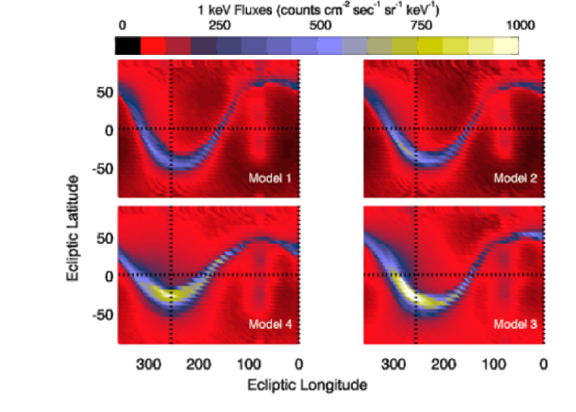
Figure 1: Four models of ENA fluxes at 1.1 keV, based on different values for the ISM that constrains the heliosphere (see Table 1). Model 1 is the initial model used to evaluate the IBEX results (Schwadron et al., 2009). Model 2 is the assumed benchmark model for the production of ENAs observed by IBEX today (Heerikhuisen et al. 2010). Models 3 and 4 utilize the same model, but with different heliosphere boundary conditions appropriate for the next upwind cloud. Model 3 represents 1.1 keV ENAs for a heliosphere constrained by the physical parameters of the next cloud in the upwind direction, where it is assumed that cloud is in pressure equilibrium with the circumheliospheric gas. The same ISMF direction of $\lambda,\beta=224^{\circ},41^{\circ}$ is assumed for Models 2 and 3. Model 4 is the same as Model 3, except that the direction of the ISMF differs by $28^{\circ}$, and is directed towards $\lambda,\beta=252^{\circ},42^{\circ}$. The dashed lines, in this and subsequent figures, intersect at the longitude of the heliosphere nose ($\lambda=255.4^{\circ}$) and the ecliptic plane.

The heliosphere model has been run for the interstellar boundary conditions listed for Models 1-4 in Table 1. The 1.1 keV ENA fluxes predicted by the resulting models are displayed in Fig. 1. Model 1 corresponds to the heliosphere model displayed in Schwadron et al. (2009). Model 2 (from Heerikhuisen et al., 2010) is the updated model we use for the heliosphere today. Models 3 and 4 correspond to the anticipated heliosphere environment in the next interstellar cloud, with Model 3 having a similar ISMF configuration as Model 2, and Model 4 showing a ISMF field with a different direction. The increased H^o density in Model 3 produces a brighter ribbon, while the ram and thermal pressures slightly increase and the magnetic pressure slightly decreases. The magnetic field in Model 2 plays a bigger role in deforming the heliosphere than in Model 3. Model 4 has the Ribbon shifted significantly because of the different ISMF direction.

The differences between the predicted ENA fluxes for Model 2 (the ’today-cloud’) and Model 3 (the G-cloud assuming the same ISMF direction as today-cloud) are directly displayed in Fig. 2. The ENA flux differences are obtained by subtracting the predicted fluxes of Model 2 ($F_{\mathrm{Mod2}}$) from the predicted fluxes of Model 3 ($F_{\mathrm{Mod3}}$, left). The most significant difference between the two models is the ram pressure of the neutrals, which is a factor of 1.8 larger for Model 3 versus Model 2. Over most of the sky, the higher flux of interstellar H^o into the heliosphere for Model 3 generates larger ENA fluxes, with the differences approaching the brightest observed fluxes. However the red pixels in Fig. 2, left, show regions where the today-cloud has higher fluxes than the next-cloud, and represent the small shift in the Ribbon position due to the increase in the ratio of thermal to magnetic pressures, $P_{\mathrm{ther}}$/$P_{\mathrm{mag}}$, in Model 3 compared to Model 2. The effect of increased H^o densities and thermal pressures are also seen in the increased ENA emissivity of the eastern flank of the heliosphere in the nose direction, where there is a bulge in total pressure (magnetic and thermal, see Fig. 1 in Heerikhuisen et al., 2010). Fig. 2, right, shows the flux differences between Model 2 and Model 4, where the ISMF direction in the G-cloud has been allowed to vary by 20^∘. This modest variation in the ISMF direction, while retaining the same field strength, leads to an obvious shift in the Ribbon location, and shows that variations in the direction of the ISMF draping over the heliosphere should be apparent in the ENA data.

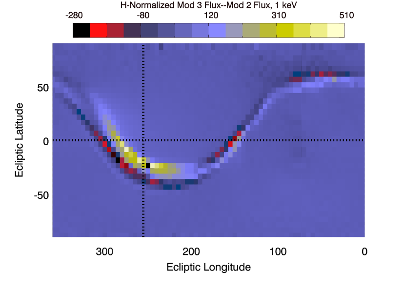
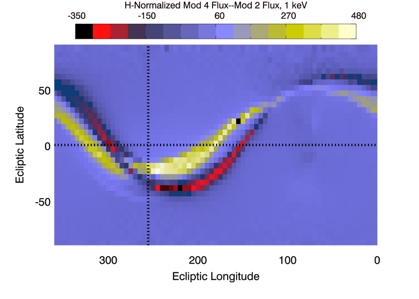
Figure 3: The differences between the ENA fluxes produced by the nominal G-cloud and the nominal present-day cloud, after normalizing the fluxes in Models 3 and 4 by the ratio of the neutral densities (0.65). Left: ($n$(H^∘)_Mod2/$n$(H^∘)_Mod3)*$F_{\mathrm{Mod3}}$– $F_{\mathrm{Mod2}}$. Right: ($n$(H^∘)_Mod2/$n$(H^∘)_Mod4)*$F_{\mathrm{Mod4}}$– $F_{\mathrm{Mod2}}$. Zero values of the difference (blue) along the ribbon imply that the ribbons in the two models overlay each other. The background blue regions, where difference counts are $\sim 0$, indicate the regions where ENA fluxes are linearly related to the neutral interstellar density in these models. Fluxes are given in the units of counts cm^-2 sec^-1 sr^-1 keV^-1.

The ENA-production model used here predicts that the ribbon and non-ribbon regions respond differently to variations in the interstellar density, because the ribbon also directly traces heliosphere asymmetries created by the ISMF. Fig. 3 shows the model differences modified by the ratio of $n\mathrm{(H^{\circ})}$ in Models 2 and 3 (0.65). The left figure shows 0.65 *$F_{\mathrm{Mod3}}$– $F_{\mathrm{Mod2}}$, and the right figure shows 0.65*$F_{\mathrm{Mod4}}$– $F_{\mathrm{Mod2}}$. The background blue regions, where difference counts are $\sim 0$, indicate regions where the ENA fluxes are linearly related to the neutral interstellar density. The variations in the ribbon colors show that the ribbon ENAs trace the distortion of the heliosphere, which depends on the asymmetries introduced by the relative interstellar, ram, and thermal pressures, and which changes with different ISM conditions.

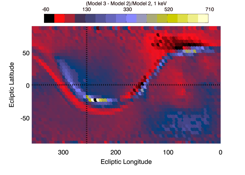
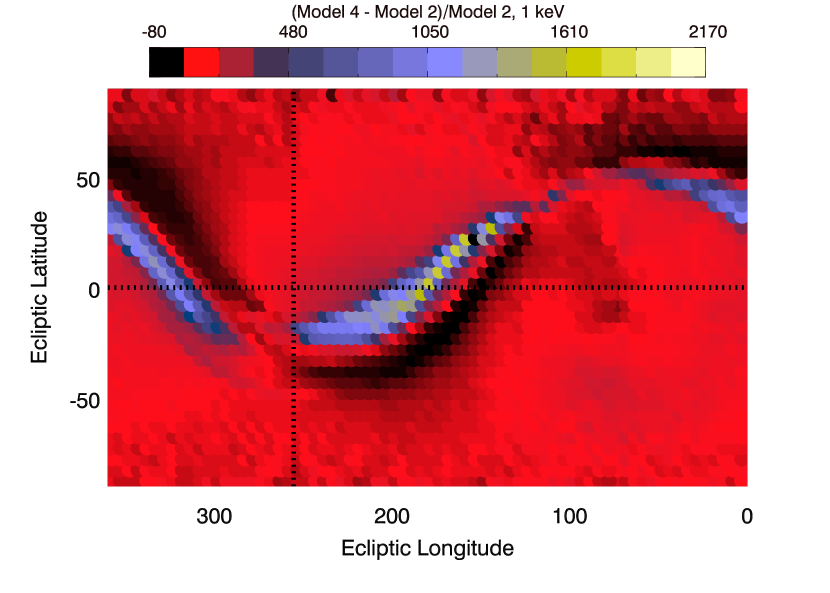
Figure 4: The percentage differences between the 1.1 keV ENA fluxes produced by the nominal G-cloud and the nominal present-day cloud. Left: 100($F_{\mathrm{Mod3}}$–$F_{\mathrm{Mod2}}$)/$F_{\mathrm{Mod2}}$. Right: 100($F_{\mathrm{Mod4}}$–$F_{\mathrm{Mod2}}$)/$F_{\mathrm{Mod2}}$. The right figure shows that the ribbon configuration is highly sensitive to any variation in the ISMF direction.

The differences in the ENA fluxes predicted by the two next-cloud models are quite obvious in the high-flux regions of the Ribbon, but less obvious (for this color scale) for the directions towards the tail. In order to emphasize the differences in the weaker diffuse ENA emission originating in the low-flux tail region, Fig. 4 shows the percentage differences between Models 3 and 2, ($F_{\mathrm{Mod3}}$–$F_{\mathrm{Mod2}}$)/$F_{\mathrm{Mod2}}$, and Models 4 and 2, ($F_{\mathrm{Mod4}}$–$F_{\mathrm{Mod2}}$)/$F_{\mathrm{Mod2}}$, with enhanced color scales. The percentage differences in the tail region for Model 3 are larger than for Model 4. The outer heliosheath region around the tail is the most disturbed part of the model results, since the flows are subsonic. Hence larger relative variations in ENA fluxes are possible.

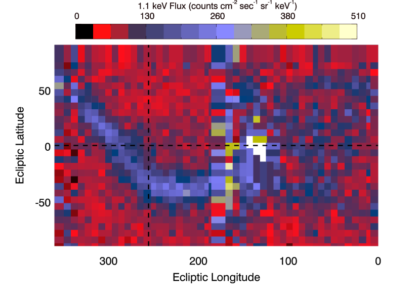
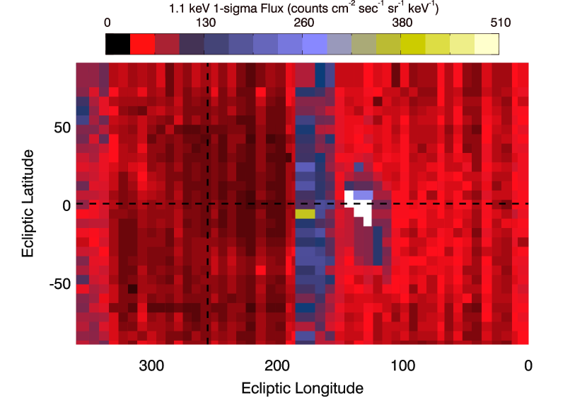
Figure 5: Left: The first 1.1 keV IBEX ENA skymap, corrected for the Compton-Getting effect (see text). Right: The $1\sigma$ statistical uncertainties on these data (see text).

The capability of IBEX to detect the ENA variations shown in Figs. 2–4 rests on the predicted differences in the modeled ENA fluxes compared to the flux uncertainties for the IBEX data. For this comparison, we use the first 1.1 keV ENA flux maps in the third energy passband (”ESA 3”) of the six energy passbands in the IBEX-HI neutral atom imager (Funsten et al., 2009a), where fluxes are an order of magnitude larger than at 4.5 keV (ESA 6). Fig. 5, left, shows ESA3 fluxes, after correction for the Compton-Getting (CG) shift in the energy and spatial distribution of high velocity particles due to the 30 km s^-1 orbital motion of the Earth (e.g. Gleeson & Axford, 1968). IBEX pixels are $\sim 7^{\circ}$. The CG corrections are based on a power-law energy spectra that are derived from adjacent energy passbands, typically $\sim E^{-1.6}$, which is evaluated over the look-direction and convolved with the energy response of the detector (see the Appendix in McComas et al., 2010, submitted to GRL, for details on the CG correction to the ENA energies measured by IBEX). The $1\sigma$ uncertainties ($dF_{\mathrm{1\sigma}}$) on these fluxes have been determined from the Poisson statistics propagated from the measurement uncertainties. The IBEX data are built from data processed by the IBEX Science Operations Center (ISOC) for the first all-sky IBEX map (orbits 11-34). The uncertainties in the ESA3 fluxes are shown in Fig. 5, right.

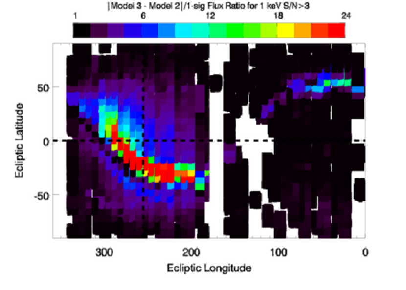
Figure 6: The differences between ENA fluxes predicted by models constrained by different boundary conditions, and compared to the $1\sigma$ measurement uncertainties in the ESA 3 energy passband (1.1 keV, see text). Left: The ratio of the absolute value of Model 3 minus Model 2 fluxes, to $1\sigma$ uncertainties ($|$$F_{\mathrm{Mod3}}$–$F_{\mathrm{Mod2}}$$|$)/$dF_{\mathrm{1\sigma}}$). Right: Same as left figure, but showing the absolute value of Model 4 minus Model 2 fluxes ($|$$F_{\mathrm{Mod4}}$–$F_{\mathrm{Mod2}}$$|$)/$dF_{\mathrm{1\sigma}}$). Pixels are left blank where fluxes are insignificant (S/N$<3$).

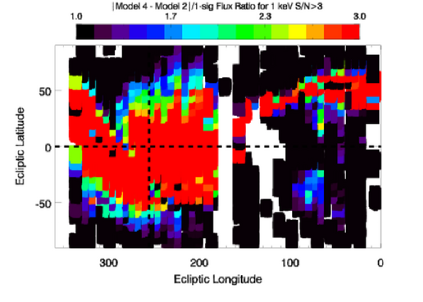
Figure 7: Same plot as Fig. 6, except that the color scale is coded to enhance the low flux areas in the tail region.

The measurement uncertainties for 1.1 keV fluxes can be compared to the predicted ENA flux differences for the next-cloud versus the present cloud, e.g. $|\Delta F_{\mathrm{model}}|$=$|$$F_{\mathrm{Mod3}}$–$F_{\mathrm{Mod2}}$$|$, based on the Heerikhuisen et al. (2010) model. For the comparison we preselect data points with signal-to-noise S/N$>3$. In Fig. 6, individual pixels in the Ribbon region for both models have values of $|\Delta F_{\mathrm{model}}|$/$dF_{\mathrm{1\sigma}}$$>>5$. The same difference map is plotted in Fig. 7, but now color-coded to enhance the differences in the tail region. Lower ENA fluxes towards the tail yield $|\Delta F_{\mathrm{model}}|$/$dF_{\mathrm{1\sigma}}$$\sim 1-2$ for individual pixels, which is somewhat larger for Model 3 than for Model 4. Groups of 25 pixels would yield a factor of 5 improvement in the S/N of the difference maps, while effectively smoothing the data over $\sim 125$ square-degrees, and still should provide a significant test. In order to use ENAs from the tail for identifying the next-cloud, either pixels in the tail must be grouped to improve statistics, or the comparison should wait for the better statistics of future skymaps.

The predicted ENA flux differences between the today-cloud and next cloud are testable with IBEX data. Twenty percent of the ESA 3 (1.1 keV) pixels with signal-to-noise S/N$>3$ test the flux differences between Model 3 and Model 2 at the $3\sigma$ level, or $|\Delta F_{\mathrm{model}}|$/$dF_{\mathrm{1\sigma}}$$>3$. In addition, 49% of the pixels test these flux differences at the $1\sigma$ level, with $|\Delta F_{\mathrm{model}}|$/$dF_{\mathrm{1\sigma}}$$>1$ (Fig. 8). Similar values are found for comparisons between the predicted flux differences between Model 4 and Model 2, where 18% of the pixels show model differences that are larger than the $3\sigma$ ESA3 flux uncertainties.

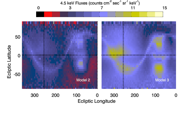
Figure 9: The predicted ENA fluxes at 4.5 keV (ESA 6 energy passband) are shown for Model 2 (left) and Model 3 (right).

We have also evaluated the variations in the 4.5 keV ENA fluxes for the environment of the next cloud (Fig. 9). Although the count rates in IBEX-HI ESA 6, at 4.5 keV, are lower by an order of magnitude than at 1.1 keV (Fig. 10, left), flux variations are predicted to occur when the effect of the increased interstellar density and velocity are included (Model 3 vrs. Model 2), as well as when the ISMF direction varies (Model 4 vrs. Model 2). For example, Model 2 has fluxes 5–6 counts cm^-2 sec^-1 sr^-1 keV^-1 at the locations $\lambda$,$\beta$=$253^{\circ},-33^{\circ}$ and $\lambda$,$\beta$=$268^{\circ},8^{\circ}$. For the same locations, Model 3 has fluxes a factor of $\sim 2$ higher. Further study of the energy spectrum of heliosheath ions is in progress, however, since the relatively large tail brightness predicted at 4.5 keV by Model 2 is difficult to distinguish in the data.

4 Discussion

If the Ribbon ENAs are produced as secondary ENAs beyond the heliopause as suggested by McComas et al. (2009) and Schwadron et al. (2009), and quantified by Heerikhuisen et al. (2010), then the position and intensity of the Ribbon provides a robust diagnostic of the interstellar magnetic field direction, neutral densities, and the cloud ram pressure at the heliosphere. Differences between the velocity of ISM inside of the heliosphere and towards the nearest stars in the upwind direction indicate that the Sun is near or at the edge of an interstellar cloud. Based on observations of the upwind ISM, and assuming that the upwind cloud is in pressure equilibrium with the heliospheric ISM, the next cloud is modeled with densities that are $\sim 50$% larger, and a heliocentric velocity 9% larger, than the cloud today. We predict the flux of ENAs from the next interstellar cloud to surround the heliosphere, and compare those predictions with the measurement uncertainties of the 1.1 keV ENA fluxes detected by IBEX in its first 6 month skymap. These results rely explicitly on the assumption that the Heerikhuisen et al. (2010) model is a viable description of ENA production both for the cloud we are in today and for the nearby cloud observed towards $\alpha$ Cen and 36 Oph in the upwind direction. Although our detailed conclusions rely on the accuracy of the Heerikhuisen et al. (2010) model, this study is a useful gedanken experiment that will help us understand the Ribbon sensitivity to variations in the properties of the ISM around the heliosphere.

The variations in ENA fluxes predicted for entry into the next cloud significantly exceed the measurement uncertainties for 20% of the ESA 3 pixels, which tend to be concentrated in the upwind hemisphere, and the variations are larger by a factor of two in some regions. The variations occur because the relative contributions of magnetic pressure and thermal ram pressure that deform the heliosphere are sensitive functions of the boundary conditions imposed by the ISM. If, in addition, the direction of the interstellar magnetic field shifts by as much as $28^{\circ}$, which is slightly larger than the Ribbon width, then significant differences in the ENA fluxes should be observed in individual pixels near the Ribbon. The heliosphere regions with very low ENA fluxes, such as the tail, provide a test of the cloud properties only if pixels are combined for better statistical significance before comparison with model predictions. The long term capability of IBEX to realistically detect such variations, which will also be superimposed on possible solar cycle variations, requires that the efficiencies in the IBEX sensors (conversion, scattering, sputtering in the conversion subsystem, secondary electron emission at the detector foils, microchannel plate efficiencies, for instance) either remain stable over years, or alternatively that the instrument performances are tightly monitored. IBEX-HI detector sensitivity is continuously monitored in a number of ways, such as comparison of coincident and non-coincident count rates (Funsten et al., 2005), and periodic gain tests.

Variations in the energy dependence and fluxes of ENAs will occur because of the variation of solar wind properties over the solar cycle. These solar cycle contributions fortunately can be modeled in detail using past and present data on the solar wind, and models of the heliosphere response to these variations. Every IBEX skymap is a historical map of the solar cycle because of the energy dependence of ENA travel times and cross sections (McComas et al. submitted, 2010), so that unraveling the solar cycle dependence will simultaneously constrain the ENA production models and improve future predictions of the ENA variations due to the next interstellar cloud.

In this discussion we considered the scenario where the next cloud is faster, slightly cooler, and more dense than the heliospheric ISM gas, as expected from pressure equilibrium and observational data. This study is a proof-of-concept, since the properties of the cloud edges are not established. The more extreme possibilities for the next galactic environment to be encountered by the Sun include a hot plasma without neutrals, and a cloud interface that is either evaporative or mixed with hot plasma by shear flows. If interstellar clouds within 10 pc are in pressure equilibrium, they will typically fill 20% of the sightline to the stars. The intervening voids evidently will be filled with the low density hot gas that creates the Local Bubble soft X-ray emission, although the emissivity of this plasma is somewhat uncertain because of solar wind contamination (Koutroumpa et al., 2008). Should the heliosphere enter the diffuse plasma attributed to the Local Bubble interior, both interstellar neutrals and exo-heliospheric ENAs will vanish. IBEX and other spacecraft will readily detect this condition. Another possibility for the next solar environment would be an evaporative interface that would form upwind between the heliospheric ISM and hot plasma. Such an interface will show steep increases in the cloud velocity and pressure, and decreases in density, over spatial scales that are determined by the angle between the ISMF and cloud surface (Slavin & Frisch, 2008).

The present study considers the ENA fluxes for two separate models of the circumheliospheric cloud, but ignores possible variations due to changes in the heliosphere configuration during the transitions between the two clouds. The predicted thickness of the conductive boundary on the cloud around the heliosphere, defined as where the temperature falls to 50% of the asymptotic temperature, is 0.32–0.34 pc for an ISMF direction that makes an angle of 30^o with the cloud surface (Slavin & Frisch, 2008, Models 26 and 27, also see Fig. 2, where the cloud edge starts at 3 pc). In the upwind direction the outflow speeds in the conductive boundary are 20–30 km s^-1, and opposite to the cloud motion, so that the Sun could traverse the conductive boundary in approximately $\sim 12,000$ years for these models. Based on the above models, we expect the change in heliosphere properties for such an environment to be clearly observable in the resulting ENA flux detected by IBEX. A turbulent mixing layer will also produce strong gradients in the temperature and ionization of the surrounding ISM (Slavin et al., 1993). The ENA emissions for a conductive boundary on the surrounding cloud are discussed in detail in Grzedzielski et al. (2010), where the Sun is estimated to emerge from the interface within $\sim 500$ years. An alternative possibility is that the G-cloud may be denser than has been assumed in this study. If the interstellar $\mathrm{N(Ca^{+}})$ absorption formed at the G-cloud velocity is entirely within a few parsecs of the Sun, then comparisons between the clouds in the $\alpha$ Cen and $\alpha$ Oph sightlines suggest a tiny cold cloud in addition to the warmer gas (Frisch, 2003).

The comparisons in this paper are made without consideration of the solar cycle, although the outer heliosheath regions respond to the variations in the solar wind dynamic pressure and magnetic field that characterize the solar activity cycle (Washimi & Tanaka, 1999; Scherer & Fahr, 2003; Zank & Müller, 2003; Pogorelov et al., 2009a). Although the solar cycle will cause the heliosphere to expand and contract as the solar wind dynamic pressure changes, these pulses travel only a relatively short distance upstream of the heliopause ($\sim 100$ AU). The influence of the solar cycle on ENA production and the Ribbon phenomenon is not yet understood. The Ribbon intensity may vary over latitudes due to the ion energy differences and travel times. The extremely low levels of solar activity during the first year of IBEX observations suggests the solar activity cycle variations must first be understood before reaching a conclusion that we have entered a new interstellar cloud (Pogorelov et al., 2008b; Sternal et al., 2008). As the theoretical models of ENA production become increasingly robust, we expect that studies such as this will yield definitive information on both the heliosphere boundary conditions and the physical properties of the interstellar cloud around the Sun. Finally, while this study has examined only one of the possible sources of the Ribbon currently under discussion, the other ideas for producing the ribbon (McComas et al., 2009a) also generally invoke and seek to match up with the orientation of the external IMF, so even if another explanation eventually becomes accepted, it may still be possible to directly detect the interstellar transition with IBEX.

Table 1: Properties of Circumheliospheric Interstellar Material used for Models

Quantity	LIC	Model 1	Model 2	Model 3	Model 4
		Original	Today	Next (same ISMF)	Next (new ISMF)
$n\mathrm{(H^{\circ})}$  (cm-3)	0.19	0.15	0.15	0.23	0.23
$n\mathrm{(p^{+})}$  (cm-3)	0.06	0.06	0.06	0.08	0.08
$V$  (km s-1)	–26.3	–26.4	–26.4	–28.8	–28.8
$T$  (K)	6300	6530	6530	5400	5400
$|$${B}$$|$ ($\mu$G)	[2.7]	3.	3.	2.8	2.8
${B}$ direction, $\lambda$,$\beta$		$237.^{\circ},30^{\circ}$	$224^{\circ},41^{\circ}$	$224^{\circ},41^{\circ}$	$252^{\circ},42^{\circ}$
${B}$ direction, $\ell$,$b$		$22.^{\circ},41^{\circ}$	$36^{\circ},53^{\circ}$	$36^{\circ},53^{\circ}$	$40.^{\circ},32^{\circ}$
Magnetosonic Mach	1.0	1.1	1.1	0.8	0.8
number

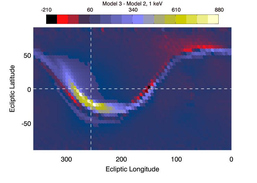
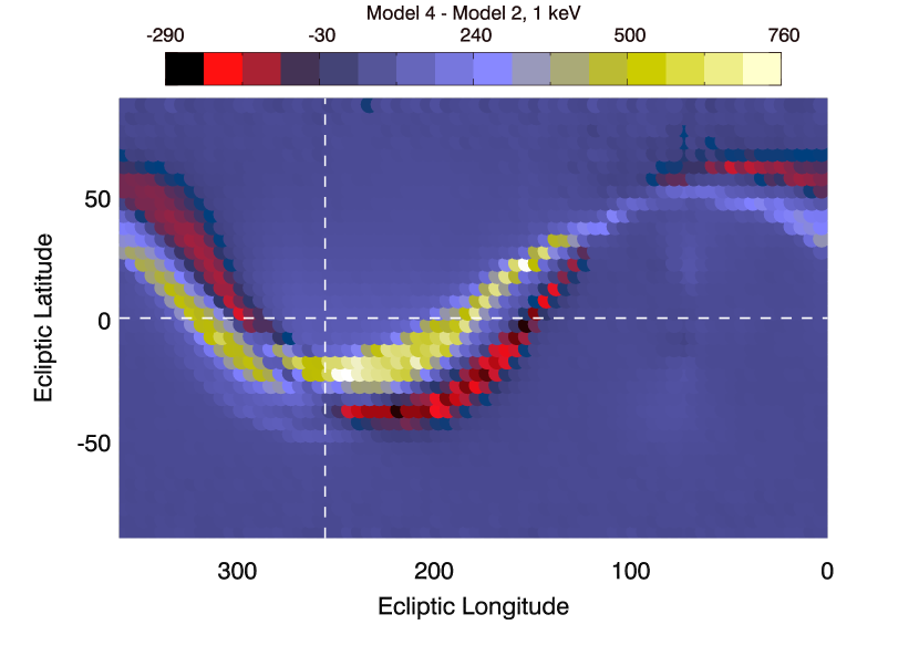
Figure 2: The differences between the ENA fluxes produced by the nominal G-cloud and the nominal LIC. Left: Model 3–Model 2 ($F_{\mathrm{Mod3}}$– $F_{\mathrm{Mod2}}$). Right: Model 4–Model 2 ($F_{\mathrm{Mod4}}$– $F_{\mathrm{Mod2}}$). The different distortions of the heliosphere caused by variations in the relative magnetic and thermal ram pressures of the ISM are apparent on the northeast flank of the heliopause in the left figure. The right figure shows that the ribbon configuration is highly sensitive to variations in the ISMF direction. The differences in the distortion of the heliosphere towards the tail region are marginally visible. Fluxes are given in the units of counts cm^-2 sec^-1 sr^-1 keV^-1.

Figure 8: The ESA 3 fluxes (ordinate) are compared to the significance of the model differences (abscissa) at each pixel on the sky for Models 3 and 2 (left) and Models 4 and 2 (right). The abscissa shows the differences in the fluxes of the two models, divided by the $1\sigma$ measurement uncertainties on the ESA 3 data. Only ”good” ESA 3 pixels with S/N$>3$ are plotted. The differences between Models 3 and 2 are tested at the $3\sigma$ level by 20% of all ESA 3 pixels, while 49% of all pixels test these differences at the $1\sigma$ level, for example.

Figure 10: The observed ESA 6 ENA fluxes at 4.5 keV are shown (left), together with the $1\sigma$ uncertainties on those fluxes (right).

References

- Adams & Frisch (1977) Adams, T. F. & Frisch, P. C. 1977, ApJ, 212, 300
- Frisch (2003) Frisch, P. C. 2003, ApJ, 593, 868
- Frisch (2008) —. 2008, ApJ accepted (arXiv:0804.1901v2)
- Frisch (2010) —. 2010, ApJ, 714, 1679
- Frisch et al. (2002) Frisch, P. C., Grodnicki, L., & Welty, D. E. 2002, ApJ, 574, 834
- Frisch & Slavin (2006) Frisch, P. C. & Slavin, J. D. 2006, Astrophysics and Space Sciences Transactions, 2, 53
- Funsten et al. (2009a) Funsten, H. O., Allegrini, F., Bochsler, P., Dunn, G., Ellis, S., Everett, D., Fagan, M. J., Fuselier, S. A., Granoff, M., Gruntman, M., Guthrie, A. A., Hanley, J., Harper, R. W., Heirtzler, D., Janzen, P., Kihara, K. H., King, B., Kucharek, H., Manzo, M. P., Maple, M., Mashburn, K., McComas, D. J., Moebius, E., Nolin, J., Piazza, D., Pope, S., Reisenfeld, D. B., Rodriguez, B., Roelof, E. C., Saul, L., Turco, S., Valek, P., Weidner, S., Wurz, P., & Zaffke, S. 2009a, Space Science Reviews, 146, 75
- Funsten et al. (2009b) Funsten, H. O., Allegrini, F., Crew, G. B., DeMajistre, R., Frisch, P. C., Fuselier, S. A., Gruntman, M., Janzen, P., McComas, D. J., Möbius, E., Randol, B., Reisenfeld, D. B., Roelof, E. C., & Schwadron, N. A. 2009b, Science, 326, 964
- Funsten et al. (2005) Funsten, H. O., Harper, R. W., & McComas, D. J. 2005, Review of Scientific Instruments, 76, 053301
- Fuselier et al. (2009) Fuselier, S. A., Allegrini, F., Funsten, H. O., Ghielmetti, A. G., Heirtzler, D., Kucharek, H., Lennartsson, O. W., McComas, D. J., Möbius, E., Moore, T. E., Petrinec, S. M., Saul, L. A., Scheer, J. A., Schwadron, N., & Wurz, P. 2009, Science, 326, 962
- Gleeson & Axford (1968) Gleeson, L. J. & Axford, W. I. 1968, Ap&SS, 2, 431
- Grzedzielski et al. (2010) Grzedzielski, S., Bzowski, M., Czechowski, A., Funsten, H. O., McComas, D. J., & Schwadron, N. A. 2010, ArXiv e-prints
- Heerikhuisen et al. (2010) Heerikhuisen, J., Pogorelov, N. V., Zank, G. P., Crew, G. B., Frisch, P. C., Funsten, H. O., Janzen, P. H., McComas, D. J., Reisenfeld, D. B., & Schwadron, N. A. 2010, ApJ, 708, L126
- Izmodenov (2009) Izmodenov, V. V. 2009, Space Science Reviews, 143, 139
- Koutroumpa et al. (2008) Koutroumpa, D., Lallement, R., Kharchenko, V., & Dalgarno, A. 2008, ArXiv e-prints, 805
- Lallement & Bertin (1992) Lallement, R. & Bertin, P. 1992, A&A, 266, 479
- Lallement et al. (1995) Lallement, R., Ferlet, R., Lagrange, A. M., Lemoine, M., & Vidal-Madjar, A. 1995, A&A, 304, 461
- Lallement et al. (2005) Lallement, R., Quémerais, E., Bertaux, J. L., Ferron, S., Koutroumpa, D., & Pellinen, R. 2005, Science, 307, 1447
- Landsman et al. (1984) Landsman, W. B., Henry, R. C., Moos, H. W., & Linsky, J. L. 1984, ApJ, 285, 801
- Linsky & Wood (1996) Linsky, J. L. & Wood, B. E. 1996, ApJ, 463, 254
- Müller & Zank (2004) Müller, H.-R. & Zank, G. P. 2004, J. Geophys. Res., 109, A07104, 7104
- McComas et al. (2009a) McComas, D. J., Allegrini, F., Bochsler, P., Bzowski, M., Christian, E. R., Crew, G. B., DeMajistre, R., Fahr, H., Fichtner, H., Frisch, P. C., Funsten, H. O., Fuselier, S. A., Gloeckler, G., Gruntman, M., Heerikhuisen, J., Izmodenov, V., Janzen, P., Knappenberger, P., Krimigis, S., Kucharek, H., Lee, M., Livadiotis, G., Livi, S., MacDowall, R. J., Mitchell, D., Möbius, E., Moore, T., Pogorelov, N. V., Reisenfeld, D., Roelof, E., Saul, L., Schwadron, N. A., Valek, P. W., Vanderspek, R., Wurz, P., & Zank, G. P. 2009a, Science, 326, 959
- McComas et al. (2009b) McComas, D. J., Allegrini, F., Bochsler, P., Bzowski, M., Collier, M., Fahr, H., Fichtner, H., Frisch, P., Funsten, H. O., Fuselier, S. A., Gloeckler, G., Gruntman, M., Izmodenov, V., Knappenberger, P., Lee, M., Livi, S., Mitchell, D., Möbius, E., Moore, T., Pope, S., Reisenfeld, D., Roelof, E., Scherrer, J., Schwadron, N., Tyler, R., Wieser, M., Witte, M., Wurz, P., & Zank, G. 2009b, Space Science Reviews, 146, 11
- Müller et al. (2008) Müller, H., Woodman, L. M., & Zank, G. P. 2008, in American Institute of Physics Conference Series, Vol. 1039, American Institute of Physics Conference Series, ed. G. Li, Q. Hu, O. Verkhoglyadova, G. P. Zank, R. P. Lin, & J. Luhmann , 384–389
- Müller et al. (2006) Müller, H.-R., Frisch, P. C., Florinski, V., & Zank, G. P. 2006, ApJ, 647, 1491
- Opher et al. (2009) Opher, M., Richardson, J. D., Toth, G., & Gombosi, T. I. 2009, Space Science Reviews, 143, 43
- Pogorelov et al. (2009a) Pogorelov, N. V., Borovikov, S. N., Zank, G. P., & Ogino, T. 2009a, ApJ, 696, 1478
- Pogorelov et al. (2009b) Pogorelov, N. V., Heerikhuisen, J., Mitchell, J. J., Cairns, I. H., & Zank, G. P. 2009b, ApJ, 695, L31
- Pogorelov et al. (2008a) Pogorelov, N. V., Heerikhuisen, J., & Zank, G. P. 2008a, ApJ, 675, L41
- Pogorelov et al. (2009c) Pogorelov, N. V., Heerikhuisen, J., Zank, G. P., & Borovikov, S. N. 2009c, Space Science Reviews, 143, 31
- Pogorelov et al. (2008b) Pogorelov, N. V., Zank, G. P., & Ogino, T. 2008b, Advances in Space Research, 41, 306
- Ratkiewicz et al. (2008) Ratkiewicz, R., Ben-Jaffel, L., & Grygorczuk, J. 2008, in Astronomical Society of the Pacific Conference Series, Vol. 385, Numerical Modeling of Space Plasma Flows, ed. N. V. Pogorelov, E. Audit, & G. P. Zank, 189–+
- Redfield & Linsky (2004) Redfield, S. & Linsky, J. L. 2004, ApJ, 613, 1004
- Redfield & Linsky (2008) —. 2008, ApJ, 673, 283
- Scherer & Fahr (2003) Scherer, K. & Fahr, H. J. 2003, Annales Geophysicae, 21, 1303
- Schwadron et al. (2009) Schwadron, N. A., Bzowski, M., Crew, G. B., Gruntman, M., Fahr, H., Fichtner, H., Frisch, P. C., Funsten, H. O., Fuselier, S., Heerikhuisen, J., Izmodenov, V., Kucharek, H., Lee, M., Livadiotis, G., McComas, D. J., Moebius, E., Moore, T., Mukherjee, J., Pogorelov, N. V., Prested, C., Reisenfeld, D., Roelof, E., & Zank, G. P. 2009, Science, 326, 966
- Slavin & Frisch (2008) Slavin, J. D. & Frisch, P. C. 2008, A&A, 491, 53
- Slavin et al. (1993) Slavin, J. D., Shull, J. M., & Begelman, M. C. 1993, ApJ, 407, 83
- Sternal et al. (2008) Sternal, O., Fichtner, H., & Scherer, K. 2008, A&A, 477, 365
- Stone (2007) Stone, E. C. 2007, AGU Fall Meeting Abstracts, A1+
- Washimi & Tanaka (1999) Washimi, H. & Tanaka, T. 1999, Advances in Space Research, 23, 551
- Witte (2004) Witte, M. 2004, A&A, 426, 835
- Wood et al. (2000) Wood, B. E., Linsky, J. L., & Zank, G. P. 2000, ApJ, 537, 304
- Zank & Müller (2003) Zank, G. P. & Müller, H. 2003, in American Institute of Physics Conference Series, Vol. 679, Solar Wind Ten, ed. M. Velli, R. Bruno, F. Malara, & B. Bucci, 762–765