Reverse Nearest Neighbors Search in High Dimensions
using Locality-Sensitive Hashing

Abstract

We investigate the problem of finding reverse nearest neighbors efficiently. Although provably good solutions exist for this problem in low or fixed dimensions, to this date the methods proposed in high dimensions are mostly heuristic. We introduce a method that is both provably correct and efficient in all dimensions, based on a reduction of the problem to one instance of $\varepsilon$-nearest neighbor search plus a controlled number of instances of exhaustive $r$-$\mathcal{PLEB}$, a variant of Point Location among Equal Balls where all the $r$-balls centered at the data points that contain the query point are sought for, not just one. The former problem has been extensively studied and elegantly solved in high dimensions using Locality-Sensitive Hashing (LSH) techniques. By contrast, the latter problem has a complexity that is still not fully understood. We revisit the analysis of the LSH scheme for exhaustive $r$-$\mathcal{PLEB}$ using a somewhat refined notion of locality-sensitive family of hash function, which brings out a meaningful output-sensitive term in the complexity of the problem. Our analysis, combined with a non-isometric lifting of the data, enables us to answer exhaustive $r$-$\mathcal{PLEB}$ queries (and down the road reverse nearest neighbors queries) efficiently. Along the way, we obtain a simple algorithm for answering exact nearest neighbor queries, whose complexity is parametrized by some condition number measuring the inherent difficulty of a given instance of the problem.

1 Introduction

Proximity queries are ubiquitous in science and engineering, and given their natural importance they have received a lot of attention from the computer science community [8, 10, 17, 29]. Nearest Neighbor ($\mathcal{NN}$) search is certainly among the most popular ones. Given a finite set $P$ with $n$ points sitting in some metric space $(X,\mathrm{d})$, the goal is to preprocess $P$ in such a way that, for any query point $q\in X$, a nearest neighbor of $q$ among the set $P\setminus\{q\}$ can be found quickly. The $\mathcal{NN}$ query can be easily answered in linear time by brute force search, so the algorithmic challenge is to preprocess the data points so as to find the answer in sub-linear time. Numerous methods have been proposed, however their performances degrade significantly when the dimensionality $d$ of the data increases — a phenomenon known as the curse of dimensionality. Typically, they suffer from either space or query time that is exponential in $d$ , and so they become no better than brute-force search when $d$ becomes higher than a few dozens or hundreds [34].

In light of the apparent hardness of $\mathcal{NN}$ search, an approximate version of the problem called $\varepsilon$-$\mathcal{NN}$ has been considered, where the answer can be any point of $P\setminus\{q\}$ whose distance to $q$ is within a given factor $(1+\varepsilon)$ of the true nearest neighbor distance [3, 7, 18, 22, 26]. Inspired from the random projection techniques developed by Kleinberg [22], Indyk and Motwani [18] and Kushilevitz et al. [26] proposed data structures to answer $\varepsilon$-$\mathcal{NN}$ queries with truly sublinear runtime and fully polynomial space complexity. The approach developped in [18] is based on the idea of Locality-Sensitive Hashing (LSH), which consists in hashing the data and query points into a collection of tables indexed by random hash functions, such that the query point $q$ has more chance to collide with nearby data points than with data points lying far away. This technique solves a decision version of the $\varepsilon$-$\mathcal{NN}$ problem called Point Location among Equal Balls ($(r,\varepsilon)$-$\mathcal{PLEB}$), which asks to decide whether the distance of $q$ to $P\setminus\{q\}$ is below a given threshold $r$ or above $r(1+\varepsilon)$. The output is proven correct with high probability, and the query time is bounded by $O(dn^{\varrho}\textup{polylog}\;n)$ for some constant $\varrho=\frac{1}{1+\Theta(\varepsilon)}$. Moreover, Indyk and Motwani [18] proposed a reduction of $\varepsilon$-$\mathcal{NN}$ search to a poly-logarithmic number of $(r,\varepsilon)$-$\mathcal{PLEB}$ queries, thus providing a fully sublinear-time and polynomial-space procedure for solving $\varepsilon$-$\mathcal{NN}$. Although originally designed for the Hamming cube, LSH was later extended [2, 11, 15] to affine spaces $\mathbb{R}^{d}$ equipped with $\ell_{s}$-norms, $s\in(0,2]$.

In this paper we mainly focus on the reverse problem, known as Reverse Nearest Neighbors ($\mathcal{RNN}$) search. Given a finite set $P$ with $n$ points sitting in some metric space $(X,d)$, the goal is to preprocess $P$ in such a way that, for any query point $q\in X$, one can find the influence set of $q$, i.e. the set $\mathcal{RNN}_{P}(q)$ formed by the points $p\in P\setminus\{q\}$ that are closer to $q$ than to $P\setminus\{p\}$. Such points are called reverse nearest neighbors of $q$. $\mathcal{RNN}$ queries arise in many different contexts, and it is no surprise that they have received a lot of attention since their formal introduction by Korn and Muthukrishnan [23]. A wealth of methods have been proposed [1, 4, 9, 12, 20, 23, 25, 30, 31, 32, 33], which behave well in practice on some classes of inputs. However, these methods are mostly heuristic, and to date very little is known about the theoretical complexity of $\mathcal{RNN}$ search, except in low [5, 27] or fixed [6] dimensions, where the dimensionality of the data can be considered as a mere constant. The crux of the matter is that, in contrast to ($\varepsilon$-)$\mathcal{NN}$ search, the answer to an $\mathcal{RNN}$ query is not a single point but a set of points, whose size can be up to exponential in the ambient dimension [28], so there is no way to achieve a systematic sub-linear query time. Ideally, one would like to achieve a query time of the form $\tilde{O}(n^{\varrho}+|\mathcal{RNN}_{P}(q)|)$, where $\varrho$ is a constant less than $1$ and $|\mathcal{RNN}_{P}(q)|$ is the size of the reverse nearest neighbors set. The big-$\tilde{O}$ notation may hide extra factors that are polynomial in $d$ and poly-logarithmic in $n$. Intuitively, the first term in the bound would represent the incompressible time needed to locate the query point $q$ with respect to the point cloud $P$, as in a standard $\mathcal{NN}$ query, while the second term would represent the size of the sought-for answer.

Our contributions.

Our main contribution (see Section 5) is a reduction of $\mathcal{RNN}$ search to one instance of $\varepsilon$-$\mathcal{NN}$ search plus a poly-logarithmic number of instances of exhaustive $r$-$\mathcal{PLEB}$, a set-theoretic version of $\mathcal{PLEB}$ where not only one $r$-ball containing the query point $q$ is sought for, but all such balls. Our reduction is based on a partitioning of the data points into buckets according to their nearest neighbor distances, combined with a pruning strategy that prevents the inspection of too many buckets at query time.

Turning our reduction into an effective algorithm for $\mathcal{RNN}$ search requires to adapt the LSH scheme to solve exhaustive $r$-$\mathcal{PLEB}$ queries. Such an adatptation was proposed in [29, Chapter 1], with expected query time $\tilde{O}(n^{\varrho}+n^{\varrho}|\mathcal{B}_{P}(q,r(1+\varepsilon))|)$, where $\varrho=\frac{1}{1+\Theta(\varepsilon)}$ and where $\varepsilon>0$ is a user-defined parameter. Even though the ouput of the query is the set $\mathcal{B}_{P}(q,r)$, the query time depends on the size of the superset $\mathcal{B}_{P}(q,r(1+\varepsilon))$, and when choosing $\varepsilon$ the user must find a trade-off between increasing the size of $\mathcal{B}_{P}(q,r(1+\varepsilon))$ and increasing the average retrieval cost $n^{\varrho}$ per point of $\mathcal{B}_{P}(q,r(1+\varepsilon))$. In Section 3 we revisit the analysis of [29, Chapter 1] using a somewhat finer concept of locality-sensitive hashing (see Definition 3.1), which enables us to quantify more precisely the amount of collisions with the query point that may occur within the hash tables stored in the LSH data structure. Taking advantage of this refined analysis, we propose a simple extra preprocessing step that reduces the average retrieval cost per point of $\mathcal{B}_{P}(q,r(1+\varepsilon))$ down to $n^{\alpha}$ for some constant $\alpha\leq\varepsilon\varrho<\varepsilon$, thereby making the previous trade-off no longer necessary. The price to pay is a slight degradation of the absolute term $n^{\varrho}$ in the complexity bound, which rises to $n^{\varrho^{\prime}}$ where $\varrho^{\prime}=\frac{1}{1+\Theta(\varepsilon^{2})}$ (Theorem 3.7). All in all, the query time bound becomes $\tilde{O}(n^{\varrho^{\prime}}+n^{\alpha}|\mathcal{B}_{P}(q,r(1+\varepsilon))|)$ and therefore remains sublinear in $n$ as long as $|\mathcal{B}_{P}(q,r(1+\varepsilon))|\leq n^{1-\varepsilon}$. Intuitively, our extra preprocessing step consists in lifting the point cloud $P$ and query point $q$ one dimension higher through some highly non-isometric embedding, so that the induced metric distortion moves $q$ away from $P$ and further concentrates the distribution of the distances to $q$ around the parameter value $r$, thereby reducing the total number of collisions with $q$ within the hash tables. The output of the query can still be proven correct thanks to the fact that the embedding preserves the order of the distances to $q$. This approach stands in contrast to the general trend of applying low-distortion embeddings to solve proximity queries.

Down the road, these advances lead to an algorithm for solving $\mathcal{RNN}$ queries with high probability in expected $\tilde{O}(\frac{1}{\varepsilon}n^{1/(1+\Theta(\varepsilon^{2}))}+n^{\varepsilon}|O(\varepsilon)\mbox{-}\mathcal{RNN}_{P}(q)|)$ time using fully polynomial space, where $\varepsilon>0$ is a user-defined parameter and $O(\varepsilon)\mbox{-}\mathcal{RNN}_{P}(q)$ is a superset of $\mathcal{RNN}_{P}(q)$ whose points are $O(\varepsilon)$-close to being true reverse nearest neighbors of $q$ (Theorem 5.3). To the best of our knowledge, this is the first algorithm for answering $\mathcal{RNN}$ queries that is provably correct and efficient in all dimensions. Furthermore, the algorithm and its analysis extend naturally to the bichromatic setting where the data points are split into two disjoint categories, e.g. clients and servers, a scenario that is encountered in various applications [23].

Along the way, in Section 4 we obtain a simple algorithm that can answer exact $\mathcal{NN}$ queries in expected $\tilde{O}(n^{1/(1+\Theta(\varepsilon^{2}))}+n^{\varepsilon}|O(\varepsilon)\mbox{-}\mathcal{NN}_{P}(q)|)$ time using fully polynomial space, where $\varepsilon>0$ is a user-defined parameter and $O(\varepsilon)\mbox{-}\mathcal{NN}_{P}(q)$ is a set of approximate nearest neighbors of $q$ (Theorem 4.3). The first term in the running time bound corresponds to a standard $\varepsilon$-$\mathcal{NN}$ query, while the second term is parametrized by the size of $O(\varepsilon)\mbox{-}\mathcal{NN}_{P}(q)$, which thereby plays the role of a condition number measuring the discrepancy in difficulty between the exact and approximate $\mathcal{NN}$ queries on a given instance. Note that our algorithm is not expected to perform as well as state-of-the-art techniques in growth-restricted spaces [8, 16, 21, 24], however its complexity bounds hold in a more general setting and its sublinear behavior on a particular instance relies on the weaker hypothesis that the condition number of this instance lies below the threshold $n^{1-\varepsilon}$. In the same spirit, Datar et al. [11] designed a lightweight version of our algorithm that only works in Euclidean spaces but is competitive with [8, 16, 21, 24].

Throughout the paper, the analysis is carried out either in full generality in metric spaces that admit locality-sensitive families of hash functions, or more precisely in $(\mathbb{R}^{d},\ell_{s})$ when liftings of the data one dimension higher come into play. The case of the $d$-dimensional Hamming cube is also encompassed by our analysis since this space embeds itself isometrically into $(\mathbb{R}^{d},\ell_{1})$.

2 Preliminaries

In Section 2.1 we introduce some useful notation and state the nearest neighbor and reverse nearest neighbors problems formally. In Sections 2.2 through 2.4 we give an overview of LSH and its application to approximate nearest neighbor search, with a special emphasis on the case of affine spaces $\mathbb{R}^{d}$ equipped with $\ell_{s}$-norms in Section 2.4. The data structures and algorithms introduced in this section are used as black-boxes in the rest of the paper.

2.1 Problem statements and notations

Throughout the paper, $(X,\mathrm{d})$ denotes a metric space and $P$ a finite subset of $X$. Given a point $x\in X$, let $\mathrm{d}(x,P)$ denote the distance of $x$ to $P\setminus\{x\}$, that is: $\mathrm{d}(x,P)=\min\left\{\mathrm{d}(x,p)\mid p\in P\setminus\{x\}\right\}.$ Given a parameter $r\geq 0$, let $\mathcal{B}(x,r)$ denote the metric ball of center $x$ and radius $r$, and let $\mathcal{B}_{P}(x,r)$ be the set of points of $P\setminus\{x\}$ that lie within this ball. Then, $\mathcal{B}_{P}(x,\mathrm{d}(x,P))$ is the set of nearest neighbors of $x$ among $P\setminus\{x\}$, noted $\mathcal{NN}_{P}(x)$. By analogy, given a parameter $\varepsilon>0$, $\varepsilon\mbox{-}\mathcal{NN}_{P}(x)$ denotes the set $\mathcal{B}_{P}(x,(1+\varepsilon)\mathrm{d}(x,P))$ of $\varepsilon$-nearest neigbors of $x$ among $P\setminus\{x\}$. The usual convention is that point $x$ itself is excluded from these sets, which is not mentioned explicitly in our notations for simplicity but will be admitted implicitly throughout the paper.

Problem 1 ($\mathcal{NN}$).

Given a query point $q\in X$, the nearest neighbor query asks to return any point of $\mathcal{NN}_{P}(q)$.

Problem 2 ($\varepsilon$-$\mathcal{NN}$).

Given a query point $q\in X$, the $\varepsilon$-nearest neighbor query asks to return any point of $\varepsilon\mbox{-}\mathcal{NN}_{P}(q)$.

Given now a point $x\in X$, let $\mathcal{RNN}_{P}(x)$ denote the set of reverse nearest neighbors of $x$ among $P\setminus\{x\}$, which by definition are the points $p\in P\setminus\{x\}$ such that $x\in\mathcal{NN}_{P\cup\{x\}}(p)$. By analogy, let $\varepsilon\mbox{-}\mathcal{RNN}_{P}(x)$ denote the set of reverse $\varepsilon$-nearest neighbors of $x$ among $P\setminus\{x\}$, which by definition are the points $p\in P\setminus\{x\}$ such that $x\in\varepsilon\mbox{-}\mathcal{NN}_{P\cup\{x\}}(p)$. Here again, point $x$ itself is excluded from the various sets, a fact omitted in our notations for simplicity but admitted implicitly.

Problem 3 ($\mathcal{RNN}$).

Given a query point $q\in X$, the reverse nearest neighbors query asks to retrieve the set $\mathcal{RNN}_{P}(q)$.

2.2 Reducing approximate nearest neighbor search to its decision version

Given a parameter $r$, the decision version of Problem 1 consists in deciding whether $\mathrm{d}(q,P)$ is smaller or larger than $r$. This problem is also known as Point Location among Equal $r$-Balls ($r$-$\mathcal{PLEB}$) in the literature, because it is equivalent to deciding whether $q$ lies inside the union of balls of same radius $r$ about the points of $P$. It is formalized as follows:

Problem 4 ($r$-$\mathcal{PLEB}$).

Given a query point $q\in X$, the $r$-$\mathcal{PLEB}$ query asks the following:

• if $\mathrm{d}(q,P)\leq r$, then return YES and any point $p\in P$ such that $\mathrm{d}(p,q)\leq r$;

• else ($\mathrm{d}(q,P)>r$), return NO.

By analogy, the decision version of Problem 2 consists in deciding whether $\mathrm{d}(q,P)$ is smaller than $r$ or larger than $r(1+\varepsilon)$. If it lies between these two bounds, then any answer is acceptable. The formal statement is the following:

Problem 5 ($(r,\varepsilon)$-$\mathcal{PLEB}$).

Given a query point $q\in X$, the $(r,\varepsilon)$-$\mathcal{PLEB}$ query asks the following:

• if $\mathrm{d}(q,P)\leq r$, then return YES and any point $p\in P$ such that $\mathrm{d}(p,q)\leq r(1+\varepsilon)$;

• if $\mathrm{d}(q,P)>r(1+\varepsilon)$, then return NO;

• else ($r<\mathrm{d}(q,P)\leq r(1+\varepsilon)$), return any of the above answers.

The original LSH paper [18] showed a construction that reduces the $\varepsilon$-$\mathcal{NN}$ problem to a logarithmic number of $(r,\varepsilon)$-$\mathcal{PLEB}$ queries. Other reductions have since been proposed, and in this paper we will make use of the following one, introduced by Har-Peled [14], which is simple and works in any metric space. It is based on a divide-and-conquer strategy, building a tree $\mathcal{T}(P,\varepsilon)$ of height $O(\ln n)$, such that each node $v$ is assigned a subset $P_{v}\subseteq P$ and an interval $[r_{v},R_{v}]$ of possible values for parameter $r$. Each $\varepsilon$-$\mathcal{NN}$ query is performed by traversing down the search tree $\mathcal{T}(P,\varepsilon)$, and by answering two $(r,\varepsilon)$-$\mathcal{PLEB}$ queries at each node $v$ to decide (approximately) whether $\mathrm{d}(q,P)$ belongs to the interval $[r_{v},R_{v}]$ or not: in the former case, a simple dichotomy on a geometric progression of values of $r$ within the interval makes it possible to determine within a relative error of $1+\varepsilon$ where $\mathrm{d}(q,P)$ lies in the interval, and to return a point of $\varepsilon\mbox{-}\mathcal{NN}_{P}(q)$, with a total number of $(r,\varepsilon)$-$\mathcal{PLEB}$ queries bounded by $O(\log_{2}\log_{1+\varepsilon}\frac{R_{v}}{r_{v}})$; in the latter case, the choice of the child of $v$ in which to continue the search is determined from the output of the two $(r,\varepsilon)$-$\mathcal{PLEB}$ queries. In this construction, the ratio $\frac{R_{v}}{r_{v}}$ is guaranteed to be at most a polynomial in $\frac{n}{\varepsilon}$, with bounded degree, so we have $O(\log_{1+\varepsilon}\frac{R_{v}}{r_{v}})=O(\log_{1+\varepsilon}\frac{n}{\varepsilon})=O(\frac{1}{\varepsilon}\ln\frac{n}{\varepsilon})$. Thus,

Theorem 2.1 (see [14]).

Given a finite set $P\subseteq X$ with $n$ points, the tree $\mathcal{T}(P,\varepsilon)$ stores $O(\frac{1}{\varepsilon}\ln\frac{n}{\varepsilon})$ data structures for $(r,\varepsilon)$-$\mathcal{PLEB}$ queries per node, and it reduces every $\varepsilon$-$\mathcal{NN}$ query to a set of $O(\ln n+\ln\frac{1}{\varepsilon}+\ln\ln\frac{n}{\varepsilon})=O(\ln\frac{n}{\varepsilon})$ queries of type $(r,\varepsilon)$-$\mathcal{PLEB}$.

2.3 Solving $(r,\varepsilon)$-$\mathcal{PLEB}$ queries by means of Locality-Sensitive Hashing

Definition 2.2.

Given a metric space $(X,\mathrm{d})$ and two radii $r_{1}<r_{2}$, a family $\mathcal{F}=\{f:X\rightarrow\mathbb{Z}\}$ of hash functions is called $(r_{1},r_{2},p_{1},p_{2})$-sensitive if there exist quantities $1>p_{1}>p_{2}>0$ such that $\forall x,y\in X$,

• $\mathrm{d}(x,y)\leq r_{1}$ $\Rightarrow$ $\Pr\{f(x)=f(y)\}\geq p_{1}$,

• $\mathrm{d}(x,y)\geq r_{2}$ $\Rightarrow$ $\Pr\{f(x)=f(y)\}\leq p_{2}$,

where probabilities are given for a random choice of hash function $f\in\mathcal{F}$ according to some probability distribution over the family.

Intuitively, a $(r_{1},r_{2},p_{1},p_{2})$-sensitive family of hash functions distinguishes points that are close together from points that are far apart.

Assuming that a $(r,r(1+\varepsilon),p_{1},p_{2})$-sensitive family $\mathcal{F}$ of hash functions is given, it is possible to answer $(r,\varepsilon)$-$\mathcal{PLEB}$ queries in sub-linear time [13, 18]. The algorithm proceeds as follows:

• In the pre-processing phase, it boosts the sensitivity of the family $\mathcal{F}$ by building $k$-dimensional vectors $g=(f_{1},\cdots,f_{k}):X\to\mathbb{Z}^{k}$ whose coordinate functions $f_{i}$ are drawn independently at random from $\mathcal{F}$. The hash key of a point $x\in X$ is now a $k$-dimensional vector $g(x)=(f_{1}(x),\cdots,f_{k}(x))$, and two keys $g(x)$ and $g(y)$ are equal if and only if $f_{i}(x)=f_{i}(y)$ for all $i=1,\cdots,k$. Call $\mathcal{G}$ the family of such random hash vectors. The algorithm draws $L$ elements $g_{1},\cdots,g_{L}$ independently from $\mathcal{G}$, and it builds the $L$ corresponding hash tables $H_{1},\cdots,H_{L}$. It then hashes each data point $p\in P$ into every hash table $H_{i}$ using vector $g_{i}(p)$ as the hash key.

• In the online query phase, the algorithm hashes the query point $q$ into each of the $L$ hash tables, and it collects all the points colliding with $q$ therein, until either some point $p\in\mathcal{B}_{P}(q,r(1+\varepsilon))$ has been found or more than $3L$ points (including duplicates) have been collected in total. In the former case the algorithm answers YES and returns $p$, while in the latter case it answers NO. It also answers NO if no point of $\mathcal{B}_{P}(q,r(1+\varepsilon))$ has been found after visiting all the hash tables.

Letting $k=\lceil\frac{\ln n}{\ln\nicefrac{{1}}{{p_{2}}}}\rceil$ and $L=\lceil\frac{n^{\varrho}}{p_{1}}\rceil$, where $\varrho=\frac{\ln p_{1}}{\ln p_{2}}$, one can prove that this procedure gives the correct answer with constant probability [13, 18]. By repeating it $\omega\ln n$ times, for a fixed constant $\omega>0$, one can increase the probability of success to at least $1-\frac{1}{n^{\omega}}$. Thus,

Theorem 2.3 (see  [13, 18]).

Given a finite set $P$ with $n$ points in $(X,\mathrm{d})$, two parameters $r,\varepsilon>0$, and a $(r,r(1+\varepsilon),p_{1},p_{2})$-sensitive family $\mathcal{F}$ of hash functions for some constants $p_{1}>p_{2}$, the LSH data structure has size $O(\frac{n^{1+\varrho}}{p_{1}}\ln n)$ and answers $(r,\varepsilon)$-$\mathcal{PLEB}$ queries correctly with high probability in $O(\frac{n^{\varrho}}{p_{1}}\frac{\ln n}{\ln\nicefrac{{1}}{{p_{2}}}}\ln n)$ time, where $\varrho=\frac{\ln p_{1}}{\ln p_{2}}<1$.

Note that the running time bound ignores the time needed to compute distances and to evaluate hash functions. These typically depend on the metric space $(X,\mathrm{d})$ and hash family $\mathcal{F}$ considered. The probabilities $p_{1},p_{2}$ also depend on $\mathcal{F}$, therefore they may vary with $r$ and $\varepsilon$.

2.4 The case of affine spaces

In most of the paper the ambient space $X$ will be the affine space $\mathbb{R}^{d}$ equipped with some $\ell_{s}$-norm, $s\in(0,2]$, and $\mathrm{d}$ will denote the induced distance: $\forall x,y\in\mathbb{R}^{d}$, $\mathrm{d}(x,y)=\|x-y\|_{s}=\left(\sum_{i=1}^{d}|x_{i}-y_{i}|^{s}\right)^{1/s}$, where $x_{i},y_{i}$ stand for the $i$-th coordinates of $x,y$.

In $(\mathbb{R}^{d},\ell_{s})$ we use the families of hash functions introduced by Datar et al. [11], which are derived from so-called $s$-stable distributions. A distribution $D$ over the reals is called $s$-stable if any linear combination $\sum_{i}\alpha_{i}X_{i}$ of finitely many independent variables $X_{i}$ with distribution $D$ has the same distribution as $(\sum_{i}|\alpha_{i}|^{s})^{1/s}X$, where $X$ is a random variable with distribution $D$. Given such a distribution $D$, one can build $(r,r(1+\varepsilon),p_{1},p_{2})$-sensitive families of hash functions in $(\mathbb{R}^{d},\ell_{s})$ for any radius $r>0$ and any approximation parameter $\varepsilon>0$ as follows. First, rescale the data and query points so that $r=1$. Then, choose a real value $w>0$ and define a two-parameters family of hash functions $\mathcal{F}=\{f_{a,b}:\mathbb{R}^{d}\to\mathbb{Z}\}_{a\in\mathbb{R}^{d},b\in[0,w)}$ by $f_{a,b}(x)=\lfloor\frac{x\cdot a+b}{w}\rfloor$, where $\cdot$ stands for the inner product in $\mathbb{R}^{d}$. The probability distribution over the family is not uniform: the coordinates of vector $a$ are chosen independently according to $D$, while $b$ is drawn uniformly at random from the interval $[0,w)$. The local sensitivity of this family depends on the choice of parameter $w$. More precisely, according to Datar et al. [11], given two points at distance $l$ of each other, the probability (over a random choice of hash function) that these points collide is

$$\Phi(l)=\int_{0}^{w}\frac{1}{l}\;\mathrm{f}_{D}\!\!\left(\frac{t}{l}\right)\left(1-\frac{t}{w}\right)dt,$$ (1)

where $\mathrm{f}_{D}$ denotes the probability density function of the absolute value of $D$. The probabilities $p_{1},p_{2}$ in Theorem 2.3 are then obtained as $\Phi(1)$ and $\Phi(1+\varepsilon)$ respectively. They do not depend on $r$, thanks to the rescaling. Note that they do note depend on the dimension $d$ either.

Focusing back on Har-Peled’s construction, recall from Theorem 2.1 that each node $v$ of the tree $\mathcal{T}(P,\varepsilon)$ stores $O(\frac{1}{\varepsilon}\ln\frac{n}{\varepsilon})$ data structures for answering $(r,\varepsilon)$-$\mathcal{PLEB}$ queries, each of size $O(|P_{v}|^{1+\varrho}\ln|P_{v}|)$. Let us point out that by construction the subsets of $P$ assigned to the sons of $v$ form a partition of $P_{v}$. Then, a recursion gives the following bounds on the size of $T(P,\varepsilon)$ and on the query time:

Corollary 2.4 (see [15]).

Given a finite set $P$ with $n$ points in $(\mathbb{R}^{d},\ell_{s})$, $s\in(0,2]$, and a parameter $\varepsilon>0$, the tree structure $\mathcal{T}(P,\varepsilon)$ and its associated $(r,\varepsilon)$-$\mathcal{PLEB}$ data structures can answer $\varepsilon$-$\mathcal{NN}$ queries correctly with high probability in $O\left(\frac{n^{\varrho}}{p_{1}}\frac{\ln n}{\ln\nicefrac{{1}}{{p_{2}}}}\ln n\ln\frac{n}{\varepsilon}\right)$ time using $O\left(\frac{1}{\varepsilon}\frac{n^{1+\varrho}}{p_{1}}\ln^{2}n\ln\frac{n}{\varepsilon}\right)$ space, where $\varrho=\frac{\ln p_{1}}{\ln p_{2}}<1$, the quantities $p_{1}=\Phi(1)$ and $p_{2}=\Phi(1+\varepsilon)$ being derived from some $s$-stable distribution $D$ according to Eq. (1).

Here again the running time bound ignores the time needed to compute distances and to evaluate hash functions, which is $O(d)$ per operation (distance computation or hash function evaluation) in $\mathbb{R}^{d}$. From now on we will also ignore poly-logarithmic factors in $\frac{n}{\varepsilon}$ and hide them within big-$\tilde{O}$ notations for the sake of simplicity. Thus, the time and space complexities given in Theorem 2.3 become respectively $\tilde{O}(\frac{n^{\varrho}}{p_{1}\ln\nicefrac{{1}}{{p_{2}}}})$ and $\tilde{O}(\frac{n^{1+\varrho}}{p_{1}})$, while those given in Corollary 2.4 become respectively $\tilde{O}(\frac{n^{\varrho}}{p_{1}\ln\nicefrac{{1}}{{p_{2}}}})$ and $\tilde{O}(\frac{1}{\varepsilon}\frac{n^{1+\varrho}}{p_{1}})$.

The challenge now is to choose a value for parameter $w$ that makes $\varrho$ as small as possible. The best value for $w$ heavily depends on $s$ and $\varepsilon$, and it may be difficult to find for some values of $s,\varepsilon$, especially when no closed form solution to Eq. (1) is known. Two special cases of practical interest ($s=1$ and $s=2$) are analyzed in [11]:

• In the case $s=1$, one can use the Cauchy distribution (which is $1$-stable) to derive a family of hash functions, and the probability of collision becomes $\Phi(l)=2\frac{\arctan(w/l)}{\pi}-\frac{1}{\pi(w/l)}\ln(1+(w/l)^{2})$. The ratio $\varrho=\frac{\ln p_{1}}{\ln p_{2}}$ lies then strictly above $\frac{1}{1+\varepsilon}$, yet larger and larger values of parameter $w$ make it closer and closer to $\frac{1}{1+\varepsilon}$.

• In the case $s=2$, one can use the normal distribution $\mathcal{N}(0,1)$ (which is $2$-stable), and the probability of collision becomes $\Phi(l)=1-2F_{\mathcal{N}}(-w/l)-\frac{2}{\sqrt{2\pi}w/l}(1-e^{-w^{2}/2l^{2}})$, where $F_{\mathcal{N}}$ stands for the cumulative distribution function of $\mathcal{N}(0,1)$. The ratio $\varrho=\frac{\ln p_{1}}{\ln p_{2}}$ lies then below $\frac{1}{1+\varepsilon}$ for reasonably small values of parameter $w$.

The results obtained by Datar et al. [11] can be extended to any $s\in[1,2]$ via low-distortion embeddings [19]. In the rest of the paper we will follow [11] and use respectively the Cauchy distribution and the normal distribution in the cases $s=1$ and $s=2$. An analysis of the influence of the choice of parameter $w$ on the quantities $\varrho$, $\frac{1}{p_{1}}$ and $\frac{1}{\ln\nicefrac{{1}}{{p_{2}}}}$ will be provided in Section 3.2.

3 Exhaustive $r$-$\mathcal{PLEB}$

Let $(X,\mathrm{d})$ be a metric space and $P$ a finite subset of $X$. The following variant of $r$-$\mathcal{PLEB}$, where all the $r$-balls containing the query point are asked to be retrieved, will play a central part in the rest of the paper:

Problem 6 (Exhaustive $r$-$\mathcal{PLEB}$).

Given a query point $q\in X$, the exhaustive $r$-$\mathcal{PLEB}$ query asks to return the set $\mathcal{B}_{P}(q,r)$.

This problem is introduced under the name near-neighbors reporting in previous literature [29, Chapter 1], where a variant of the LSH scheme of Section 2.3 is proposed for solving it. The difference with the original LSH scheme is that the query procedure does not stop when $3L$ collisions with the query point $q$ have been found, but instead it continues until all the points colliding with $q$ in the $L$ hash tables have been collected. The output is then the subset of these points that lie within $\mathcal{B}_{P}(q,r)$. The details of the pre-processing and query phases are given in Algorithms 1 and 2 respectively, where the data structure is called $\mathcal{A}(P,r,\varepsilon)$. Note that parameter $\varepsilon$ no longer controls the quality of the output, which is shown to coincide with the set $\mathcal{B}_{P}(q,r)$ with high probability, but instead it influences the average complexity of the procedure, as we will see later on.

Input : metric space $(X,\mathrm{d})$, finite set $P$ with $n$ points in $X$, parameters $r,\varepsilon>0$

Output : $\mathcal{A}(P,r,\varepsilon)$ data structure

1

2Take an $(r,r(1+\varepsilon),p_{1},p_{2})$-sensitive LSH family $\mathcal{F}$;

3 Let $k=\lceil\frac{\ln n}{\ln\nicefrac{{1}}{{p_{2}}}}\rceil$ and $L=\lceil\frac{n^{\varrho}}{p_{1}}\rceil$, where $\varrho=\frac{\ln p_{1}}{\ln p_{2}}$;

4 Create the $k$-dimensional hash family $\mathcal{G}$ as described in Section 2.3;

for $i=1$ to $\lceil c\ln n\rceil$ // $c$ is a constant to be explicited later

5  do

6       pick $L$ functions $\{g_{1},\ldots,g_{L}\}$ independently at random from $\mathcal{G}$;

7       Create the corresponding hash tables $\{H_{1},\ldots,H_{L}\}$;

8       forall $p\in P$ do

9             for $j=1$ to $L$ do

10                   Insert $p$ into $H_{j}$ using the key $g_{j}(p)$;

11                  

12             end for

13            

14       end forall

15      Store the data structure $\mathcal{A}_{i}(P,r,\varepsilon):=\{g_{1},\cdots,g_{L}\}\sqcup\{H_{1},\cdots,H_{L}\}$;

16      

17 end for

18Output $\mathcal{A}(P,r,\varepsilon):=\bigcup_{i}\mathcal{A}_{i}(P,r,\varepsilon)$;

19

Algorithm 1 Pre-processing phase for exhaustive $r$-$\mathcal{PLEB}$

Input : metric space $(X,\mathrm{d})$, $\mathcal{A}(P,r,\varepsilon)$ data structure, query point $q\in X$

1

2Let $k$, $L$, $\varrho$ and $c$ be defined as in Algorithm 1;

3 Initialize the output set: $S:=\emptyset$;

4 for $i=1$ to $\lceil c\ln n\rceil$ do

5       Let $\{g_{1},\ldots,g_{L}\}$ be the functions and $\{H_{1},\ldots,H_{L}\}$ the tables contained in $\mathcal{A}_{i}(P,r,\varepsilon)$;

6       for $j=1$ to $L$ do

7             Compute $g_{j}(q)$ and retrieve the set $C_{j}$ of the points colliding with $q$ in $H_{j}$;

8             forall $p\in C_{j}$ do

9                   if $\mathrm{d}(q,p)\leq r$ then

10                         Update the output set: $S:=S\cup\{p\}$;

11                        

12                   end if

13                  

14             end forall

15            

16       end for

17      

18 end for

19Return $S$;

20

Algorithm 2 Online query phase for exhaustive $r$-$\mathcal{PLEB}$

In Section 3.1 we revisit the analysis of [29, Chapters 1 and 3] and quantify more precisely the amount of collisions with the query point that may occur within the hash tables. To this end we use the following refined concept of locality-sensitive family of hash functions:

Definition 3.1.

Given a metric space $(X,\mathrm{d})$ and positive radii $r_{0}\leq r_{1}<r_{2}$, a family $\mathcal{F}=\{f:X\rightarrow\mathbb{Z}\}$ of hash functions is called $(r_{0},r_{1},r_{2},p_{0},p_{1},p_{2})$-sensitive if there exist quantities $1>p_{0}\geq p_{1}>p_{2}>0$ such that $\forall x,y\in X$,

• $\mathrm{d}(x,y)\leq r_{1}$ $\Rightarrow$ $\Pr\{f(x)=f(y)\}\geq p_{1}$,

• $\mathrm{d}(x,y)\geq r_{2}$ $\Rightarrow$ $\Pr\{f(x)=f(y)\}\leq p_{2}$,

• $\mathrm{d}(x,y)\geq r_{0}$ $\Rightarrow$ $\Pr\{f(x)=f(y)\}\leq p_{0}$,

where probabilities are given for a random choice of hash function $f\in\mathcal{F}$ according to some probability distribution over the family.

Axioms (i) and (ii) correspond to the classical notion of locality-sensitive family of hash functions (Definition 2.2). They do not make it possible to limit the number of collisions between the query point $q$ and the points of $\mathcal{B}_{P}(q,r_{1})$ in the analysis of exhaustive $r_{1}$-$\mathcal{PLEB}$ queries. Specifically, every point of $\mathcal{B}_{P}(q,r_{1})$ might collide with $q$ in every hash table in theory, thus raising the cost of an exhaustive $r_{1}$-$\mathcal{PLEB}$ query to $\Omega(n^{\varrho})$ per point of $\mathcal{B}_{P}(q,r_{1})$. This is in fact all theoretical, since in practice the hash functions are likely to make a difference between those points of $\mathcal{B}_{P}(q,r_{1})$ that are really close to $q$ and those that are farther away. This is the reason for introducing the third axiom (iii), which will prove its usefulness in Section 3.2, where we concentrate on the case where the ambient space is $(\mathbb{R}^{d},\ell_{s})$, $s\in(0,2]$, and show that a non-isometric embedding of the data into $(\mathbb{R}^{d+1},\ell_{s})$ enables us to move the sets of data and query points away from each other.

3.1 Revisiting the analysis in the general case

Theorem 3.2.

Given a finite set $P\subseteq X$ with $n$ points and two parameters $r,\varepsilon>0$, if $(X,\mathrm{d})$ admits a $(r_{1},r_{2},p_{1},p_{2})$-sensitive family $\mathcal{F}$ of hash functions with $r_{1}=r$ and $r_{2}\leq r(1+\varepsilon)$, then Algorithm 2 answers exhaustive $r$-$\mathcal{PLEB}$ queries correctly with high probability in expected $\tilde{O}(\frac{n^{\varrho}}{p_{1}}(\frac{1}{\ln\nicefrac{{1}}{{p_{2}}}}+1+|\mathcal{B}_{P}(q,r(1+\varepsilon))|))$ time, involving $\tilde{O}(\frac{n^{\varrho}}{p_{1}}+|\mathcal{B}_{P}(q,r(1+\varepsilon))|)$ distance computations and $\tilde{O}(\frac{n^{\varrho}}{p_{1}\ln\nicefrac{{1}}{{p_{2}}}})$ hash function evaluations only, and using $\tilde{O}(\frac{n^{1+\varrho}}{p_{1}})$ space, where $\varrho=\frac{\ln p_{1}}{\ln p_{2}}$. If moreover the family $\mathcal{F}$ is $(r_{0},r_{1},r_{2},p_{0},p_{1},p_{2})$-sensitive for some $r_{0}\leq r_{1}$, then for any query point $q\in X$ the algorithm answers the exhaustive $r$-$\mathcal{PLEB}$ query in expected $\tilde{O}(\frac{n^{\varrho}}{p_{1}}(\frac{1}{\ln\nicefrac{{1}}{{p_{2}}}}+1+|\mathcal{B}_{P}(q,r_{0})|)+\frac{n^{\alpha}}{p_{1}}|\mathcal{B}_{P}(q,r(1+\varepsilon))\setminus\mathcal{B}(q,r_{0})|)$ time, where $\alpha=\varrho(1-\frac{\ln p_{0}}{\ln p_{1}})\leq\varrho$.

The first term ($\frac{n^{\varrho}}{p_{1}\ln\nicefrac{{1}}{{p_{2}}}}$) in the running time bound corresponds to the complexity of a standard $(r,\varepsilon)$-$\mathcal{PLEB}$ query and can be viewed as the incompressible time needed to locate the query point $q$ in the data structure. The second term ($\frac{n^{\varrho}}{p_{1}}$) bounds the total number of collisions of $q$ with data points lying outside $\mathcal{B}(q,r(1+\varepsilon))$. The third term ($\frac{n^{\varrho}}{p_{1}}|\mathcal{B}_{P}(q,r_{0})|$) arises from the fact that a data point lying within distance $r_{0}$ of $q$ may collide in every single hash table with $q$. Finally, the last term ($\frac{n^{\alpha}}{p_{1}}|\mathcal{B}_{P}(q,r(1+\varepsilon))\setminus\mathcal{B}(q,r_{0})|$) arises from the fact that the points of $\mathcal{B}_{P}(q,r(1+\varepsilon))$ that lie farther than $r_{0}$ can only collide up to $\frac{n^{\alpha}}{p_{1}}$ times with $q$ each, for some $\alpha\leq\varrho$. Note that the less sensitive the family $\mathcal{F}$ between radii $r_{0}$ and $r_{1}$, the closer to $1$ the ratio $\frac{\ln p_{0}}{\ln p_{1}}$, and therefore the smaller $\alpha$ compared to $\varrho$. By contrast, the more sensitive the family between radii $r_{1}$ and $r_{2}$, the smaller the ratio $\varrho=\frac{\ln p_{1}}{\ln p_{2}}$ compared to $1$.

Our proof of Theorem 3.2 follows previous literature [15] and is divided into three parts: (1) proving the correctness of the output of Algorithm 2 with high probability, (2) bounding the expected query time, and (3) bounding the size of the data structure. The novelty resides in Lemma 3.6, which exploits the axiom (iii) of Definition 3.1 to bound the number of collisions of $q$ with points of $\mathcal{B}_{P}(q,r(1+\varepsilon))\setminus\mathcal{B}(q,r_{0})$.

Correctness of the output.

Note that the test on line 2 of Algorithm 2 ensures that the output set $S$ is always a subset of $\mathcal{B}_{P}(q,r)$. Thus, we only need to show that $S$ contains all the points of $\mathcal{B}_{P}(q,r)$ with high probability at the end of the query.

Lemma 3.3.

$\mathcal{B}_{P}(q,r)\subseteq S$ with probability at least $1-n^{1-c\ln\frac{5}{2}}$.

This result means that the probability of success of the query is high, even for small values of $c$. For instance, it is at least $1-\frac{1}{n}$ for $c\geq\frac{2}{\ln\frac{5}{2}}$, and more generally it is at least $1-\frac{1}{n^{\omega}}$ for $c\geq\frac{1+\omega}{\ln\frac{5}{2}}$.

Proof of the lemma.

Let $p$ be a point of $\mathcal{B}_{P}(q,r)$. Consider a single iteration $i$ of the main loop of Algorithm 2, and let us show that $p$ is inserted in the output set $S$ during this iteration with constant probability. This is equivalent to showing that, with constant probability, there exists some function $g_{j}(\cdot)$ that hashes $q$ and $p$ to the same location ($g_{j}(q)=g_{j}(p)$). Since $d(q,p)\leq r$, the probability of a collision for a fixed $j$ is at least $p_{1}^{k}=p_{1}^{\lceil\frac{\ln n}{\ln 1/p_{2}}\rceil}=e^{-\ln{1/p_{1}}\lceil\frac{\ln n}{\ln 1/p_{2}}\rceil}\geq e^{-\ln{1/p_{1}}(\frac{\ln n}{\ln 1/p_{2}}+1)}=p_{1}n^{-\frac{\ln 1/p_{1}}{\ln 1/p_{2}}}=p_{1}n^{-\varrho}$. Therefore, the probability that no hash function $g_{j}$ generates a collision is at most $(1-p_{1}n^{-\varrho})^{L}\leq(1-p_{1}n^{-\varrho})^{n^{\varrho}/p_{1}}$ since $L=\lceil\frac{n^{\varrho}}{p_{1}}\rceil$ functions are picked from $\mathcal{G}$ at iteration $i$. Thus, the probability that this iteration inserts $p$ into the output set $S$ is at least $1-(1-p_{1}n^{-\varrho})^{n^{\varrho}/p_{1}}\geq 1-\frac{1}{e}>\frac{3}{5}$.

Now, there are $\lceil c\ln n\rceil$ iterations in total, with independent hash functions, so the probability that $p\notin S$ at the end of the query is at most $\left(\frac{2}{5}\right)^{\lceil c\ln n\rceil}=e^{\ln\frac{2}{5}\lceil c\ln n\rceil}\leq n^{c\ln\frac{2}{5}}$. Applying the union bound on the set $\mathcal{B}_{P}(q,r)$, we obtain that the probability that all points of $\mathcal{B}_{P}(q,r)$ belong to $S$ at the end of the query is at least $1-|\mathcal{B}_{P}(q,r)|n^{c\ln\frac{2}{5}}\geq 1-n^{1+c\ln\frac{2}{5}}=1-n^{1-c\ln\frac{5}{2}}$. ∎

Remark 3.4.

It is easily seen from the final paragraph of the proof of Lemma 3.3 that the correctness of the output can be guaranteed with probability $1-m^{1-c\ln\frac{5}{2}}$ for any given $m\geq n$. Indeed, by running $\lceil c\ln m\rceil$ iterations of the main loops of Algorithms 1 and 2 instead of $\lceil c\ln n\rceil$ iterations, we obtain that each point of $\mathcal{B}_{P}(q,r)$ belongs to $S$ at the end of the query with probability at least $1-m^{-c\ln\frac{5}{2}}$, and thus that $\mathcal{B}_{P}(q,r)\subseteq S$ with probability at least $1-m^{1-c\ln\frac{5}{2}}$. This remark will be useful when dealing with $\mathcal{RNN}$ queries in Section 5.

Expected query time.

First of all, the query point $q$ is hashed into $\lceil\frac{n^{\varrho}}{p_{1}}\rceil\lceil c\ln n\rceil=\tilde{O}(\frac{n^{\varrho}}{p_{1}})$ hash tables in total, and each hashing operation involves $k=\lceil\frac{\ln n}{\ln\nicefrac{{1}}{{p_{2}}}}\rceil=O(\frac{\ln n}{\ln\nicefrac{{1}}{{p_{2}}}})$ hash function evaluations, $c$ being a constant here. Thus, the total number of hash function evaluations is $\tilde{O}(\frac{n^{\varrho}}{p_{1}\ln\nicefrac{{1}}{{p_{2}}}})$, and so is the total time spent hashing $q$ (modulo the time needed to do a hash function evaluation, which is ignored here as in the previous sections). There remains to bound the expected number of colllisions of $q$ with points of $P$ in the hash tables.

Lemma 3.5.

The expected total number of collisions of $q$ with points of $P\setminus\mathcal{B}(q,r(1+\varepsilon))$ is $\tilde{O}(\frac{n^{\varrho}}{p_{1}})$.

Proof.

Take an arbitrary iteration $i$ of the main loop of Algorithm 2, and an arbitrary hash table $H_{j}$ considered during that iteration. Recall that the hash family $\mathcal{G}$ is constructed in Algorithm 1 by concatenating $k=\lceil\frac{\ln n}{\ln\nicefrac{{1}}{{p_{2}}}}\rceil$ functions drawn from a $(r,(1+\varepsilon)r,p_{1},p_{2})$-sensitive family $\mathcal{F}$. Therefore, the probability that a given point of $P\setminus\mathcal{B}(q,r(1+\varepsilon))$ collides with $q$ in $H_{j}$ is at most $p_{2}^{k}=p_{2}^{\lceil\frac{\ln n}{\ln 1/p_{2}}\rceil}=e^{-\ln 1/p_{2}\lceil\frac{\ln n}{\ln 1/p_{2}}\rceil}\leq e^{-\ln 1/p_{2}\frac{\ln n}{\ln 1/p_{2}}}=\frac{1}{n}$. It follows that the expected number of points of $P\setminus\mathcal{B}(q,r(1+\varepsilon))$ that collide with $q$ in $H_{j}$ is at most $1$, from which we conclude that the expected total number of such collisions in all the hash tables at all iterations is at most $\lceil\frac{n^{\varrho}}{p_{1}}\rceil\lceil c\ln n\rceil=\tilde{O}(\frac{n^{\varrho}}{p_{1}})$. ∎

Without any further assumptions on the family $\mathcal{F}$ of hash functions, each point of $\mathcal{B}_{P}(q,r(1+\varepsilon))$ might collide with $q$ in every hash table. The number of collisions of $q$ with points of $\mathcal{B}_{P}(q,r(1+\varepsilon))$ is therefore $O(\frac{n^{\varrho}}{p_{1}}c\ln n|\mathcal{B}_{P}(q,r(1+\varepsilon))|)=\tilde{O}(\frac{n^{\varrho}}{p_{1}}|\mathcal{B}_{P}(q,r(1+\varepsilon))|)$. Combined with Lemma 3.5, this bound implies that the expected running time of the algorithm is $\tilde{O}(\frac{n^{\varrho}}{p_{1}}(\frac{1}{\ln\nicefrac{{1}}{{p_{2}}}}+1+|\mathcal{B}_{P}(q,r(1+\varepsilon))|))$, as claimed in the theorem. For every collision considered, a test is made on the distance between $q$ and the colliding point of $P$ (see line 2 of Algorithm 2). With a simple book-keeping, e.g. by marking the points of $P$ that have already been considered during the query, we can afford to do the test at most once per point of $P$, thus yielding a total number of distance computations of the order of $\tilde{O}(\frac{n^{\varrho}}{p_{1}}+|\mathcal{B}_{P}(q,r(1+\varepsilon))|)$.

Consider now the stronger hypothesis that the family $\mathcal{F}$ of hash functions is $(r_{0},r,r(1+\varepsilon),p_{0},p_{1},p_{2})$-sensitive for some $r_{0}\leq r$.

Lemma 3.6.

Assuming that $\mathcal{F}$ is $(r_{0},r,r(1+\varepsilon),p_{0},p_{1},p_{2})$-sensitive, the expected total number of collisions of $q$ with points of $\mathcal{B}_{P}(q,r(1+\varepsilon))\setminus\mathcal{B}(q,r_{0})$ is $\tilde{O}(\frac{n^{\alpha}}{p_{1}}|\mathcal{B}_{P}(q,r(1+\varepsilon))\setminus\mathcal{B}(q,r_{0})|)$, where $\alpha=\varrho(1-\frac{\ln p_{0}}{\ln p_{1}})\leq\varrho$.

Proof.

Take an arbitrary iteration $i$ of the main loop of Algorithm 2, and an arbitrary hash table $H_{j}$ considered during that iteration. The probability that a given point $p\in\mathcal{B}_{P}(q,r(1+\varepsilon))\setminus\mathcal{B}(q,r_{0})$ collides with $q$ in $H_{j}$ is at most $p_{0}^{k}=p_{0}^{\lceil\frac{\ln n}{\ln 1/p_{2}}\rceil}=e^{\ln p_{0}\lceil\frac{\ln n}{\ln 1/p_{2}}\rceil}\leq e^{\ln p_{0}\frac{\ln n}{\ln 1/p_{2}}}=n^{-\frac{\ln p_{0}}{\ln p_{2}}}$. It follows that the expected total number of collisions between $p$ and $q$ during the execution of the algorithm is at most $n^{-\frac{\ln p_{0}}{\ln p_{2}}}\lceil\frac{n^{\varrho}}{p_{1}}\rceil\lceil c\ln n\rceil=\tilde{O}(\frac{n^{\alpha}}{p_{1}})$, where $\alpha=\varrho-\frac{\ln p_{0}}{\ln p_{2}}=\frac{\ln p_{1}}{\ln p_{2}}-\frac{\ln p_{0}}{\ln p_{2}}=\frac{\ln p_{1}}{\ln p_{2}}(1-\frac{\ln p_{0}}{\ln p_{1}})$. We conclude that the expected total number of collisions of $q$ with points of $\mathcal{B}_{P}(q,r(1+\varepsilon))\setminus\mathcal{B}(q,r_{0})$ during the course of the algorithm is $\tilde{O}(\frac{n^{\alpha}}{p_{1}}|\mathcal{B}_{P}(q,r(1+\varepsilon))\setminus\mathcal{B}(q,r_{0})|)$. ∎

It follows from Lemma 3.6 that the expected query time becomes $\tilde{O}(\frac{n^{\varrho}}{p_{1}}(\frac{1}{\ln\nicefrac{{1}}{{p_{2}}}}+1+|\mathcal{B}_{P}(q,r_{0})|)+\frac{n^{\alpha}}{p_{1}}|\mathcal{B}_{P}(q,r(1+\varepsilon))\setminus\mathcal{B}(q,r_{0})|)$ when the family $\mathcal{F}$ of hash functions is $(r_{0},r,r(1+\varepsilon),p_{0},p_{1},p_{2})$-sensitive, as claimed in the theorem.

Size of the data structure.

Each hash table contains one pointer per point of $P$, and there are $\lceil\frac{n^{\varrho}}{p_{1}}\rceil\lceil c\ln n\rceil$ such hash tables in total, so we need to store $\tilde{O}(\frac{n^{1+\varrho}}{p_{1}})$ pointers in total. In addition, we need to store the $\lceil\frac{n^{\varrho}}{p_{1}}\rceil\lceil c\ln n\rceil$ vectors of hash functions corresponding to the hash tables, but this term is dominated by the previous one. Thus, in total our data structure has a space complexity of $\tilde{O}(\frac{n^{1+\varrho}}{p_{1}})$. This bound ignores the costs of storing the input point cloud and the selected hash functions, which depend on the type of data representation.

3.2 Affine case: the non-isometric embedding trick

Assume from now on that the ambient space is $(\mathbb{R}^{d},\ell_{s})$, where $s\in(0,2]$, and note that axiom (iii) of Definition 3.1 is satisfied by the families of hash functions introduced in Section 2.4 since the probability $\Phi(l)$ defined in Eq. (1) decreases as the distance $l$ increases. In order to prevent the points of $P$ from getting too close to the query point $q$, so axiom (iii) can be exploited, our strategy is to apply a non-isometric embedding into $(\mathbb{R}^{d+1},\ell_{s})$ that moves $q$ away from $P$, while preserving the order of the distances to $q$.

At preprocessing time, we lift the points of $P$ to $(\mathbb{R}^{d+1},\ell_{s})$ by adding one coordinate equal to $0$ to every point. We then build an $\mathcal{A}(P^{\prime},r^{\prime},\varepsilon^{\prime})$ data structure using Algorithm 1, where $P^{\prime}$ denotes the image of $P$ through the embedding, $r^{\prime}=r(1+\frac{1}{(1+\varepsilon)^{s}-1})^{1/s}$, and $\varepsilon^{\prime}=((1+\varepsilon)^{s}+(1+\varepsilon)^{-s}-1)^{1/s}-1$. In effect, right before building the data structure we follow Section 2.4 and rescale $P^{\prime}$ by a factor of $1/r^{\prime}$, to get a normalized point cloud $P^{\prime\prime}$ on top of which we build an $\mathcal{A}(P^{\prime\prime},1,\varepsilon^{\prime})$ data structure using Algorithm 1.

At query time, we lift $q$ to $\mathbb{R}^{d+1}$ by adding one coordinate equal to $\frac{r}{((1+\varepsilon)^{s}-1)^{1/s}}$, then we answer an exhaustive $r^{\prime}$-$\mathcal{PLEB}$ query in $\mathbb{R}^{d+1}$ by running Algorithm 2 with the $\mathcal{A}(P^{\prime},r^{\prime},\varepsilon^{\prime})$ data structure, and then we return the pre-image of the output set through the embedding. Once again, in effect we rescale the image of the query point in $\mathbb{R}^{d+1}$ by a factor of $1/r^{\prime}$, so Algorithm 2 is actually run with $\mathcal{A}(P^{\prime\prime},1,\varepsilon^{\prime})$.

Note that the embedding into $\mathbb{R}^{d+1}$ is not isometric since it does not preserve the distances of $q$ to the data points. However, it does preserve their order. Indeed, for every point $p\in P$ the distance $\mathrm{d}(p,q)$ becomes $(\mathrm{d}(p,q)^{s}+\frac{r^{s}}{(1+\varepsilon)^{s}-1})^{1/s}$ after the embedding. Since the map $t\mapsto(t^{s}+\frac{r^{s}}{(1+\varepsilon)^{s}-1})^{1/s}$ is monotonically increasing with $t$, the embedding preserves the order of distances to $q$. We then have the following easy properties, where $x^{\prime}\in\mathbb{R}^{d+1}$ denotes the image of any point $x\in P\cup\{q\}$ through the embedding:

• $\forall p\in P$, $\mathrm{d}(p,q)\leq r\Leftrightarrow\mathrm{d}(p^{\prime},q^{\prime})\leq\left(r^{s}+\frac{r^{s}}{(1+\varepsilon)^{s}-1}\right)^{1/s}=r\left(1+\frac{1}{(1+\varepsilon)^{s}-1}\right)^{1/s}=r^{\prime}$;

• $\forall p\in P$, $\mathrm{d}(p^{\prime},q^{\prime})\geq\left(\frac{r^{s}}{(1+\varepsilon)^{s}-1}\right)^{1/s}=\frac{r}{1+\varepsilon}\left(\frac{(1+\varepsilon)^{s}}{(1+\varepsilon)^{s}-1}\right)^{1/s}=\frac{r}{1+\varepsilon}\left(1+\frac{1}{(1+\varepsilon)^{s}-1}\right)^{1/s}=\frac{r^{\prime}}{1+\varepsilon}$;

• $\forall p\in P$, $\mathrm{d}(p^{\prime},q^{\prime})\leq r^{\prime}(1+\varepsilon^{\prime})\Rightarrow\mathrm{d}(p,q)\leq\left(r^{\prime s}(1+\varepsilon^{\prime})^{s}-\frac{r^{s}}{(1+\varepsilon)^{s}-1}\right)^{1/s}=$
  $\left(r^{s}(1+\frac{1}{(1+\varepsilon)^{s}-1})((1+\varepsilon)^{s}+(1+\varepsilon)^{-s}-1)-\frac{r^{s}}{(1+\varepsilon)^{s}-1}\right)^{1/s}=$
  $r\left(\frac{(1+\varepsilon)^{s}}{(1+\varepsilon)^{s}-1}((1+\varepsilon)^{s}+(1+\varepsilon)^{-s}-1)-\frac{1}{(1+\varepsilon)^{s}-1}\right)^{1/s}=$
  $r\left(1+\varepsilon\right)$.

It follows from (i) that $\mathcal{B}_{P^{\prime}}(q^{\prime},r^{\prime})$ is the image of $\mathcal{B}_{P}(q,r)$ through the embedding. Hence, by Lemma 3.3, with high probability the output set of the exhaustive $r^{\prime}$-$\mathcal{PLEB}$ query in $\mathbb{R}^{d+1}$ is the image of $\mathcal{B}_{P}(q,r)$ through the embedding. Thus, our output is correct with high probability. In the meantime, the embedding has the following impact on the complexity bounds of Theorem 3.2:

• On the negative side, parameter $\varepsilon$ is now replaced by $\varepsilon^{\prime}=((1+\varepsilon)^{s}+(1+\varepsilon)^{-s}-1)^{1/s}-1\leq\varepsilon$, which increases $p_{2}$ from $\Phi(1+\varepsilon)$ to $\Phi(1+\varepsilon^{\prime})$. This means that the ratio $\varrho=\frac{\ln p_{1}}{\ln p_{2}}$ becomes $\frac{\ln\Phi(1)}{\ln\Phi(1+\varepsilon^{\prime})}\geq\frac{\ln\Phi(1)}{\ln\Phi(1+\varepsilon)}$ and thus gets closer to $1$, even though it still remains strictly below $1$. Furthermore, the term $\frac{1}{\ln\nicefrac{{1}}{{p_{2}}}}$ grows from $\frac{1}{\ln\nicefrac{{1}}{{\Phi(1+\varepsilon)}}}$ to $\frac{1}{\ln\nicefrac{{1}}{{\Phi(1+\varepsilon^{\prime})}}}$.

• On the positive side, we know from (ii) that the points of $P^{\prime}$ lie at least $\frac{r^{\prime}}{1+\varepsilon}$ away from the query point $q$, so by Lemma 3.6 they cannot collide with $q$ more than $\tilde{O}(\frac{n^{\alpha}}{p_{1}})$ times each in expectation, where $\alpha=\varrho(1-\frac{\ln p_{0}}{\ln p_{1}})$, $p_{1}=\Phi(1)$, and $p_{0}=\Phi(\frac{1}{1+\varepsilon})$.

For the rest, the embedding is a neutral operation. Indeed, even though the complexity now depends on the size of $\mathcal{B}_{P^{\prime}}(q^{\prime},r^{\prime}(1+\varepsilon^{\prime}))$ instead of the size of $\mathcal{B}_{P}(q,r(1+\varepsilon))$, we know from (iii) that the preimage of the former set through the embedding is contained within the latter set, so we have $|\mathcal{B}_{P^{\prime}}(q^{\prime},r^{\prime}(1+\varepsilon^{\prime}))|\leq|\mathcal{B}_{P}(q,r(1+\varepsilon))|$. In addition, the fact that the query now takes place in $\mathbb{R}^{d+1}$ instead of $\mathbb{R}^{d}$, with a radius parameter that grew from $r$ to $r^{\prime}$, does not affect the probabilities $p_{1},p_{2}$, which depend neither on the ambient dimension as pointed out after Eq. (1), nor on the radius thanks to the rescaling of the data. It also does not affect the asymptotic complexities of distance computations and hash function evaluations, which remain $O(d)$.

All in all, we obtain the following complexity bounds for the exhaustive $r$-$\mathcal{PLEB}$ query in $(\mathbb{R}^{d},\ell_{s})$, where $\mathcal{A}^{\prime}(P,r,\varepsilon)$ denotes the full data structure built at preprocessing time, which contains the embedding and rescaling information together with the $\mathcal{A}(P^{\prime\prime},1,\varepsilon^{\prime})$ data structure:

Theorem 3.7.

Given a finite set $P$ with $n$ points in $(\mathbb{R}^{d},\ell_{s})$, $s\in(0,2]$, and two parameters $r,\varepsilon>0$, the $\mathcal{A}^{\prime}(P,r,\varepsilon)$ data structure answers exhaustive $r$-$\mathcal{PLEB}$ queries correctly with high probability in expected $\tilde{O}(\frac{n^{\varrho}}{p_{1}}(\frac{1}{\ln\nicefrac{{1}}{{p_{2}}}}+1)+\frac{n^{\alpha}}{p_{1}}|\mathcal{B}_{P}(q,r(1+\varepsilon))|)$ time using $\tilde{O}(\frac{n^{1+\varrho}}{p_{1}})$ space, where $\varrho=\frac{\ln p_{1}}{\ln p_{2}}$ and $\alpha=\varrho(1-\frac{\ln p_{0}}{\ln p_{1}})\leq\varrho$, the quantities $p_{0}=\Phi(\frac{1}{1+\varepsilon})$, $p_{1}=\Phi(1)$ and $p_{2}=\Phi(((1+\varepsilon)^{s}+(1+\varepsilon)^{-s}-1)^{1/s})$ being derived from some $s$-stable distribution $D$ according to Eq. (1).

Quantifying precisely the amounts by which the quantities $\varrho$, $\alpha$ and $\frac{1}{\ln\nicefrac{{1}}{{p_{2}}}}$ are affected by the embedding, what the corresponding best choice of parameter $w$ is, and how this choice impacts $\frac{1}{p_{1}}$, are the main questions at this point. Because Eq (1) may not always have a closed form solution, it is difficult to provide an answer in full generality for all values $s\in(0,2]$. We will nevertheless investigate two special cases that are of practical interest: $s=1$ and $s=2$.

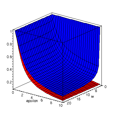
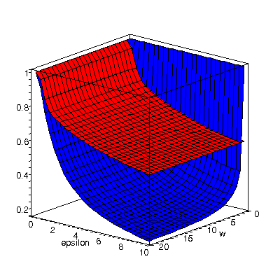
Figure 1: Behavior of $\varrho$ in $(\mathbb{R}^{d+1},\ell_{1})$. Left: plots of $\varrho$ (blue) and $\frac{1}{1+\varepsilon^{\prime}}=\frac{1}{1+\varepsilon^{2}/(1+\varepsilon)}$ (red) versus $\varepsilon$ and $w$. Right: plots of $\varrho$ (blue) and $\frac{1}{1+\min\{\varepsilon^{2},\;\sqrt{\varepsilon}\}/4}$ (red) versus $\varepsilon$ and $w$.

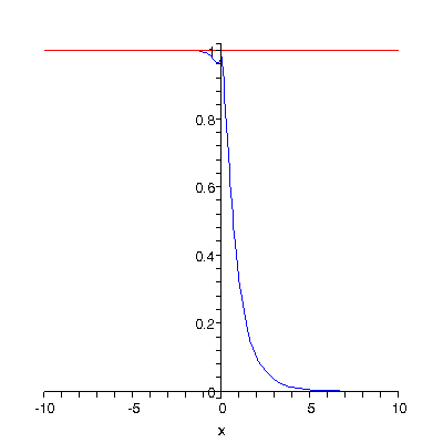
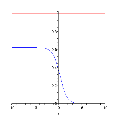
Figure 2: Behaviors of $\varrho$ and $\alpha$ in $(\mathbb{R}^{d+1},\ell_{1})$ after letting $w=\max\{1,\varepsilon\}$. From left to right, in blue: plots of $\varrho(1+\min\{\varepsilon^{2},\;\sqrt{\varepsilon}\}/4)$ and $\frac{\alpha}{\varepsilon\varrho}$. Both plots are versus $\varepsilon$ on a logarithmic scale ($x=\log_{10}\varepsilon$). The red lines have equation $y=1$.

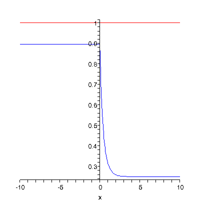
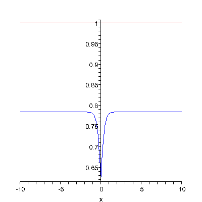
Figure 3: Behaviors of $\frac{1}{\Phi(1)}$ and $\frac{1}{\ln\nicefrac{{1}}{{\Phi(1+\varepsilon^{\prime})}}}$ in $(\mathbb{R}^{d+1},\ell_{1})$ after letting $w=\max\{1,\varepsilon\}$. From left to right, in blue: plots of $\frac{1}{4\Phi(1)}$ and $\frac{1}{\ln\nicefrac{{1}}{{\Phi(1+\varepsilon^{\prime})}}}$. Both plots are versus $\varepsilon$ on a logarithmic scale ($x=\log_{10}\varepsilon$). The red lines have equation $y=1$.

Case $s=1$.

The definition of $\varepsilon^{\prime}$ gives $\varepsilon^{\prime}=\frac{\varepsilon^{2}}{1+\varepsilon}$ in this case. The formula for $\varrho$ is then the same as in $\mathbb{R}^{d}$, with $\varepsilon$ replaced by $\frac{\varepsilon^{2}}{1+\varepsilon}$. As reported in [11] and illustrated in Figure 1 (left), $\varrho$ remains above $\frac{1}{1+\varepsilon^{2}/(1+\varepsilon)}$, even though it seems to converge to this quantity as $w$ tends to infinity. Letting $w=\max\{1,\varepsilon\}$, we found experimentally that $\varrho$ is dominated by $\frac{1}{1+\varepsilon^{2}/4}$ when $\varepsilon\leq 1$ and by $\frac{1}{1+\sqrt{\varepsilon}/4}$ when $\varepsilon\geq 1$, as shown in Figures 1 (right) and 2 (left). In the meantime, $\alpha$ is less than $\varepsilon\varrho$, as can be seen from Figure 2 (right), while $\frac{1}{\Phi(1)}$ and $\frac{1}{\ln\nicefrac{{1}}{{\Phi(1+\varepsilon^{\prime})}}}$ are less than $4$ and $1$ respectively, as shown in Figure 3. All in all, Theorem 3.7 can be re-written as follows:

Theorem 3.7 (case $s=1$).

Given a finite set $P$ with $n$ points in $(\mathbb{R}^{d},\ell_{1})$, and two parameters $r,\varepsilon>0$, the $\mathcal{A}^{\prime}(P,r,\varepsilon)$ data structure answers exhaustive $r$-$\mathcal{PLEB}$ queries correctly with high probability in expected $\tilde{O}(n^{\varrho}+n^{\alpha}|\mathcal{B}_{P}(q,r(1+\varepsilon))|)$ time using $\tilde{O}(n^{1+\varrho})$ space, where $\varrho\leq\frac{1}{1+\min\{\varepsilon^{2},\;\sqrt{\varepsilon}\}/4}<1$ and $\alpha\leq\varepsilon\varrho<\varepsilon$.

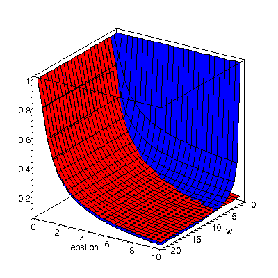
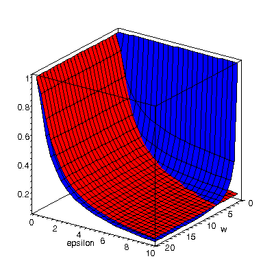
Figure 4: Behavior of $\varrho$ in $(\mathbb{R}^{d+1},\ell_{2})$. Left: plots of $\varrho$ (blue) and $\frac{1}{1+\varepsilon^{\prime}}=\frac{1+\varepsilon}{\sqrt{(1+\varepsilon)^{4}-1}}$ (red) versus $\varepsilon$ and $w$. Right: plots of $\varrho$ (blue) and $\frac{1}{1+\varepsilon^{2}/(1+\varepsilon)}$ (red) versus $\varepsilon$ and $w$.

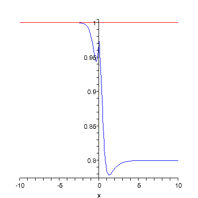
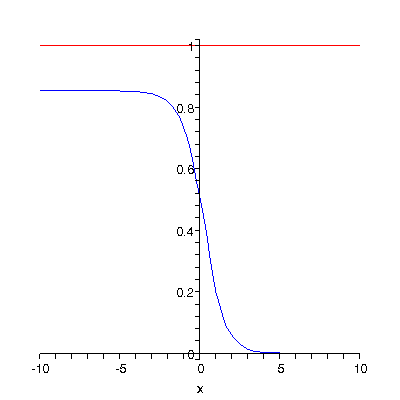
Figure 5: Behaviors of $\varrho$ and $\alpha$ in $(\mathbb{R}^{d+1},\ell_{2})$ after letting $w=\max\{1,\varepsilon\}$. From left to right, in blue: plots of $\varrho(1+\varepsilon^{2}/(1+\varepsilon))$ and $\frac{\alpha}{\varepsilon\varrho}$. Both plots are versus $\varepsilon$ on a logarithmic scale ($x=\log_{10}\varepsilon$). The red lines have equation $y=1$.

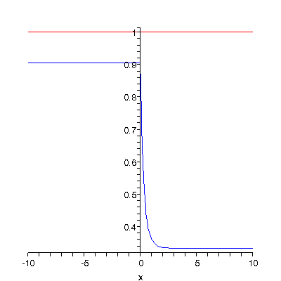
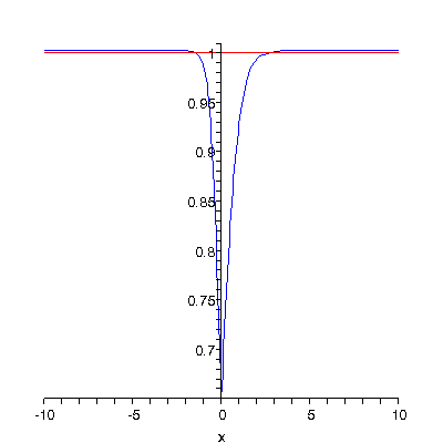
Figure 6: Behaviors of $\frac{1}{\Phi(1)}$ and $\frac{1}{\ln\nicefrac{{1}}{{\Phi(1+\varepsilon^{\prime})}}}$ in $(\mathbb{R}^{d+1},\ell_{2})$ after letting $w=\max\{1,\varepsilon\}$. From left to right, in blue: plots of $\frac{1}{3\Phi(1)}$ and $\frac{1}{\ln\nicefrac{{1}}{{\Phi(1+\varepsilon^{\prime})}}}$. Both plots are versus $\varepsilon$ on a logarithmic scale ($x=\log_{10}\varepsilon$). The red lines have equation $y=1$.

Case $s=2$.

The definition of $\varepsilon^{\prime}$ gives $\varepsilon^{\prime}=\frac{\sqrt{(1+\varepsilon)^{4}-1}}{1+\varepsilon}-1$ in this case. The formula for $\varrho$ is then the same as in $\mathbb{R}^{d}$, with $\varepsilon$ replaced by $\frac{\sqrt{(1+\varepsilon)^{4}-1}}{1+\varepsilon}-1$. As pointed out in [11] and illustrated in Figure 4 (left), $\varrho$ goes below $\frac{1+\varepsilon}{\sqrt{(1+\varepsilon)^{4}-1}}$ at reasonably small values of parameter $w$. Since this bound is not quite evocative, we used a slightly different bound, namely $\frac{1}{1+\varepsilon^{2}/(1+\varepsilon)}$, and we found experimentally that $\varrho\leq\frac{1}{1+\varepsilon^{2}/(1+\varepsilon)}$ whenever $w=\max\{1,\varepsilon\}$, as shown in Figures 4 (right) and 5 (left). In the meantime, $\alpha$ is less than $\varepsilon\varrho$, as can be seen from Figure 5 (right), while the terms $\frac{1}{\Phi(1)}$ and $\frac{1}{\ln\nicefrac{{1}}{{\Phi(1+\varepsilon^{\prime})}}}$ are bounded by small constants, as shown in Figure 6. All in all, Theorem 3.7 can be re-written as follows:

Theorem 3.7 (case $s=2$).

Given a finite set $P$ with $n$ points in $(\mathbb{R}^{d},\ell_{2})$, and two parameters $r,\varepsilon>0$, the $\mathcal{A}^{\prime}(P,r,\varepsilon)$ data structure answers exhaustive $r$-$\mathcal{PLEB}$ queries correctly with high probability in expected $\tilde{O}(n^{\varrho}+n^{\alpha}|\mathcal{B}_{P}(q,r(1+\varepsilon))|)$ time using $\tilde{O}(n^{1+\varrho})$ space, where $\varrho\leq\frac{1}{1+\varepsilon^{2}/(1+\varepsilon)}<1$ and $\alpha\leq\varepsilon\varrho<\varepsilon$.

4 Interlude: from exhaustive $r$-$\mathcal{PLEB}$ to exact $\mathcal{NN}$

Before dealing with $\mathcal{RNN}$ queries (the main topic of the paper), let us show a simple but pedagogical application of exhaustive $r$-$\mathcal{PLEB}$ queries to exact $\mathcal{NN}$ search. Given a set $P$ with $n$ points and a user-defined parameter $\varepsilon>0$, we will show that $\mathcal{NN}$ queries can be solved exactly with high probability on any query point $q$ in expected $\tilde{O}(n^{\varrho}+n^{\alpha}|O(\varepsilon)\mbox{-}\mathcal{NN}_{P}(q)|)$ time using $\tilde{O}(n^{1+\varrho})$ space, for some quantities $\varrho=\frac{1}{1+\Theta(\varepsilon^{2})}<1$ and $\alpha\leq\varepsilon\varrho<\varepsilon$ (Theorem 4.3). The running time bound is composed of two terms: the first one is sublinear in $n$ and corresponds to a standard approximate $\varepsilon$-$\mathcal{NN}$ query using locality-sensitive hashing; the second one depends on the size of the approximate nearest neighbors set $O(\varepsilon)\mbox{-}\mathcal{NN}_{P}(q)$ and indicates that the solution to the exact query is sought for among this set. Whether the bound will be sublinear in $n$ or not in the end depends on the size of the set compared to the quantity $n^{1-\alpha}$. This follows the intuition that finding the exact nearest neighbor of $q$ is easy when $q$ does not have too many approximate nearest neighbors, and in this respect the quantity $|O(\varepsilon)\mbox{-}\mathcal{NN}_{P}(q)|$ plays the role of a condition number measuring the inherent difficulty of a given instance of the exact $\mathcal{NN}$ problem. The interesting point to raise here is that the limit on this number for our algorithm to be sublinear is at least of the order of $n^{1-\varepsilon}$ since we have $\alpha<\varepsilon$.

Let us point out that the above bounds are for the ambient space $\mathbb{R}^{d}$ equipped with the $\ell_{1}$- or $\ell_{2}$-norm. Our analysis will be carried out in the more general setting of an $\ell_{s}$-norm, with $s\in(0,2]$, where we will derive more general complexity bounds. The choice of $(\mathbb{R}^{d},\ell_{s})$ is mainly for ease of exposition, since the algorithm can actually be applied in arbitrary metric spaces that admit locality-sensitive families of hash functions, where its analysis extends in a straightforward manner (see Remark 4.4 at the end of the section).

The algorithm.

Let $P$ be a finite set of $n$ points in $(\mathbb{R}^{d},\ell_{s})$, $s\in(0,2]$, and let $\varepsilon>0$ be a parameter. The preprocessing phase consists of the following steps:

• Build the tree structure $\mathcal{T}(P,\varepsilon)$ of Section 2.2 and its associated $(r,\varepsilon)$-$\mathcal{PLEB}$ data structures.

• For every $(r,\varepsilon)$-$\mathcal{PLEB}$ data structure built on some subset of $P$ at step i, build an $\mathcal{A}^{\prime}(P,r,\varepsilon)$ data structure using the procedure of Section 3.2.

Then, given a query point $q$, we proceed as follows:

• Answer an $\varepsilon$-$\mathcal{NN}$ query using the tree structure $\mathcal{T}(P,\varepsilon)$, and let $r\geq 0$ be the output value.

• Answer an exhaustive $r$-$\mathcal{PLEB}$ query using the $\mathcal{A}^{\prime}(P,r,\varepsilon)$ data structure, and let $S$ be the output set.

• Iterate over the points of $S$ and return the one that is closest to $q$. If $S$ is empty, then return any arbitrary point of $P$.

Note that the execution of step 2 is made possible by the fact that the algorithm solving the $\varepsilon$-$\mathcal{NN}$ query at step 1 returns a radius $r$ that is stored in one of the $\mathcal{A}^{\prime}(P,r,\varepsilon)$ data structures built during the preprocessing phase. For any other value $r$ we would not be able to perform step 2 because we would not have the corresponding $\mathcal{A}^{\prime}(P,r,\varepsilon)$ data structure at hand.

Analysis.

We begin by showing the correctness of the query procedure:

Lemma 4.1.

The query procedure returns a point of $\mathcal{NN}_{P}(q)$ with high probability.

Proof.

Corollary 2.4 guarantees that the radius $r$ computed at step 1 satisfies $\mathrm{d}(q,P)\leq r\leq\mathrm{d}(q,P)(1+\varepsilon)$ with high probability. Under this condition, we have $\mathcal{NN}_{P}(q)\subseteq\mathcal{B}_{P}(q,r)$, and so Theorem 3.7 guarantees that the set $S$ computed at step 2 contains $\mathcal{NN}_{P}(q)$ with high probability. It follows that the point returned at step 3 belongs to $\mathcal{NN}_{P}(q)$ with high probability. ∎

We will now analyze the expected running time of the query. Let $D$ be the $s$-stable distribution used by the algorithm, and let $p_{0}=\Phi(\frac{1}{1+\varepsilon})$, $p_{1}=\Phi(1)$, $p_{2}=\Phi(1+\varepsilon)$ and $p^{\prime}_{2}=\Phi(((1+\varepsilon)^{s}+(1+\varepsilon)^{-s}-1)^{1/s})$ be derived from $D$ according to Eq. (1). By Corollary 2.4, the running time of step 1 is $\tilde{O}(\frac{n^{\varrho}}{p_{1}\ln\nicefrac{{1}}{{p_{2}}}})$, where $\varrho=\frac{\ln p_{1}}{\ln p_{2}}$. The running time of step 3 is $O(|S|)$, so it is dominated by the running time of step 2.

Lemma 4.2.

The expected running time of step 2 is $\tilde{O}(\frac{n^{\varrho^{\prime}}}{p_{1}}(\frac{1}{\ln\nicefrac{{1}}{{p^{\prime}_{2}}}}+1)+\frac{n^{\alpha}}{p_{1}}|\varepsilon(2+\varepsilon)\mbox{-}\mathcal{NN}_{P}(q)|)$, where $\varrho^{\prime}=\frac{\ln p_{1}}{\ln p^{\prime}_{2}}$ and $\alpha=\varrho^{\prime}(1-\frac{\ln p_{0}}{\ln p_{1}})$.

Proof.

Let $r$ be the radius computed at step 1. By Theorem 3.7, the expected running time of step 2 is $\tilde{O}(\frac{n^{\varrho^{\prime}}}{p_{1}}(\frac{1}{\ln\nicefrac{{1}}{{p^{\prime}_{2}}}}+1)+\frac{n^{\alpha}}{p_{1}}|\mathcal{B}_{P}(q,r(1+\varepsilon))|)$. If $r\leq\mathrm{d}(q,P)(1+\varepsilon)$, then we have $\mathcal{B}_{P}(q,r(1+\varepsilon))\subseteq\varepsilon(2+\varepsilon)\mbox{-}\mathcal{NN}_{P}(q)$ and so the expected running time becomes $\tilde{O}(\frac{n^{\varrho^{\prime}}}{p_{1}}(\frac{1}{\ln\nicefrac{{1}}{{p^{\prime}_{2}}}}+1)+\frac{n^{\alpha}}{p_{1}}|\varepsilon(2+\varepsilon)\mbox{-}\mathcal{NN}_{P}(q)|)$. By contrast, if $r>\mathrm{d}(q,P)(1+\varepsilon)$, then we have no bound on the size of $\mathcal{B}_{P}(q,r(1+\varepsilon))$ other than $n$, so the expected running time of step 2 becomes $\tilde{O}(\frac{n^{\varrho^{\prime}}}{p_{1}}(\frac{1}{\ln\nicefrac{{1}}{{p^{\prime}_{2}}}}+1)+\frac{n^{\alpha+1}}{p_{1}})$. Now, recall from Section 2 that the event that $r>\mathrm{d}(q,P)(1+\varepsilon)$ only occurs with very low probability, more precisely with probability at most $\frac{1}{n}$. Therefore, in total the expected running time of step 2 is bounded by $\tilde{O}(\frac{n^{\varrho^{\prime}}}{p_{1}}(\frac{1}{\ln\nicefrac{{1}}{{p^{\prime}_{2}}}}+1)+\frac{n^{\alpha}}{p_{1}}|\varepsilon(2+\varepsilon)\mbox{-}\mathcal{NN}_{P}(q)|+\frac{1}{n}\frac{n^{\alpha+1}}{p_{1}})$, which is $\tilde{O}(\frac{n^{\varrho^{\prime}}}{p_{1}}(\frac{1}{\ln\nicefrac{{1}}{{p_{2}}}}+1)+\frac{n^{\alpha}}{p_{1}}|\varepsilon(2+\varepsilon)\mbox{-}\mathcal{NN}_{P}(q)|)$ since the set $\varepsilon(2+\varepsilon)\mbox{-}\mathcal{NN}_{P}(q)$ contains at least one point, namely the nearest neighbor of $q$. ∎

Let us now focus on the size of the data structure. By Corollary 2.4, the total size of the tree $\mathcal{T}(P,\varepsilon)$ and associated $(r,\varepsilon)$-$\mathcal{PLEB}$ data structures is $\tilde{O}(\frac{1}{\varepsilon}\frac{n^{1+\varrho}}{p_{1}})$. In addition, since $\mathcal{T}(P,\varepsilon)$ has $\tilde{O}(n)$ nodes in total, each one storing $\tilde{O}(\frac{1}{\varepsilon})$ data structures for $(r,\varepsilon)$-$\mathcal{PLEB}$, the total number of $\mathcal{A}^{\prime}(P,r,\varepsilon)$ data structures built at step ii of the preprocessing phase is $\tilde{O}(\frac{n}{\varepsilon})$. Therefore, by Theorem 3.7, the total memory usage of the $\mathcal{A}^{\prime}(P,r,\varepsilon)$ data structures is $\tilde{O}(\frac{1}{\varepsilon}\frac{n^{2+\varrho^{\prime}}}{p_{1}})$.

Observing now that we have $p^{\prime}_{2}\geq p_{2}$ and $\varrho^{\prime}\geq\varrho$ since $((1+\varepsilon)^{s}+(1+\varepsilon)^{-s}-1)^{1/s}\leq 1+\varepsilon$, we conclude that our procedure has the following space and time complexities (where $p^{\prime}_{2}$ and $\varrho^{\prime}$ have been renamed respectively $p_{2}$ and $\varrho$ for convenience):

Theorem 4.3.

Given a finite set $P$ with $n$ points in $(\mathbb{R}^{d},\ell_{s})$, $s\in(0,2]$, and a user-defined parameter $\varepsilon>0$, our procedure answers exact $\mathcal{NN}$ queries with high probability in expected $\tilde{O}(\frac{n^{\varrho}}{p_{1}}(\frac{1}{\ln\nicefrac{{1}}{{p_{2}}}}+1)+\frac{n^{\alpha}}{p_{1}}|\varepsilon(2+\varepsilon)\mbox{-}\mathcal{NN}_{P}(q)|)$ time using $\tilde{O}(\frac{1}{\varepsilon}\frac{n^{2+\varrho}}{p_{1}})$ space, where $\varrho=\frac{\ln p_{1}}{\ln p_{2}}$ and $\alpha=\varrho(1-\frac{\ln p_{0}}{\ln p_{1}})$, the quantities $p_{0}=\Phi(\frac{1}{1+\varepsilon})$, $p_{1}=\Phi(1)$ and $p_{2}=\Phi(((1+\varepsilon)^{s}+(1+\varepsilon)^{-s}-1)^{1/s})$ being derived from some $s$-stable distribution $D$ according to Eq. (1).

Replacing Theorem 3.7 by its specialized versions for $s=1$ and $s=2$ in the analysis immediately gives the following complexity bounds:

Theorem 4.3 (case $s=1$).

Given a finite set $P$ with $n$ points in $(\mathbb{R}^{d},\ell_{1})$, and a user-defined parameter $\varepsilon>0$, our procedure answers exact $\mathcal{NN}$ queries with high probability in expected $\tilde{O}(n^{\varrho}+n^{\alpha}|\varepsilon(2+\varepsilon)\mbox{-}\mathcal{NN}_{P}(q)|)$ time using $\tilde{O}(\frac{1}{\varepsilon}n^{2+\varrho})$ space, where $\varrho\leq\frac{1}{1+\min\{\varepsilon^{2},\;\sqrt{\varepsilon}\}/4}<1$ and $\alpha\leq\varepsilon\varrho<\varepsilon$.

Theorem 4.3 (case $s=2$).

Given a finite set $P$ with $n$ points in $(\mathbb{R}^{d},\ell_{2})$, and a user-defined parameter $\varepsilon>0$, our procedure answers exact $\mathcal{NN}$ queries with high probability in expected $\tilde{O}(n^{\varrho}+n^{\alpha}|\varepsilon(2+\varepsilon)\mbox{-}\mathcal{NN}_{P}(q)|)$ time using $\tilde{O}(\frac{1}{\varepsilon}n^{2+\varrho})$ space, where $\varrho\leq\frac{1}{1+\varepsilon^{2}/(1+\varepsilon)}<1$ and $\alpha\leq\varepsilon\varrho<\varepsilon$.

Note that in practice a trade-off must be made by the user when choosing parameter $\varepsilon$. Indeed, the smaller $\varepsilon$, the smaller the set $\varepsilon(2+\varepsilon)\mbox{-}\mathcal{NN}_{P}(q)$ and the smaller $\alpha$ compared to $\varrho$, but on the other hand the higher $\varrho$ itself.

Remark 4.4.

In our analysis we traded optimality for simplicity since we applied the results from Section 3.2 verbatim. In fact, a closer look at the problem reveals that the points of $P$ lie at least $\mathrm{d}(q,P)\geq\frac{r}{1+\varepsilon}$ away from the query point $q$ with high probability at step 2 of the query phase. This means that no lifting of the data into $\mathbb{R}^{d+1}$ is actually needed. We then have $p^{\prime}_{2}=p_{2}$, $\varrho^{\prime}=\varrho$, and a careful analysis shows that relevant choices of parameter $w$ reduce $\varrho$ down to (or at least close to) $\frac{1}{1+\varepsilon}$. In addition and more importantly, not having to re-embed the data means that the algorithm can be applied in arbitrary metric spaces $(X,\mathrm{d})$ that admit locality-sensitive families of hash functions, where the analysis extends in a straightforward manner.

5 From exhaustive $r$-$\mathcal{PLEB}$ to exact $\mathcal{RNN}$

In this section we focus on our main problem ($\mathcal{RNN}$) and show how it can be reduced to a single instance of $\varepsilon$-$\mathcal{NN}$ search plus a controlled number of instances of exhaustive $r$-$\mathcal{PLEB}$. Although the reduction is applicable in any metric space, we will restrict our study to the case of $\mathbb{R}^{d}$ equipped with an $\ell_{s}$-norm, $s\in(0,2]$, where the non-isometric embedding trick of Section 3.2 can be used to speed-up the process. The details of the reduction are given in Section 5.2, its output proven correct in Section 5.3, and its complexity analyzed in Section 5.4. The reduction and analysis are then extended to the bichromatic setting in Section 5.5. For now we begin with an overview of the reduction and of its key ingredients in Section 5.1.

5.1 Overview of the reduction

Let $P$ be a finite set with $n$ points in $(\mathbb{R}^{d},\ell_{s})$, $s\in(0,2]$. Suppose the distance of every point $p\in P$ to its nearest neighbor in $P\setminus\{p\}$ has been pre-computed. Then, given a query point $q$, computing a solution to the $\mathcal{RNN}$ query amounts to checking, for every point $p\in P$, whether $\mathrm{d}(q,p)\leq\mathrm{d}(p,P)$ or $\mathrm{d}(q,p)>\mathrm{d}(p,P)$: in the first case, $p$ must be included in the solution, whereas in the second case it must not. This check for point $p$ can be done by computing the solution $S$ of the exaustive $r$-$\mathcal{PLEB}$ query on input $(P,q)$, with $r=\mathrm{d}(p,P)$, and by including $p$ in the answer if and only if it belongs to $S$. Indeed,

$$p\in\mathcal{RNN}_{P}(q)\Leftrightarrow\mathrm{d}(p,q)\leq\mathrm{d}(p,P)=r\Leftrightarrow p\in\mathcal{B}_{P}(q,r)\Leftrightarrow p\in S.$$

Thus, computing the set $\mathcal{RNN}_{P}(q)$ boils down to locating $q$ among the set of balls $\{\mathcal{B}(p,\mathrm{d}(p,P))\mid p\in P\}$. This observation was exploited in previous work [23] and serves as the starting point of our approach. The main problem is that the ball radius $r$ changes with each data point $p\in P$ considered, so the total number of exhaustive $r$-$\mathcal{PLEB}$ queries to be solved can be up to linear in $n$. To reduce this number, we allow some degree of fuzziness and use a bucketing strategy. Given a user-defined parameter $\varepsilon>0$, at pre-processing time we compute and store $\mathrm{d}(p,P)$ for every point $p\in P$ and then we hash the data points into buckets according to their nearest neighbor distances, so that bucket $P_{i}$ contains the points $p\in P$ such that $(1+\varepsilon)^{i-1}\leq\mathrm{d}(p,P)<(1+\varepsilon)^{i}$. At query time, we solve an exhaustive $r$-$\mathcal{PLEB}$ query with $r=(1+\varepsilon)^{i}$ on each bucket $P_{i}$ separately, then we consider the union $S$ of the solutions and prune out those points $p\in S$ such that $\mathrm{d}(p,q)>\mathrm{d}(p,P)$. Since the points $p\in P_{i}$ satisfy $(1+\varepsilon)^{i-1}\leq\mathrm{d}(p,P)<(1+\varepsilon)^{i}$, it is easily seen that $\mathcal{RNN}_{P}(q)\subseteq S\subseteq\varepsilon\mbox{-}\mathcal{RNN}_{P}(q)$ and that our output is an admissible solution to the $\mathcal{RNN}$ query.

A remaining issue is that we do not impose any constraints on parameter $i$, so at query time we need to inspect every single non-empty bucket $P_{i}$. As a result, in pathological cases such as when all non-empty buckets are singletons, we will end up considering a linear number of buckets, even though the set $\varepsilon\mbox{-}\mathcal{RNN}_{P}(q)$ itself might be small or even empty. To avoid this pitfall, we limit the range of values of $i$ to be considered thanks to the following observations, where $y$ is an arbitrary point of $\varepsilon\mbox{-}\mathcal{NN}_{P}(q)$:

Observation 1.

Every point $p\in\mathcal{RNN}_{P}(q)$ satisfies $\mathrm{d}(p,P)\geq\frac{\mathrm{d}(q,y)}{1+\varepsilon}$.

Proof.

Since $p\in\mathcal{RNN}_{P}(q)$, we have $p\neq q$ and $\mathrm{d}(p,q)\leq\mathrm{d}(p,P)$. Moreover, since $p\neq q$ and $y\in\varepsilon\mbox{-}\mathcal{NN}_{P}(q)$, we have $\mathrm{d}(q,y)\leq(1+\varepsilon)\mathrm{d}(q,P)\leq(1+\varepsilon)\mathrm{d}(q,p)$. It follows that $\mathrm{d}(q,y)\leq(1+\varepsilon)\mathrm{d}(p,P)$. ∎

Observation 2.

Every point $p\in\mathcal{RNN}_{P}(q)$ such that $\mathrm{d}(p,P)\geq\frac{\mathrm{d}(q,y)}{\varepsilon}$ belongs to $\varepsilon\mbox{-}\mathcal{RNN}_{P}(y)\cup\{y\}$.

Proof.

Since $p\in\mathcal{RNN}_{P}(q)$, we have $\mathrm{d}(p,q)\leq\mathrm{d}(p,P)$. In addition, we have $\mathrm{d}(q,y)\leq\varepsilon\,\mathrm{d}(p,P)$ by hypothesis. Hence, $\mathrm{d}(p,y)\leq\mathrm{d}(p,q)+\mathrm{d}(q,y)\leq(1+\varepsilon)\mathrm{d}(p,P)$, which means that either $p=y$ or $p\in\varepsilon\mbox{-}\mathcal{RNN}_{P}(y)$. ∎

Assuming that we have precomputed a data structure that enables us to find some $y\in\varepsilon\mbox{-}\mathcal{NN}_{P}(q)$, Observation 1 ensures that we can safely ignore the buckets $P_{i}$ with $i\leq\log_{1+\varepsilon}\frac{\mathrm{d}(q,y)}{1+\varepsilon}$. Furthermore, assuming that the set $\varepsilon\mbox{-}\mathcal{RNN}_{P}(y)$ has been precomputed, Observation 2 ensures that the reverse nearest neighbors of $q$ that belong to the buckets $P_{i}$ with $i\geq 1+\log_{1+\varepsilon}\frac{\mathrm{d}(q,y)}{\varepsilon}$ can simply be looked for among the points of $\varepsilon\mbox{-}\mathcal{RNN}_{P}(y)\cup\{y\}$. Thus, the total number of buckets to be inspected is reduced to $O(\frac{1}{\varepsilon}\log\frac{1}{\varepsilon})=\tilde{O}(\frac{1}{\varepsilon})$.

5.2 Details of the reduction

Given a finite set $P$ with $n$ points in $(\mathbb{R}^{d},\ell_{s})$, $s\in(0,2]$, and a parameter $\varepsilon>0$, our pre-computation phase builds a data structure $\mathcal{RNNDS}(P,\varepsilon)$ that stores the following pieces of information:

• A collection of buckets $\{P_{i}\}_{i\in\mathbb{Z}}$ that partition $P$. Each bucket $P_{i}$ contains those points $p\in P$ such that $(1+\varepsilon)^{i-1}\leq\mathrm{d}(p,P)<(1+\varepsilon)^{i}$. To fill in the buckets, we iterate over the points $p\in P$, we compute the distance $\mathrm{d}(p,P)$ exactly and store it, and then we assign $p$ to its corresponding bucket. Once this is done, the empty buckets are discarded and the non-empty buckets are stored in a hash table to ensure constant look-up time. On each non-empty bucket $P_{i}$ we build an $\mathcal{A}^{\prime}(P_{i},(1+\varepsilon)^{i},\varepsilon)$ data structure using the procedure of Section 3.2. Note that when applying Algorithm 1 we increase the number of iterations of the main loop from $\lceil c\ln|P_{i}|\rceil$ to $\lceil c\ln n\rceil$, where $c=\frac{3}{\ln\frac{5}{2}}$.

• For each point $y\in P$, an array $P_{y}$ containing the points $p\in\varepsilon\mbox{-}\mathcal{RNN}_{P}(y)\cup\{y\}$, sorted by increasing distances $\mathrm{d}(p,P)$. Building the array takes $\tilde{O}(n)$ time once $\mathrm{d}(p,P)$ has been computed for all $p\in P$.

• The tree $\mathcal{T}(P,\varepsilon)$ of Section 2.2 and its associated $(r,\varepsilon)$-$\mathcal{PLEB}$ data structures.

Given a point $q\in\mathbb{R}^{d}$, we answer the $\mathcal{RNN}$ query using the $\mathcal{RNNDS}(P,\varepsilon)$ data structure as follows:

• We use the tree $\mathcal{T}(P,\varepsilon)$ and its associated $(r,\varepsilon)$-$\mathcal{PLEB}$ data structures to answer an $\varepsilon$-$\mathcal{NN}$ query, and we let $y$ be the output point.

• We use the $\mathcal{A}^{\prime}(P_{i},(1+\varepsilon)^{i},\varepsilon)$ data structure to answer an exhaustive $(1+\varepsilon)^{i}$-$\mathcal{PLEB}$ query on each bucket $P_{i}$ separately, for $i$ lying in the range prescribed by Observations 1 and 2, and then we merge the output sets into a single set $S$. Note that when applying Algorithm 2 on $P_{i}$ we increase the number of iterations of the main loop from $\lceil c\ln|P_{i}|\rceil$ to $\lceil c\ln n\rceil$, where $c=\frac{3}{\ln\frac{5}{2}}$, which raises the probability of success of the query from $1-\frac{1}{|P_{i}|^{2}}$ (which can be as low as $0$ when $P_{i}$ is a singleton) to $1-\frac{1}{n^{2}}$.

• We add to $S$ the points $p\in\varepsilon\mbox{-}\mathcal{RNN}_{P}(y)\cup\{y\}$ s.t. $\mathrm{d}(p,P)\geq\frac{\mathrm{d}(q,y)}{\varepsilon}$. These are found by looking up the value $\frac{\mathrm{d}(q,y)}{\varepsilon}$ in the sorted array $P_{y}$ by binary search, and then by iterating until the end of the array.

• We iterate over the points $p\in S$ and remove the ones that do not satisfy $\mathrm{d}(p,q)\leq\mathrm{d}(p,P)$.

Upon termination, we return the set $S$. The pseudo-codes of the preprocessing and query procedures are given in Algorithms 3 and 4.

Input : point cloud $P\subset\mathbb{R}^{d}$, parameter $\varepsilon>0$

Output : $\mathcal{RNNDS}(P,\varepsilon)$ data structure

1

2Initialize $P_{i}:=\emptyset$ for $i\in\mathbb{Z}$;

3 foreach $p\in P$ do

4       Compute $\mathrm{d}(p,P)$ exactly and store it;

5       Find $i$ s.t. $(1+\varepsilon)^{i-1}\leq\mathrm{d}(p,P)<(1+\varepsilon)^{i}$ and update $P_{i}:=P_{i}\cup\{p\}$;

6      

7 end foreach

8foreach $P_{i}\neq\emptyset$ do

9       Build an $\mathcal{A}^{\prime}(P_{i},(1+\varepsilon)^{i},\varepsilon)$ data structure;

10      

11 end foreach

12foreach $y\in P$ do

13       Build the set $\varepsilon\mbox{-}\mathcal{RNN}_{P}(y)\cup\{y\}$ and store it in an array $P_{y}$ ;

14       Sort the points $p\in P_{y}$ by increasing distances $\mathrm{d}(p,P)$ ;

15      

16 end foreach

17Build the tree $\mathcal{T}(P,\varepsilon)$ of Section 2.2 and its associated $(r,\varepsilon)$-$\mathcal{PLEB}$ data structures ;

Algorithm 3 Pre-processing phase for $\mathcal{RNN}$.

Input : $\mathcal{RNNDS}(P,\varepsilon)$ data structure, query point $q\in\mathbb{R}^{d}$

1

2Answer an $\varepsilon$-$\mathcal{NN}$ query on input $(P,q)$, and let $y$ be the output ;

3 for $i=\left\lfloor\log_{1+\varepsilon}\frac{\mathrm{d}(q,y)}{1+\varepsilon}\right\rfloor+1\ \mathrm{to}\ \left\lceil\log_{1+\varepsilon}\frac{\mathrm{d}(q,y)}{\varepsilon}\right\rceil$ do

4       if $P_{i}\neq\emptyset$ then

5             Answer an exhaustive $(1+\varepsilon)^{i}$-$\mathcal{PLEB}$ query on input $(P_{i},q)$, and let $S_{i}$ be the output ;

6            

7       end if

8      

9 end for

10

11Let $S:=\bigcup_{i}S_{i}$ ;

12

13Look up the value $\frac{\mathrm{d}(q,y)}{\varepsilon}$ in the sorted array $P_{y}$ by binary search ;

14

15Iterate from the value $\frac{\mathrm{d}(q,y)}{\varepsilon}$ to the end of the array $P_{y}$ and insert all the visited points into $S$ ;

16

17foreach $p\in S$  do

18       if $\mathrm{d}(p,q)>\mathrm{d}(p,P)$ then

19             Remove $p$ from $S$;

20            

21       end if

22      

23 end foreach

24

25Return $S$ ;

Algorithm 4 Online query phase for $\mathcal{RNN}$.

5.3 Correctness of the output

Corollary 2.4 guarantees that step 1 of the query procedure retrieves a point $y\in\varepsilon\mbox{-}\mathcal{NN}_{P}(q)$ with high probability. Let us show that, given that $y\in\varepsilon\mbox{-}\mathcal{NN}_{P}(q)$, the final set $S$ output by the query procedure satisfies $S=\mathcal{RNN}_{P}(q)$ with high probability. For clarity, we let $S^{\prime}$ be the set of points inserted in $S$ at step 2 of the procedure, and $S^{\prime\prime}$ be the set of points inserted at step 3. The output of the algorithm is then $(S^{\prime}\cup S^{\prime\prime})\cap\mathcal{RNN}_{P}(q)$. Let $P^{\prime}=\bigcup_{i}P_{i}$ for $i=\lfloor\log_{1+\varepsilon}\frac{\mathrm{d}(q,y)}{1+\varepsilon}\rfloor+1$ to $\lceil\log_{1+\varepsilon}\frac{\mathrm{d}(q,y)}{\varepsilon}\rceil$.

Lemma 5.1.

$\mathcal{RNN}_{P}(q)\cap P^{\prime}\subseteq S^{\prime}$ with high probability.

Proof.

Step 2 of the query procedure builds $S^{\prime}$ by taking the union of the sets $S_{i}$ generated by answering exhaustive $(1+\varepsilon)^{i}$-$\mathcal{PLEB}$ queries on the non-empty buckets $P_{i}$ with query point $q$. For each such $P_{i}$, we have $\mathcal{RNN}_{P}(q)\cap P_{i}\subseteq\mathcal{B}_{P_{i}}(q,(1+\varepsilon)^{i})$ since by definition every point $p\in\mathcal{RNN}_{P}(q)\cap P_{i}$ satisfies $\mathrm{d}(p,q)\leq\mathrm{d}(p,P)\leq(1+\varepsilon)^{i}$. Now, by Theorem 3.2, we have $S_{i}=\mathcal{B}_{P_{i}}(q,(1+\varepsilon)^{i})$ with probability at least $1-\frac{1}{n^{2}}$. Thus, $\mathcal{RNN}_{P}(q)\cap P_{i}\subseteq S_{i}$ with probability at least $1-\frac{1}{n^{2}}$. Since the total number of non-empty buckets is at most $n$, the union bound tells us that $\mathcal{RNN}_{P}(q)\cap P^{\prime}\subseteq S^{\prime}$ with probability at least $1-\frac{1}{n}$. ∎

Lemma 5.2.

Given that $y\in\varepsilon\mbox{-}\mathcal{NN}_{P}(q)$, we have $\mathcal{RNN}_{P}(q)\setminus P^{\prime}\subseteq S^{\prime\prime}$ with high probability.

Proof.

The result follows from Observations 1 and 2. Indeed, every point $p\in P_{i}$ with $i<\lfloor\log_{1+\varepsilon}\frac{\mathrm{d}(q,y)}{1+\varepsilon}\rfloor+1$ satisfies $\mathrm{d}(p,P)<(1+\varepsilon)^{i}\leq\frac{\mathrm{d}(q,y)}{1+\varepsilon}$ and therefore cannot belong to $\mathcal{RNN}_{P}(q)$, by Observation 1. In addition, the points $p\in\mathcal{RNN}_{P}(q)\cap P_{i}$ with $i>\lceil\log_{1+\varepsilon}\frac{\mathrm{d}(q,y)}{\varepsilon}\rceil$ satisfy $\mathrm{d}(p,P)\geq(1+\varepsilon)^{i-1}\geq\frac{\mathrm{d}(q,y)}{\varepsilon}$ and therefore belong to $\varepsilon\mbox{-}\mathcal{RNN}_{P}(y)\cup\{y\}$, by Observation 2. Hence, all such points $p$ are inserted in $S$ at step 3 of the query procedure. It follows that $\mathcal{RNN}_{P}(q)\setminus P^{\prime}\subseteq S^{\prime\prime}$. ∎

It follows from Lemmas 5.1 and 5.2 that $(S^{\prime}\cup S^{\prime\prime})\cap\mathcal{RNN}_{P}(q)=\mathcal{RNN}_{P}(q)$ with high probability. In other words, the set $S$ returned after step 4 of the query procedure coincides with $\mathcal{RNN}_{P}(q)$ with high probability.

5.4 Complexity

Let $D$ be the $s$-stable distribution used by the algorithm, and let $p_{0}=\Phi(\frac{1}{1+\varepsilon})$, $p_{1}=\Phi(1)$, $p_{2}=\Phi(1+\varepsilon)$ and $p^{\prime}_{2}=\Phi(((1+\varepsilon)^{s}+(1+\varepsilon)^{-s}-1)^{1/s})$ be derived from $D$ according to Eq. (1). By Corollary 2.4, the running time of the $\varepsilon$-$\mathcal{NN}$ query at step 1 is $\tilde{O}(\frac{n^{\varrho}}{p_{1}\ln\nicefrac{{1}}{{p_{2}}}})$, where $\varrho=\frac{\ln p_{1}}{\ln p_{2}}$. Then, for $i$ ranging from $\left\lfloor\log_{1+\varepsilon}\frac{\mathrm{d}(q,y)}{1+\varepsilon}\right\rfloor+1$ to $\left\lceil\log_{1+\varepsilon}\frac{\mathrm{d}(q,y)}{\varepsilon}\right\rceil$, the exhaustive $(1+\varepsilon)^{i}$-$\mathcal{PLEB}$ query on the set $P_{i}$ takes $\tilde{O}(\frac{|P_{i}|^{\varrho^{\prime}}}{p_{1}}(\frac{1}{\ln\nicefrac{{1}}{{p^{\prime}_{2}}}}+1)+\frac{|P_{i}|^{\alpha}}{p_{1}}|\mathcal{B}_{P_{i}}(q,(1+\varepsilon)^{i+1})|)=\tilde{O}(\frac{n^{\varrho^{\prime}}}{p_{1}}(\frac{1}{\ln\nicefrac{{1}}{{p^{\prime}_{2}}}}+1)+\frac{n^{\alpha}}{p_{1}}|\mathcal{B}_{P_{i}}(q,(1+\varepsilon)^{i+1})|)$ time in expectation, where $\varrho^{\prime}=\frac{\ln p_{1}}{\ln p^{\prime}_{2}}$ and $\alpha=\varrho^{\prime}(1-\frac{\ln p_{0}}{\ln p_{1}})$, by Theorem 3.7. Observe that the points $p\in\mathcal{B}_{P_{i}}(q,(1+\varepsilon)^{i+1})$ satisfy $\mathrm{d}(p,q)\leq(1+\varepsilon)^{i+1}\leq(1+\varepsilon)^{2}\mathrm{d}(p,P)$, so we have $\mathcal{B}_{P_{i}}(q,(1+\varepsilon)^{i+1})\subseteq\varepsilon(2+\varepsilon)\mbox{-}\mathcal{RNN}_{P}(q)$. Furthermore, since the buckets $P_{i}$ are pairwise disjoint, so are the sets $\mathcal{B}_{P_{i}}(q,(1+\varepsilon)^{i+1})$. It follows that the total expected time spent at step 2 is $\tilde{O}(\frac{1}{\varepsilon}\frac{n^{\varrho^{\prime}}}{p_{1}}(\frac{1}{\ln\nicefrac{{1}}{{p^{\prime}_{2}}}}+1)+\frac{n^{\alpha}}{p_{1}}|\varepsilon(2+\varepsilon)\mbox{-}\mathcal{RNN}_{P}(q)|)$, the factor $\frac{1}{\varepsilon}$ in the first term coming from the fact that there are $\tilde{O}(\frac{1}{\varepsilon})$ iterations of the loop. Considering now step 3, the binary search takes $O(\log_{2}|P_{y}|)=O(\log_{2}n)$ time. For every point $p\in P_{y}$ such that $\mathrm{d}(p,P)\geq\frac{\mathrm{d}(q,y)}{\varepsilon}$, we have $\mathrm{d}(p,y)\geq\mathrm{d}(p,P)\geq\frac{\mathrm{d}(q,y)}{\varepsilon}$, so $\mathrm{d}(p,q)\leq\mathrm{d}(p,y)+\mathrm{d}(y,q)\leq(1+\varepsilon)\mathrm{d}(p,y)\leq(1+\varepsilon)^{2}\mathrm{d}(p,P)$ since $p\in P_{y}=\varepsilon\mbox{-}\mathcal{RNN}_{P}(y)$. It follows that $p\in\varepsilon(2+\varepsilon)\mbox{-}\mathcal{RNN}_{P}(q)$. Hence, the total time spent at step 3 is $O(\log_{2}n+|\varepsilon(2+\varepsilon)\mbox{-}\mathcal{RNN}_{P}(q)|)$ and is therefore dominated by the time spent at step 2. Finally, the time spent at step 4 is dominated by the times spent at steps 2 and 3. Combining these bounds together and using the fact that $p^{\prime}_{2}\geq p_{2}$ and $\varrho^{\prime}\geq\varrho$ since $((1+\varepsilon)^{s}+(1+\varepsilon)^{-s}-1)^{1/s}\leq 1+\varepsilon$, we obtain the following query time bound (where $p^{\prime}_{2}$ and $\varrho^{\prime}$ are renamed respectively $p_{2}$ and $\varrho$ for convenience):

Theorem 5.3.

Given $q\in(\mathbb{R}^{d},\ell_{s})$, the expected query time is $\tilde{O}(\frac{1}{\varepsilon}\frac{n^{\varrho}}{p_{1}}(\frac{1}{\ln\nicefrac{{1}}{{p_{2}}}}+1)+\frac{n^{\alpha}}{p_{1}}|\varepsilon(2+\varepsilon)\mbox{-}\mathcal{RNN}_{P}(q)|)$, where $\varrho=\frac{\ln p_{1}}{\ln p_{2}}$ and $\alpha=\varrho(1-\frac{\ln p_{0}}{\ln p_{1}})$, the quantities $p_{0}=\Phi(\frac{1}{1+\varepsilon})$, $p_{1}=\Phi(1)$ and $p_{2}=\Phi(((1+\varepsilon)^{s}+(1+\varepsilon)^{-s}-1)^{1/s})$ being derived from some $s$-stable distribution $D$ according to Eq. (1).

Replacing Theorem 3.7 by its specialized versions for $s=1$ and $s=2$ in the analysis immediately gives the following running time bounds:

Theorem 5.3 (case $s=1$).

Given a query point $q\in(\mathbb{R}^{d},\ell_{1})$, the expected running time of Algorithm 4 is $\tilde{O}(\frac{1}{\varepsilon}n^{\varrho}+n^{\alpha}|\varepsilon(2+\varepsilon)\mbox{-}\mathcal{RNN}_{P}(q)|)$, where $\varrho\leq\frac{1}{1+\min\{\varepsilon^{2},\;\sqrt{\varepsilon}\}/4}<1$ and $\alpha\leq\varepsilon\varrho<\varepsilon$.

Theorem 5.3 (case $s=2$).

Given a query point $q\in(\mathbb{R}^{d},\ell_{2})$, the expected running time of Algorithm 4 is $\tilde{O}(\frac{1}{\varepsilon}n^{\varrho}+n^{\alpha}|\varepsilon(2+\varepsilon)\mbox{-}\mathcal{RNN}_{P}(q)|)$, where $\varrho\leq\frac{1}{1+\varepsilon^{2}/(1+\varepsilon)}<1$ and $\alpha\leq\varepsilon\varrho<\varepsilon$.

As mentioned in Section 5.2, the $\mathcal{RNNDS}(P,\varepsilon)$ data structure consists mainly of a collection of pairwise-disjoint non-empty buckets, of total cardinality $n$, and for each bucket $P_{i}$ an $\mathcal{A}^{\prime}(P_{i},(1+\varepsilon)^{i},\varepsilon)$ data structure of size $\tilde{O}(\frac{n_{i}^{1+\varrho^{\prime}}}{p_{1}})$ where $n_{i}=|P_{i}|$, by Theorem 3.7. This gives a total size of $\tilde{O}(\sum_{i}\frac{n_{i}^{1+\varrho^{\prime}}}{p_{1}})=\tilde{O}(\frac{n^{1+\varrho^{\prime}}}{p_{1}})$. In addition, $\mathcal{RNNDS}(P,\varepsilon)$ stores the tree structure $\mathcal{T}(P,\varepsilon)$ and its associated $(r,\varepsilon)$-$\mathcal{PLEB}$ data structures, whose total size is $\tilde{O}(\frac{1}{\varepsilon}\frac{n^{1+\varrho}}{p_{1}})$, by Corollary 2.4. Finally, $\mathcal{RNNDS}(P,\varepsilon)$ stores a vector $P_{y}$ for each point $y\in P$, which requires a total space of $\tilde{O}(\sum_{y\in P}|P_{y}|)$, where $|P_{y}|=1+|\varepsilon\mbox{-}\mathcal{RNN}_{P}(q)|\leq n$. Combining these bounds and using the fact that $\varrho^{\prime}\geq\varrho$, we obtain the following bound on the size of the data structure (where $p^{\prime}_{2}$ and $\varrho^{\prime}$ have been renamed respectively $p_{2}$ and $\varrho$ for convenience):

Theorem 5.4.

The size of the data structure $\mathcal{RNNDS}(P,\varepsilon)$ built by Algorithm 3 is $\tilde{O}(\frac{1}{\varepsilon}\frac{n^{1+\varrho}}{p_{1}}+\sum_{y\in P}|\varepsilon\mbox{-}\mathcal{RNN}_{P}(y)|)=\tilde{O}(\frac{1}{\varepsilon}\frac{n^{1+\varrho}}{p_{1}}+n^{2})$, where $\varrho=\frac{\ln p_{1}}{\ln p_{2}}<1$, the quantities $p_{1}=\Phi(1)$ and $p_{2}=\Phi(((1+\varepsilon)^{s}+(1+\varepsilon)^{-s}-1)^{1/s})$ being derived from some $s$-stable distribution $D$ according to Eq. (1).

5.5 Bichromatic $\mathcal{RNN}$

Let $(X,\mathrm{d})$ be a metric space, and let $B,Y$ be two finite subsets of $X$, respectively referred to as the blue and yellow sets in the following. Given a point $x\in X$, a reverse nearest neighbor of $x$ in this bichromatic setting is a point $b\in B\setminus\{x\}$ such that $x\in\mathcal{NN}_{Y\cup\{x\}}(b)$. Let $\mathcal{RNN}_{B,Y}(x)$ denote the set of all such points. By analogy, given a parameter $\varepsilon>0$, a reverse $\varepsilon$-nearest neighbor of $x$ is a point $b\in B\setminus\{x\}$ such that $x\in\varepsilon\mbox{-}\mathcal{NN}_{Y\cup\{x\}}(b)$, and let $\varepsilon\mbox{-}\mathcal{RNN}_{B,Y}(x)$ denote the set of all such points. The bichromatic version of Problem 3 is stated as follows:

Problem 7 (Bichromatic $\mathcal{RNN}$).

Given a query point $q\in X$, the bichromatic reverse nearest neighbors query asks to retrieve the set $\mathcal{RNN}_{B,Y}(q)$.

Input : point clouds $B,Y\subset\mathbb{R}^{d}$, parameter $\varepsilon>0$

Output : $\mathcal{RNNDS}(B,Y,\varepsilon)$ data structure

1

2Initialize $P_{i}:=\emptyset$ for $i\in\mathbb{Z}$;

3 foreach $b\in B$ do

4       Compute $\mathrm{d}(b,Y)$ exactly and store it;

5       Find $i$ s.t. $(1+\varepsilon)^{i-1}\leq\mathrm{d}(b,Y)<(1+\varepsilon)^{i}$ and update $P_{i}:=P_{i}\cup\{b\}$;

6      

7 end foreach

8foreach $P_{i}\neq\emptyset$ do

9       Build an $\mathcal{A}^{\prime}(P_{i},(1+\varepsilon)^{i},\varepsilon)$ data structure;

10      

11 end foreach

12foreach $y\in Y$ do

13       Build the set $\varepsilon\mbox{-}\mathcal{RNN}_{B,Y}(y)\cup(\{y\}\cap B)$ and store it in an array $P_{y}$ ;

14       Sort the points $b\in P_{y}$ by increasing distances $\mathrm{d}(b,Y)$;

15      

16 end foreach

17Build the tree structure $\mathcal{T}(Y,\varepsilon)$ of Section 2.2 and its associated $(r,\varepsilon)$-$\mathcal{PLEB}$ data structures ;

Algorithm 5 Pre-processing phase for bichromatic $\mathcal{RNN}$.

Input : $\mathcal{RNNDS}(B,Y,\varepsilon)$ data structure, query point $q\in\mathbb{R}^{d}$

1

2Answer an $\varepsilon$-$\mathcal{NN}$ query on input $(Y,q)$, and let $y$ be the output ;

3 for $i=\left\lfloor\log_{1+\varepsilon}\frac{\mathrm{d}(q,y)}{1+\varepsilon}\right\rfloor+1\ \mathrm{to}\ \left\lceil\log_{1+\varepsilon}\frac{\mathrm{d}(q,y)}{\varepsilon}\right\rceil$  do

4       if $P_{i}\neq\emptyset$ then

5             Answer an exhaustive $(1+\varepsilon)^{i}$-$\mathcal{PLEB}$ query on input $(P_{i},q)$, and let $S_{i}$ be the output ;

6            

7       end if

8      

9 end for

10

11Let $S:=\bigcup_{i}S_{i}$;

12

13Look up the value $\frac{\mathrm{d}(q,y)}{\varepsilon}$ in the sorted array $P_{y}$ by binary search ;

14

15Iterate from the value $\frac{\mathrm{d}(q,y)}{\varepsilon}$ to the end of the array $P_{y}$ and insert the visited points into $S$ ;

16

17foreach $b\in S$  do

18       if $\mathrm{d}(b,q)>\mathrm{d}(b,Y)$ then

19             Remove $b$ from $S$;

20            

21       end if

22      

23 end foreach

24

25Return $S$ ;

Algorithm 6 Online query phase for bichromatic $\mathcal{RNN}$.

Our strategy for answering reverse nearest neighbors queries extends quite naturally to the bichromatic setting when the ambient space is $\mathbb{R}^{d}$ equipped with an $\ell_{s}$-norm, $s\in(0,2]$. Given two finite subsets $B,Y$ of $\mathbb{R}^{d}$, and a parameter $\varepsilon>0$, the data structure and algorithms are the same as in Section 5.2, modulo the following minor changes:

• the buckets $P_{i}$ now partition the blue point set $B$, and each bucket $P_{i}$ gathers the points $b\in B$ such that $(1+\varepsilon)^{i-1}\leq\mathrm{d}(b,Y)<(1+\varepsilon)^{i}$,

• the tree structure of Section 2.2 is now built on top of the yellow set $Y$, so we can find approximate nearest neighbors among the yellow points efficiently,

• for each point $y\in Y$, we now store the set $\varepsilon\mbox{-}\mathcal{RNN}_{B,Y}(y)$ in vector $P_{y}$, to which we add $y$ itself only if the latter coincides with a point of $B$. The points in $P_{y}$ are then sorted by increasing distances to $Y$.

The details of the preprocessing and query procedures are given in Algorithms 5 and 6 for completeness. The proof of correctness with high probability and the complexity analysis extend verbatim to the bichromatic setting, modulo the systematic replacement of point set $P$ by either $B$ or $Y$. We thus obtain the following guarantees:

Theorem 5.5.

Given a query point $q\in(\mathbb{R}^{d},\ell_{s})$, Algorithm 6 answers bichromatic $\mathcal{RNN}$ queries correctly with high probability in expected $\tilde{O}(\frac{1}{\varepsilon}\frac{n^{\varrho}}{p_{1}}(\frac{1}{\ln\nicefrac{{1}}{{p_{2}}}}+1)+\frac{n^{\alpha}}{p_{1}}|\varepsilon(2+\varepsilon)\mbox{-}\mathcal{RNN}_{B,Y}(q)|)$ time using $\tilde{O}(\frac{1}{\varepsilon}\frac{n^{1+\varrho}}{p_{1}}+\sum_{y\in Y}|\varepsilon\mbox{-}\mathcal{RNN}_{B,Y}(y)|)=\tilde{O}(\frac{1}{\varepsilon}\frac{n^{1+\varrho}}{p_{1}}+n^{2})$ space, where $n=\max\{|B|,|Y|\}$, $\varrho=\frac{\ln p_{1}}{\ln p_{2}}$ and $\alpha=\varrho(1-\frac{\ln p_{0}}{\ln p_{1}})$, the quantities $p_{0}=\Phi(\frac{1}{1+\varepsilon})$, $p_{1}=\Phi(1)$ and $p_{2}=\Phi(((1+\varepsilon)^{s}+(1+\varepsilon)^{-s}-1)^{1/s})$ being derived from some $s$-stable distribution $D$ according to Eq. (1).

Theorem 5.5 (case $s=1$).

Given a query point $q\in(\mathbb{R}^{d},\ell_{1})$, Algorithm 6 answers bichromatic $\mathcal{RNN}$ queries correctly with high probability in expected $\tilde{O}(\frac{1}{\varepsilon}n^{\varrho}+n^{\alpha}|\varepsilon(2+\varepsilon)\mbox{-}\mathcal{RNN}_{B,Y}(q)|)$ time using $\tilde{O}(\frac{1}{\varepsilon}n^{1+\varrho}+\sum_{y\in Y}|\varepsilon\mbox{-}\mathcal{RNN}_{B,Y}(y)|)=\tilde{O}(\frac{1}{\varepsilon}n^{1+\varrho}+n^{2})$ space, where $n=\max\{|B|,|Y|\}$, $\varrho\leq\frac{1}{1+\min\{\varepsilon^{2},\;\sqrt{\varepsilon}\}/4}<1$ and $\alpha\leq\varepsilon\varrho<\varepsilon$.

Theorem 5.5 (case $s=2$).

Given a query point $q\in(\mathbb{R}^{d},\ell_{2})$, Algorithm 6 answers bichromatic $\mathcal{RNN}$ queries correctly with high probability in expected $\tilde{O}(\frac{1}{\varepsilon}n^{\varrho}+n^{\alpha}|\varepsilon(2+\varepsilon)\mbox{-}\mathcal{RNN}_{B,Y}(q)|)$ time using $\tilde{O}(\frac{1}{\varepsilon}n^{1+\varrho}+\sum_{y\in Y}|\varepsilon\mbox{-}\mathcal{RNN}_{B,Y}(y)|)=\tilde{O}(\frac{1}{\varepsilon}n^{1+\varrho}+n^{2})$ space, where $n=\max\{|B|,|Y|\}$, $\varrho\leq\frac{1}{1+\varepsilon^{2}/(1+\varepsilon)}<1$ and $\alpha\leq\varepsilon\varrho<\varepsilon$.

6 Conclusion

We have introduced a novel algorithm for answering (monochromatic or bichromatic) $\mathcal{RNN}$ queries that is both provably correct and efficient in all dimensions. Our approach is based on a reduction of the problem to standard $\varepsilon$-$\mathcal{NN}$ search plus a controlled number of exhaustive $r$-$\mathcal{PLEB}$ queries, for which we propose a speed-up of the original LSH scheme based on a non-isometric lifting of the data. Along the way, we obtain a new method for answering exact $\mathcal{NN}$ queries, whose complexity bounds reflect the gap in difficulty that exists between exact and approximate queries on a given instance.

Note that the non-isometric lifting trick can be used in a more aggressive way by applying liftings with ever more distortion, so as to reduce the exponent $\alpha$ to arbitrarily small positive constants. However, this comes at the price of a steady degradation of the exponent $\varrho$, which gets closer and closer to $1$. The question is how far up in distortion one can go before the increase of $\varrho$ starts compensating for the reduction of $\alpha$. Another question in the same vein is whether $\alpha$ can be made dependent on $n$. For instance, can $\alpha$ be reduced to $\frac{\ln\ln n}{\ln n}$, so the output-sensitive term in the query time depends on $\ln n$ instead of $n^{\Theta(1)}$? More generally, how far from the optimal do our complexity bounds stand?

In this paper we only cared about sublinear query time and polynomial space usage. In practice the degree of the polynomial in the space bound matters, and in this respect the almost-cubic bound of Theorem 4.3 for exact $\mathcal{NN}$ search is not quite satisfactory. Moreover, the current preprocessing time may not be so good due to the fact that some proximity sets, such as $\varepsilon\mbox{-}\mathcal{RNN}_{P}(y)$ in step ii of the $\mathcal{RNN}$ procedure, are computed exactly. To speed up the process one could compute them approximately, like in previous literature [15]. Then, the outcome of the query would likely not be exact, however it might still be approximately correct. In other words, solving approximate $\mathcal{NN}$ and $\mathcal{RNN}$ queries might help speed up the preprocessing times and reduce the size of the data structures.

References

- Achtert et al. [2006] Elke Achtert, Christian Böhm, Peer Kröger, Peter Kunath, Alexey Pryakhin, and Matthias Renz. Efficient Reverse -Nearest Neighbor Search in Arbitrary Metric Spaces. Proceedings of the 2006 ACM SIGMOD International Conference on Management of Data, pages 515–526, 2006.
- Andoni and Indyk [2006] A. Andoni and P. Indyk. Near-optimal hashing algorithms for approximate nearest neighbor in high dimensions. Proceedings of the 47th Annual IEEE Symposium on Foundations of Computer Science, pages 459–468, 2006. doi: http://dx.doi.org/10.1109/FOCS.2006.49.
- Arya et al. [1998] Sunil Arya, David M. Mount, Nathan S. Netanyahu, Ruth Silverman, and Angela Y. Wu. An Optimal Algorithm for Approximate Nearest Neighbor Searching in Fixed Dimensions. Journal of the ACM (JACM), 45(6):891–923, 1998.
- Benetis et al. [2006] Rimantas Benetis, Christian Jensen, Gytis Karĉiauskas, and Simonas Ŝaltenis. Nearest and Reverse Nearest Neighbor Queries for Moving Objects. The International Journal on Very Large Data Bases, 15(3):229–249, 2006.
- Cabello et al. [2009] Sergio Cabello, José Miguel Díaz-Báñez, Stefan Langerman, Carlos Seara, and Inma Ventura. Facility Location Problems in the Plane Based on Reverse Nearest Neighbor Queries. European Journal of Operational Research, 2009.
- [6] Otfried Cheong, Antoine Vigneron, and Juyoung Yon. Reverse nearest neighbor queries in fixed dimension. International Journal of Computational Geometry and Applications. URL http://arxiv.org/abs/0905.4441v2.
- Clarkson [1994] Kenneth L. Clarkson. An Algorithm for Approximate Closest-point Queries. Proceedings of the Tenth Annual Symposium on Computational Geometry, pages 160–164, 1994.
- Clarkson [1999] Kenneth L. Clarkson. Nearest neighbor queries in metric spaces. Discrete and Computational Geometry, 22:63–93, 1999.
- Clarkson [2003] Kenneth L. Clarkson. Nearest neighbor searching in metric spaces: Experimental results for . Preliminary version presented at ALENEX99, 2003. URL http://www.almaden.ibm.com/u/kclarkson/Msb/readme.html.
- Clarkson [2006] Kenneth L. Clarkson. Nearest-neighbor searching and metric space dimensions. In Gregory Shakhnarovich, Trevor Darrell, and Piotr Indyk, editors, Nearest-Neighbor Methods for Learning and Vision: Theory and Practice, pages 15–59. MIT Press, 2006. ISBN 0-262-19547-X.
- Datar et al. [2004] M. Datar, N. Immorlica, P. Indyk, and V. S. Mirrokni. Locality-sensitive hashing scheme based on -stable distributions. SCG ’04: Proceedings of the Twentieth Annual Symposium on Computational Geometry, pages 253–262, 2004. doi: http://doi.acm.org/10.1145/997817.997857.
- Figueroa and Paredes [2009] Karina Figueroa and Rodrigo Paredes. Approximate direct and reverse nearest neighbor queries, and the -nearest neighbor graph. Proceedings of the 2nd International Workshop on Similarity Search and Applications (SISAP 2009), 2009.
- Gionis et al. [1999] Aristides Gionis, Piotr Indyk, and Rajeev Motwani. Similarity Search in High Dimensions via Hashing. Proceedings of the 25th International Conference on Very Large Data Bases, pages 518–529, 1999.
- Har-Peled [2001] Sariel Har-Peled. A Replacement for Voronoi Diagrams of Near Linear Size. Annual Symposium on Foundations of Computer Science, 42:94–105, 2001.
- Har-Peled et al. [2010] Sariel Har-Peled, Piotr Indyk, and Rajeev Motwani. Approximate nearest neighbor: Towards removing the curse of dimensionality. Submitted, 2010.
- Hildrum et al. [2004] Kirsten Hildrum, John Kubiatowicz, Sean Ma, and Satish Rao. A note on the nearest neighbor in growth-restricted metrics. In Proceedings of the fifteenth annual ACM-SIAM symposium on Discrete algorithms, SODA ’04, pages 560–561, 2004.
- Indyk [2004] Piotr Indyk. Nearest Neighbors in High-dimensional Spaces. In Jacob E. Goodman and Joseph O’Rourke, editors, Handbook of Discrete and Computational Geometry, pages 877–892. CRC Press, 2004.
- Indyk and Motwani [1998] Piotr Indyk and Rajeev Motwani. Approximate Nearest Neighbors: Towards Removing the Curse of Dimensionality. Proceedings of the Thirtieth Annual ACM Symposium on Theory of Computing, pages 604–613, 1998.
- Johnson and Schechtman [1982] W. B. Johnson and G. Schechtman. Embedding into . Acta Mathematica, 149:71–85, 1982.
- Kang et al. [2007] James M. Kang, Mohamed F. Mokbel, Shashi Shekhar, Tian Xia, and Donghui Zhang. Continuous Evaluation of Monochromatic and Bichromatic Reverse Nearest Neighbors. Proceedings of the IEEE 23rd International Conference on Data Engineering, 2007.
- Karger and Ruhl [2002] David R. Karger and Matthias Ruhl. Finding nearest neighbors in growth-restricted metrics. In Proceedings of the thiry-fourth annual ACM symposium on Theory of computing, STOC ’02, pages 741–750, 2002.
- Kleinberg [1997] Jon M. Kleinberg. Two Algorithms for Nearest-Neighbor Search in High Dimensions. Proceedings of the Twenty-Ninth Annual ACM Symposium on Theory of Computing, pages 599–608, 1997.
- Korn and Muthukrishnan [2000] Flip Korn and S. Muthukrishnan. Influence Sets Based on Reverse Nearest Neighbor Queries. ACM SIGMOD Record, 29(2):201–212, 2000.
- Krauthgamer and Lee [2004] Robert Krauthgamer and James R. Lee. Navigating nets: simple algorithms for proximity search. In Proceedings of the fifteenth annual ACM-SIAM symposium on Discrete algorithms, SODA ’04, pages 798–807, 2004.
- Kumar et al. [2008] Yokesh Kumar, Ravi Janardan, and Prosenjit Gupta. Efficient Algorithms for Reverse Proximity Query Problems. Proceedings of the 16th ACM SIGSPATIAL International Conference on Advances in Geographic Information Systems, 2008.
- Kushilevitz et al. [2000] Eyal Kushilevitz, Rafail Ostrovsky, and Yuval Rabani. Efficient Search for Approximate Nearest Neighbor in High Dimensional Spaces. SIAM Journal on Computing, 30(2):457–474, 2000.
- Maheshwari et al. [2002] Anil Maheshwari, Jan Vahrenhold, and Norbert Zeh. On Reverse Nearest Neighbor Queries. Proceedings of Canadian Conference on Computational Geometry, pages 128–132, 2002.
- Pfender and Ziegler [2004] Florian Pfender and Günter M. Ziegler. Kissing Numbers, Sphere Packings, and Some Unexpected Proofs. Notices-American Mathematical Society, 51:873–883, 2004.
- Shakhnarovich et al. [2005] G. Shakhnarovich, T. Darrell, and P. Indyk. Nearest-neighbor Methods in Learning and Vision: Theory and Practice. MIT Press, 2005.
- Singh et al. [2003] Amit Singh, Hakan Ferhatosmanoglu, and Ali Şaman Tosun. High Dimensional Reverse Nearest Neighbor Queries. Proceedings of the Twelfth International Conference on Information and Knowledge Management, pages 91–98, 2003.
- Stanoi et al. [2000] Ioana Stanoi, Divyakant Agrawal, and Amr El Abbadi. Reverse Nearest Neighbor Queries for Dynamic Databases. ACM SIGMOD Workshop on Research Issues in Data Mining and Knowledge Discovery, pages 44–53, 2000.
- Tao et al. [2004] Yufei Tao, Dimitris Papadias, and Xiang Lian. Reverse -NN Search in Arbitrary Dimensionality. Proceedings of the Thirtieth international Conference on Very Large Databases, 30:744–755, 2004.
- Tao et al. [2006] Yufei Tao, Man Lung Yiu, and Nikos Mamoulis. Reverse Nearest Neighbor Search in Metric Spaces. IEEE Transactions on Knowledge and Data Engineering, pages 1239–1252, 2006.
- Weber et al. [1998] Roger Weber, Hans-Jörg Schek, and Stephen Blott. A quantitative analysis and performance study for similarity-search methods in high-dimensional spaces. In VLDB ’98: Proceedings of the 24rd International Conference on Very Large Data Bases, pages 194–205, San Francisco, CA, USA, 1998. Morgan Kaufmann Publishers Inc. ISBN 1-55860-566-5.