Non-equilibrium time evolution of bosons from the functional renormalization group

Abstract

We develop a functional renormalization group approach to obtain the time evolution of the momentum distribution function of interacting bosons out of equilibrium. Using an external out-scattering rate as flow parameter, we derive formally exact renormalization group flow equations for the non-equilibrium self-energies in the Keldysh basis. A simple perturbative truncation of these flow equations leads to an approximate solution of the quantum Boltzmann equation which does not suffer from secular terms and gives accurate results even for long times. We demonstrate this explicitly within a simple exactly solvable toy model describing a quartic oscillator with off-diagonal pairing terms.

I Introduction

Quantum mechanical many-body systems out of equilibrium pose extraordinary challenges to theory. Although powerful field-theoretical methods to formulate non-equilibrium problems in terms of Green functions and Feynman diagrams are available,Schwinger (1961); Bakshi and Mahanthappa (1963a); *Bakshi63a; Kadanoff and Baym (1962); Keldysh (1964); Rammer (2007); Haug and Jauho (2008); Kamenev (2004); Bon (2010) in practice new concepts and approximation strategies are needed. Because systems under the influence of external time-dependent fields are not time-translationally invariant, one has to formulate theoretical descriptions in the time domain. Moreover, even if after a sufficiently long time the system has approached a stationary non-equilibrium state, such a state can exhibit properties which are rather different from a thermal equilibrium state. For example, the Fourier transform $n_{\bm{k}}$ of the distribution function at such a non-thermal fixed point can exhibit a scaling behavior as function of momentum $\bm{k}$ which is characterized by a completely different exponent than under equilibrium conditions. Berges et al. (2008); Berges and Hoffmeister (2009) In this case a simple perturbative approach based on the quantum Boltzmann equation with collision integrals calculated in lowest order Born approximation is not sufficient. The scaling behavior close to non-thermal fixed points in simple models has been studied within a next-to-leading order $1/N$-approximation.Berges and Hoffmeister (2009) This method has also been used to study the real-time dynamics of quantum many-body systems far from equilibrium. Berges (2002); *Berges02b; *Berges04; *Berges07

Another useful method to investigate strongly correlated many-body systems is the renormalization group (RG), which has been extensively used to study the scaling properties of systems in the vicinity of continuous phase transitions.Goldenfeld (1992) Although there are many successful applications of RG methods to systems in thermal equilibrium, there are only a few examples where RG methods have been used to study quantum mechanical many-body systems out of equilibrium. Some authorsBerges and Hoffmeister (2009); Mitra et al. (2006); *Takei10 have focused on stationary non-equilibrium states, where the system is time-translationally invariant so that the quantum dynamic equations can be formulated in the frequency domain. On the other hand, the more difficult problem of obtaining the time-evolution of quantum many-body systems out of equilibrium has been studied using various implementations of the RG idea, such as the numerical renormalization group approach,Anders and Schiller (2005) the density matrix renormalization group,Schmitteckert (2004) real-time RG formulations in Liouville space,Schoeller (2000); *Keil01 and a flow equation approach employing continuous unitary transformations.Hackl and Kehrein (2009); Moeckel and Kehrein (2009) In recent years a number of authors have also applied functional renormalization group (FRG) methods to study many-body systems out of equilibrium.Canet et al. (2004); *canet07; *canet10; Gezzi et al. (2007); Jakobs et al. (2007, 2010a); Karrasch et al. (2010a); Jakobs (2009); *KarraschDr10; Schoeller (2009); *Pletyukhov10; *Karrasch10; Gasenzer and Pawlowski (2008); *Gasenzer10; Berges and Hoffmeister (2009) While the non-equilibrium FRG approach to quantum dots Gezzi et al. (2007); Jakobs et al. (2007, 2010a) has so far only been applied to study stationary non-equilibrium states, Gasenzer and Pawlowski Gasenzer and Pawlowski (2008); *Gasenzer10 have written down a formally exact hierarchy of FRG flow equations describing the time evolution of the one-particle irreducible vertices of interacting bosons out of equilibrium. Using a sharp time cutoff as RG flow parameter, they showed that a simple truncation of the FRG vertex expansion at the level of the four-point vertex reproduces the results of the next-to-leading order $1/N$-expansion.Berges et al. (2008)

The specific choice of the cutoff procedure is a crucial point when performing RG calculations and different schemes had been proposed in earlier attempts to describe non-equilibrium problems. Jakobs et al. (2007); Schoeller (2009); *Pletyukhov10; *Karrasch10; Schoeller (2000); *Keil01 In this work we shall propose an alternative version of the non-equilibrium FRG which uses an external out-scattering rate as flow parameter. Such a cutoff scheme is closely related to the “hybridization cutoff scheme” recently proposed by Jakobs, Pletyukhov and Schoeller. Jakobs et al. (2010b, a); Karrasch et al. (2010b) Technically, we implement this cutoff scheme by replacing the infinitesimal $\pm i\eta$ defining the boundary condition of the retarded and advanced Green functions by finite quantities $\pm i\Lambda$. Given this cutoff procedure, a simple substitution in the usual hierarchy of FRG flow equations for the irreducible verticesKopietz et al. (2010) yields the FRG flow equations describing the evolution of the irreducible vertices as the flow parameter $\Lambda$ is reduced. An important property of our cutoff scheme is that it preserves the triangular structure in the Keldysh basis and hence does not violate causality.

To be specific, we shall develop our formalism for the following time-dependent interacting boson Hamiltonian,

$${\cal{H}}(t)= \sum_{\bm{k}}\left[\epsilon_{\bm{k}}a_{\bm{k}}^{\dagger}a_{\bm{k}}+\frac{\gamma_{\bm{k}}}{2}e^{-i\omega_{0}t}a^{\dagger}_{\bm{k}}a^{\dagger}_{-\bm{k}}+\frac{\gamma_{\bm{k}}^{\ast}}{2}e^{i\omega_{0}t}a_{-\bm{k}}a_{\bm{k}}\right]$$

$$+ \frac{1}{2V}\sum_{\bm{k}_{1}\bm{k}_{2}\bm{k}_{3}\bm{k}_{4}}\delta_{\bm{k}_{1}+\bm{k}_{2}+\bm{k}_{3}+\bm{k}_{4},0}$$

$$\times U(\bm{k}_{1},\bm{k}_{2};\bm{k}_{3},\bm{k}_{4})a^{\dagger}_{-\bm{k}_{1}}a^{\dagger}_{-\bm{k}_{2}}a_{\bm{k}_{3}}a_{\bm{k}_{4}},$$ (1)

where $a^{\dagger}_{\bm{k}}$ creates a boson with (crystal) momentum $\bm{k}$ and energy dispersion $\epsilon_{\bm{k}}$, the volume of the system is denoted by $V$, and $U(\bm{k}_{1},\bm{k}_{2};\bm{k}_{3},\bm{k}_{4})$ is some momentum-dependent interaction function; the minus signs in front of the momentum labels of the creation operators in the last line of Eq. (1) are introduced for later convenience. As explained in Refs. [Zakharov et al., 1970; *Zakharov74, L’vov, 1994] the Hamiltonian (1) describes the non-equilibrium dynamics of magnons in ordered dipolar ferromagnets such as yttrium-iron garnet Cherepanov et al. (1993) subject to an external harmonically oscillating microwave field with frequency $\omega_{0}$. The energy scale $\gamma_{\bm{k}}$ is then proportional to the amplitude of the microwave field. The non-equilibrium dynamics generated by the Hamiltonian (1) is very rich and exhibits the phenomenon of parametric resonance for sufficiently strong pumping.Zakharov et al. (1970); *Zakharov74; L’vov (1994)

In practice it is often useful to remove the explicit time dependence from the Hamiltonian ${\cal{H}}(t)$ in Eq. (1) by going to the rotating reference frame. The effective time-independent Hamiltonian $\tilde{\cal{H}}$ in the rotating reference frame (denoted by a tilde) is obtained as follows: Given the unitary time evolution operator ${\cal{U}}(t)$ defined by

$$i\partial_{t}{\cal{U}}(t)={\cal{H}}(t){\cal{U}}(t),$$ (2)

we make the factorization ansatz

$${\cal{U}}(t)={\cal{U}}_{0}(t)\tilde{\cal{U}}(t),$$ (3)

with

$${\cal{U}}_{0}(t)=e^{-\frac{i}{2}\sum_{\bm{k}}(\omega_{0}t-\varphi_{\bm{k}})a_{\bm{k}}^{\dagger}a_{\bm{k}}},$$ (4)

where $\varphi_{\bm{k}}$ is the phase of $\gamma_{\bm{k}}=|\gamma_{\bm{k}}|e^{i\varphi_{\bm{k}}}$. The time evolution operator $\tilde{\cal{U}}(t)$ in the rotating reference frame then satisfies

$$i\partial_{t}\tilde{\cal{U}}(t)=\tilde{\cal{H}}\,\tilde{\cal{U}}(t),$$ (5)

where the transformed Hamiltonian $\tilde{\cal{H}}$ does not explicitly depend on time,

$$\tilde{\cal{H}} = {\cal{U}}_{0}^{\dagger}(t)[{\cal{H}}(t)-i\partial_{t}]{\cal{U}}_{0}(t)$$ (6)

$$= \sum_{\bm{k}}\left[\tilde{\epsilon}_{\bm{k}}a_{\bm{k}}^{\dagger}a_{\bm{k}}+\frac{|\gamma_{\bm{k}}|}{2}\left(a^{\dagger}_{\bm{k}}a^{\dagger}_{-\bm{k}}+a_{-\bm{k}}a_{\bm{k}}\right)\right]$$

$$+ \frac{1}{2V}\sum_{\bm{k}_{1}\bm{k}_{2}\bm{k}_{3}\bm{k}_{4}}\delta_{\bm{k}_{1}+\bm{k}_{2}+\bm{k}_{3}+\bm{k}_{4},0}$$

$$\times U(\bm{k}_{1},\bm{k}_{2};\bm{k}_{3},\bm{k}_{4})a^{\dagger}_{-\bm{k}_{1}}a^{\dagger}_{-\bm{k}_{2}}a_{\bm{k}_{3}}a_{\bm{k}_{4}},$$

with the shifted energy

$$\tilde{\epsilon}_{\bm{k}}=\epsilon_{\bm{k}}-\frac{\omega_{0}}{2}.$$ (7)

The solution of Eq. (5) is simply $\tilde{\cal{U}}(t)=e^{-i\tilde{\cal{H}}t}$, so that the total time evolution operator of our system can be explicitly written down,

$${\cal{U}}(t)=e^{-\frac{i}{2}\sum_{\bm{k}}(\omega_{0}t-\varphi_{\bm{k}})a_{\bm{k}}^{\dagger}a_{\bm{k}}}e^{-i\tilde{\cal{H}}t}.$$ (8)

Throughout this article we shall work in the rotating reference frame were the effective Hamiltonian (6) is time independent. To simplify the notation we shall rename $\tilde{\epsilon}_{\bm{k}}\rightarrow\epsilon_{\bm{k}}$ and give all Green functions and distribution functions in the rotating reference frame. Explicit prescriptions to relate these functions in the original and the rotating reference frame are given in appendix A. We emphasize that the general FRG formalism developed in this work remains also valid if the Hamiltonian depends explicitly on time.

The rest of this paper is organized as follows: In Sec. II we shall define various types of non-equilibrium Green functions and represent them in terms of functional integrals involving a properly symmetrized Keldysh action. Due to the off-diagonal terms in our Hamiltonian (1) the quantum dynamics is also characterized by anomalous Green functions involving the simultaneous creation and annihilation of two bosons. To keep track of these off-diagonal correlations together with the usual single-particle correlations, we introduce in Sec. II a compact matrix notation. In Sec. III we then derive several equivalent quantum kinetic equations for the diagonal and off-diagonal distribution functions. In Sec. IV we write down formally exact FRG flow equations for the self-energies which appear in the collision integrals of the quantum kinetic equations discussed in Sec. III. We also discuss several cutoff schemes. In Sec. V we then use our non-equilibrium FRG flow equations to study the time evolution of a simple exactly solvable toy model which is obtained by retaining in our Hamiltonian (6) only a single momentum mode. We show that a rather simple truncation of the FRG flow equations yields already quite accurate results for the time evolution. Finally, in Sec. VI we summarize our results and discuss some open problems. There are four appendices with additional technical details.

II Non-equilibrium Green functions

Our goal is to develop methods to calculate the time evolution of the diagonal and off-diagonal distribution functions

$$n_{\bm{k}}(t) = \langle a^{\dagger}_{\bm{k}}(t)a_{\bm{k}}(t)\rangle,$$ (9a)

$$p_{\bm{k}}(t) = \langle a_{-\bm{k}}(t)a_{\bm{k}}(t)\rangle,$$ (9b)

where all operators are in the Heisenberg picture and the expectation values are with respect to some initial density matrix $\hat{\rho}(t_{0})$ specified at some time $t_{0}$,

$$\langle\ldots\rangle={\rm Tr}[\hat{\rho}(t_{0})\ldots].$$ (10)

Note that in our Hamiltonian (6) the combinations $a^{\dagger}_{\bm{k}}a^{\dagger}_{-\bm{k}}$ and $a_{-\bm{k}}a_{\bm{k}}$ do not conserve particle number, so that we should also consider the anomalous distribution function (9b) and its complex conjugate. Our final goal is to derive renormalization group equations for the self-energy appearing in the collision integrals of the quantum kinetic equations for these distribution functions. In order to do this, it is useful to collect the various types of non-equilibrium Green functions into a symmetric matrix, as described in the following section.

II.1 Keldysh (RAK) basis

In the Keldysh technique Keldysh (1964) one doubles the degrees of freedom to distinguish between forward and backward propagation in time. As a consequence, all quantities carry extra indices $p\in\{+,-\}$ which label the branches of the Keldysh contour associated with the forward and backward propagation. The single-particle Green function is then a $2\times 2$ matrix in Keldysh space. Alternative formulations of the Keldysh technique in combination with diagonal and off-diagonal terms are known from the theory of non-equilibrium superconductivity, see e.g. [Bennemann and Ketterson, 2008]. In order to formulate the Keldysh technique in terms of functional integrals,Kamenev (2004) it is convenient to work in a basis where causality is manifestly implemented via the vanishing of the lower diagonal element of the Green function matrices in Keldysh space. The other matrix elements can then be identified with the usual retarded ($R$), advanced ($A$) and Keldysh ($K$) Green functions. Keeping in mind that our model has also anomalous correlations, we define the following non-equilibrium Green functions,

$$g^{R}_{\bm{k}}(t,t^{\prime}) = -i\Theta(t-t^{\prime})\langle[a_{\bm{k}}(t),a_{\bm{k}}^{\dagger}(t^{\prime})]\rangle,$$ (11a)

$$g^{A}_{\bm{k}}(t,t^{\prime}) = i\Theta(t^{\prime}-t)\langle[a_{\bm{k}}(t),a_{\bm{k}}^{\dagger}(t^{\prime})]\rangle,$$ (11b)

$$g^{K}_{\bm{k}}(t,t^{\prime}) = -i\langle\bigl{\{}a_{\bm{k}}(t),a_{\bm{k}}^{\dagger}(t^{\prime})\bigr{\}}\rangle,$$ (11c)

where $[\;,\;]$ denotes the commutator and $\{\;,\;\}$ is the anticommutator. The corresponding off-diagonal Green functions are

$$p^{R}_{\bm{k}}(t,t^{\prime}) = -i\Theta(t-t^{\prime})\langle[a_{\bm{k}}(t),a_{-\bm{k}}(t^{\prime})]\rangle,$$ (12a)

$$p^{A}_{\bm{k}}(t,t^{\prime}) = i\Theta(t^{\prime}-t)\langle[a_{\bm{k}}(t),a_{-\bm{k}}(t^{\prime})]\rangle,$$ (12b)

$$p^{K}_{\bm{k}}(t,t^{\prime}) = -i\langle\left\{a_{\bm{k}}(t),a_{-\bm{k}}(t^{\prime})\right\}\rangle.$$ (12c)

In Sec. II.3 we represent these Green functions as functional integrals involving a suitably defined Keldysh action. To write the Gaussian part of this action in a compact form, it is convenient to introduce infinite matrices $\hat{g}^{X}$ and $\hat{p}^{X}$ in the momentum and time labels (where $X=R,A,K$ labels the three types of Green functions) whose matrix elements are related to the Green functions (11a–12c) as follows,

$$[\hat{g}^{X}]_{\bm{k}t,\bm{k}^{\prime}t^{\prime}} = \delta_{\bm{k},-\bm{k}^{\prime}}g^{X}_{\bm{k}}(t,t^{\prime}),$$ (13a)

$${[}\hat{p}^{X}]_{\bm{k}t,\bm{k}^{\prime}t^{\prime}} = \delta_{\bm{k},-\bm{k}^{\prime}}p^{X}_{\bm{k}}(t,t^{\prime}).$$ (13b)

We have assumed spatial homogeneity so that the Green functions are diagonal matrices in momentum space. From the above definitions it is easy to show that the normal blocks satisfy the usual relations Kamenev (2004)

$$(\hat{g}^{R})^{\dagger}=\hat{g}^{A}\;\; \;\;(\hat{g}^{K})^{\dagger}=-\hat{g}^{K},$$ , (14)

while the pairing blocks have the symmetries

$$(\hat{p}^{R})^{T}=\hat{p}^{A}\;\; \;\;(\hat{p}^{K})^{T}=\hat{p}^{K}.$$ , (15)

For each type of Green function, we collect the normal and anomalous components into larger matrices,

$$\hat{G}^{R} = \left(\begin{array}[]{cc}\hat{G}^{R}_{aa}&\hat{G}^{R}_{a\bar{a}}\\ \hat{G}^{R}_{\bar{a}a}&\hat{G}^{R}_{\bar{a}\bar{a}}\end{array}\right)=\left(\begin{array}[]{cc}\hat{p}^{R}&\hat{g}^{R}\\ (\hat{g}^{R})^{\ast}&(\hat{p}^{R})^{\ast}\end{array}\right),$$ (16e)

$$\hat{G}^{A} = \left(\begin{array}[]{cc}\hat{G}^{A}_{aa}&\hat{G}^{A}_{a\bar{a}}\\ \hat{G}^{A}_{\bar{a}a}&\hat{G}^{A}_{\bar{a}\bar{a}}\end{array}\right)=\left(\begin{array}[]{cc}\hat{p}^{A}&\hat{g}^{A}\\ (\hat{g}^{A})^{\ast}&(\hat{p}^{A})^{\ast}\end{array}\right),$$ (16j)

$$\hat{G}^{K} = \left(\begin{array}[]{cc}\hat{G}^{K}_{aa}&\hat{G}^{K}_{a\bar{a}}\\ \hat{G}^{K}_{\bar{a}a}&\hat{G}^{K}_{\bar{a}\bar{a}}\end{array}\right)=\left(\begin{array}[]{cc}\hat{p}^{K}&\hat{g}^{K}\\ -(\hat{g}^{K})^{\ast}&-(\hat{p}^{K})^{\ast}\end{array}\right),\hskip 19.91692pt$$ (16o)

whose blocks $\hat{G}^{X}_{\sigma\sigma^{\prime}}$ are infinite matrices in the momentum and time labels. The subscripts $\sigma,\sigma^{\prime}\in\{a,\bar{a}\}$ indicate whether the associated Green functions involve annihilation operators $a$ or creation operators $a^{\dagger}$. We shall refer to these subscripts as flavor labels. The symmetries (14) and (15) imply

$$(\hat{G}^{R})^{T}=\hat{G}^{A}\;\;,\;\;(\hat{G}^{K})^{T}=\hat{G}^{K}.$$ (17)

Finally, we collect the blocks (16e–16o) into an even larger matrix Green function,

$$\mathbf{{{G}}}=\left(\begin{array}[]{cc}{[\mathbf{{G}}]}^{CC}&{[\mathbf{{G}}]}^{CQ}\\ {[\mathbf{{G}}]}^{QC}&0\end{array}\right)=\left(\begin{array}[]{cc}\hat{G}^{K}&\hat{G}^{R}\\ \hat{G}^{A}&0\end{array}\right),$$ (18)

where the superscripts $C$ and $Q$ anticipate that in the functional integral approach we shall identify the corresponding block with correlation functions involving the classical ($C$) and quantum ($Q$) component of the field, see Eqs. (48a,48d) below. The symmetries (17) imply that the infinite matrix $\mathbf{G}$ is symmetric,

$$\mathbf{G}=\mathbf{G}^{T}.$$ (19)

As emphasized by Vasiliev Vasiliev (1998) (see also Refs. [Kopietz et al., 2010, Schütz et al., 2005]) the symmetrization of the Green function and all vertices greatly facilitates the derivation of the proper combinatorial factors in perturbation theory and in the functional renormalization group equations. The definitions (13a, 13b, 16o) imply that at equal times and vanishing total momentum the matrix elements of the Keldysh block $\hat{G}^{K}$ contain the diagonal and off-diagonal distribution functions defined in Eqs. (9a,9b),

$$[\hat{G}^{K}]_{\bm{k}t,-\bm{k}t} = \left(\begin{array}[]{cc}{p}^{K}_{\bm{k}}(t,t)&{g}^{K}_{\bm{k}}(t,t)\\ g^{K}_{\bm{k}}(t,t)&{p}^{K}_{\bm{k}}(t,t)^{\ast}\end{array}\right)$$ (22)

$$= -2i\left(\begin{array}[]{cc}p_{\bm{k}}(t)&n_{\bm{k}}(t)+\frac{1}{2}\\ n_{\bm{k}}(t)+\frac{1}{2}&p_{\bm{k}}^{\ast}(t)\end{array}\right).\hskip 19.91692pt$$ (25)

For later reference we note that the inverse of the matrix $\mathbf{G}$ in Eq. (18) has the block structure

$$\mathbf{G}^{-1}=\left(\begin{array}[]{cc}0&(\hat{G}^{A})^{-1}\\ (\hat{G}^{R})^{-1}&-(\hat{G}^{R})^{-1}\hat{G}^{K}(\hat{G}^{A})^{-1}\end{array}\right),$$ (26)

where the products in the lower diagonal block denote the usual matrix multiplication, i.e.,

$$[\hat{A}\hat{B}]_{\sigma\bm{k}t,\sigma^{\prime}\bm{k}^{\prime}t^{\prime}}=\sum_{\sigma_{1}}\sum_{\bm{k}_{1}}\int dt_{1}[\hat{A}]_{\sigma\bm{k}t,\sigma_{1}\bm{k}_{1}t_{1}}[\hat{B}]_{\sigma_{1}\bm{k}_{1}t_{1},\sigma^{\prime}\bm{k}^{\prime}t^{\prime}}.$$ (27)

The symmetry relations (17) guarantee that the lower diagonal block in Eq. (26) is again symmetric. To introduce a matrix $\hat{F}$ in flavor space which contains both the normal and the anomalous components of the distribution function, we parametrize the Keldysh block in the form

$$\hat{G}^{K}=\hat{G}^{R}\hat{F}\hat{Z}-\hat{Z}\hat{F}^{T}\hat{G}^{A},$$ (28)

where the antisymmetric matrix $\hat{Z}=-\hat{Z}^{T}$ is defined by

$$\hat{Z}=Z\otimes\hat{1}=\left(\begin{array}[]{cc}0&\hat{1}\\ -\hat{1}&0\end{array}\right).$$ (29)

Here $Z$ is the following antisymmetric $2\times 2$-matrix in flavor space,

$$Z=i\sigma_{2}=\left(\begin{array}[]{cc}0&1\\ -1&0\end{array}\right),$$ (30)

and $\hat{1}$ is the unit matrix in the momentum- and time-labels, i.e. $[\hat{1}]_{\bm{k}t,\bm{k}^{\prime}t^{\prime}}=\delta_{\bm{k},\bm{k}^{\prime}}\delta(t-t^{\prime})$. Substituting Eq. (28) into (26), the lower diagonal block of the matrix (26) can be written as

$$[\mathbf{G}^{-1}]^{QQ} = -(\hat{G}^{R})^{-1}\hat{G}^{K}(\hat{G}^{A})^{-1}$$ (31)

$$= (\hat{G}^{R})^{-1}\hat{Z}\hat{F}^{T}-\hat{F}\hat{Z}(\hat{G}^{A})^{-1},$$

so that Eq. (26) takes the form

$$\mathbf{G}^{-1}=\left(\begin{array}[]{cc}0&(\hat{G}^{A})^{-1}\\ (\hat{G}^{R})^{-1}&(\hat{G}^{R})^{-1}\hat{Z}\hat{F}^{T}-\hat{F}\hat{Z}(\hat{G}^{A})^{-1}\end{array}\right).$$ (32)

In Sec. II.4 we shall explicitly calculate the matrix elements of $\hat{F}$ in the non-interacting limit, see Eqs. (83, 85) below.

Introducing the self-energy matrix $\mathbf{\Sigma}$ in all indices via the matrix Dyson equation

$$\mathbf{G}^{-1}=\mathbf{G}_{0}^{-1}-\mathbf{\Sigma},$$ (33)

the non-equilibrium self-energy in the Keldysh basis acquires the form

$$\mathbf{\Sigma}=\left(\begin{array}[]{cc}0&{[\mathbf{\Sigma}]}^{CQ}\\ {[\mathbf{\Sigma}]}^{QC}&{[\mathbf{\Sigma}]}^{QQ}\end{array}\right)=\left(\begin{array}[]{cc}0&\hat{\Sigma}^{A}\\ \hat{\Sigma}^{R}&\hat{\Sigma}^{K}\end{array}\right).$$ (34)

The sub-blocks contain the normal and anomalous self-energy matrices

$$\hat{\Sigma}^{R} =\left(\begin{array}[]{cc}{\hat{\Sigma}^{R}}_{aa}&{\hat{\Sigma}^{R}}_{a\bar{a}}\\ {\hat{\Sigma}^{R}}_{\bar{a}a}&{\hat{\Sigma}^{R}}_{\bar{a}\bar{a}}\end{array}\right)=\left(\begin{array}[]{cc}\hat{\pi}^{R}&\hat{\sigma}^{R}\\ (\hat{\sigma}^{R})^{*}&(\hat{\pi}^{R})^{*}\end{array}\right),$$ (35e)

$$\hat{\Sigma}^{A} =\left(\begin{array}[]{cc}{\hat{\Sigma}^{A}}_{aa}&{\hat{\Sigma}^{A}}_{a\bar{a}}\\ {\hat{\Sigma}^{A}}_{\bar{a}a}&{\hat{\Sigma}^{A}}_{\bar{a}\bar{a}}\end{array}\right)=\left(\begin{array}[]{cc}\hat{\pi}^{A}&\hat{\sigma}^{A}\\ (\hat{\sigma}^{A})^{*}&(\hat{\pi}^{A})^{*}\end{array}\right),$$ (35j)

$$\hat{\Sigma}^{K} =\left(\begin{array}[]{cc}{\hat{\Sigma}^{K}}_{aa}&{\hat{\Sigma}^{K}}_{a\bar{a}}\\ {\hat{\Sigma}^{K}}_{\bar{a}a}&{\hat{\Sigma}^{K}}_{\bar{a}\bar{a}}\end{array}\right)=\left(\begin{array}[]{cc}\hat{\pi}^{K}&\hat{\sigma}^{K}\\ -(\hat{\sigma}^{K})^{*}&-(\hat{\pi}^{K})^{*}\end{array}\right).$$ (35o)

The Dyson equation (33) and the symmetries (14,15,17) imply that the sub-blocks satisfy the symmetries

$$(\hat{\sigma}^{R})^{\dagger}=\hat{\sigma}^{A}\;\; \;\;(\hat{\sigma}^{K})^{\dagger}=-\hat{\sigma}^{K},$$ , (36)

and

$$(\hat{\pi}^{R})^{T}=\hat{\pi}^{A}\;\; \;\;(\hat{\pi}^{K})^{T}=\hat{\pi}^{K}.$$ , (37)

Since the self-energy blocks satisfy the same symmetry relations as the Green functions (14,15), the symmetries (17) hold also for the self-energy blocks in Keldysh space,

$$(\hat{\Sigma}^{R})^{T}=\hat{\Sigma}^{A}\;\;,\;\;(\hat{\Sigma}^{K})^{T}=\hat{\Sigma}^{K}.$$ (38)

The full self-energy matrix is therefore again symmetric,

$$\mathbf{\Sigma}=\mathbf{\Sigma}^{T}.$$ (39)

In the presence of interactions the lower-diagonal block of the inverse propagator is given by the negative of the Keldysh component of the self-energy,

$$\hat{\Sigma}^{K}=(\hat{G}^{R})^{-1}\hat{G}^{K}(\hat{G}^{A})^{-1}=-[\mathbf{G}^{-1}]^{QQ}.$$ (40)

II.2 Contour basis

In the Keldysh technique all operators are considered as functions of the time-argument on the Keldysh contour. The time contour runs in real-time direction from some initial time $t_{0}$ to some upper limit $t_{>}$, which is larger than all other times of interest and which is slightly shifted in the upper positive imaginary branch of the contour, and then back to $t_{0}$ in the lower, negative imaginary branch. Alternatively, all time integrations can be restricted to the interval $[t_{0},t_{>}]$ and one can keep track of the two branches of the Keldysh contour using an extra label $p=\pm$, where $p=+$ corresponds to the forward part of the contour and $p=-$ denotes its backward part. In the functional integral formulation of the Keldysh technique, Kamenev (2004) the bosonic annihilation and creation operators are then represented by pairs of complex fields $a_{\bm{k},p}(t)$ and $\bar{a}_{\bm{k},p}(t)$ carrying the contour label $p$. The contour ordered expectation values of these fields define four different propagators $\hat{G}^{pp^{\prime}}$, which are related to the usual time-ordered ($\hat{G}^{\cal{T}}$), anti-time-ordered ($\hat{G}^{\bar{\cal{T}}}$), lesser ($\hat{G}^{<}$) and greater ($\hat{G}^{>}$) Green functions and their RAK-counterparts as follows, Rammer (2007); Haug and Jauho (2008)

$$\left(\begin{array}[]{cc}\hat{G}^{\cal{T}}&\hat{G}^{<}\\ \hat{G}^{>}&\hat{G}^{\bar{\cal{T}}}\end{array}\right)=\left(\begin{array}[]{cc}\hat{G}^{++}&\hat{G}^{+-}\\ \hat{G}^{-+}&\hat{G}^{--}\end{array}\right)=\mathbf{R}\left(\begin{array}[]{cc}\hat{G}^{K}&\hat{G}^{R}\\ \hat{G}^{A}&0\end{array}\right)\mathbf{R},$$ (41)

where the transformation matrix $\mathbf{R}$ has the block structure

$$\mathbf{R}=\frac{1}{\sqrt{2}}\left(\begin{array}[]{cc}\hat{I}&\hat{I}\\ \hat{I}&-\hat{I}\end{array}\right)=\mathbf{R}^{-1}=\mathbf{R}^{T}.$$ (42)

Here $\hat{I}$ is the unit matrix in the flavor-, momentum-, and time labels, i.e., $[\hat{I}]_{\sigma\bm{k}t,\sigma^{\prime}\bm{k}^{\prime}t^{\prime}}=\delta_{\sigma,\sigma^{\prime}}\delta_{\bm{k},\bm{k}^{\prime}}\delta(t-t^{\prime})$. The matrix equation (41) implies for the blocks in the contour basis

$$\hat{G}^{pp^{\prime}}=\frac{1}{2}\left[p^{\prime}\hat{G}^{R}+p\hat{G}^{A}+\hat{G}^{K}\right],$$ (43)

where $p,p^{\prime}\in\{+,-\}$. From Eq. (43) one easily verifies the inverse relations,

$$\hat{G}^{R} = [\mathbf{G}]^{CQ}=\frac{1}{2}\sum_{pp^{\prime}}p^{\prime}\hat{G}^{pp^{\prime}},$$ (44a)

$$\hat{G}^{A} = [\mathbf{G}]^{QC}=\frac{1}{2}\sum_{pp^{\prime}}p\hat{G}^{pp^{\prime}},$$ (44b)

$$\hat{G}^{K} = [\mathbf{G}]^{CC}=\frac{1}{2}\sum_{pp^{\prime}}\hat{G}^{pp^{\prime}},$$ (44c)

$$0 = \sum_{pp^{\prime}}pp^{\prime}\hat{G}^{pp^{\prime}}.$$ (44d)

The corresponding relations for the self-energy are

$$\left(\begin{array}[]{cc}\hat{\Sigma}^{\cal{T}}&\hat{\Sigma}^{<}\\ \hat{\Sigma}^{>}&\hat{\Sigma}^{\bar{\cal{T}}}\end{array}\right)=\left(\begin{array}[]{cc}\hat{\Sigma}^{++}&\hat{\Sigma}^{+-}\\ \hat{\Sigma}^{-+}&\hat{\Sigma}^{--}\end{array}\right)=\mathbf{R}\left(\begin{array}[]{cc}0&\hat{\Sigma}^{A}\\ \hat{\Sigma}^{R}&\hat{\Sigma}^{K}\end{array}\right)\mathbf{R},$$ (45)

which gives

$$\hat{\Sigma}^{pp^{\prime}}=\frac{1}{2}\left[p\hat{\Sigma}^{R}+p^{\prime}\hat{\Sigma}^{A}+pp^{\prime}\hat{\Sigma}^{K}\right],$$ (46)

and the inverse relations

$$\hat{\Sigma}^{R} = [\bm{\Sigma}]^{QC}=\frac{1}{2}\sum_{pp^{\prime}}p\hat{\Sigma}^{pp^{\prime}},$$ (47a)

$$\hat{\Sigma}^{A} = [\bm{\Sigma}]^{CQ}=\frac{1}{2}\sum_{pp^{\prime}}p^{\prime}\hat{\Sigma}^{pp^{\prime}},$$ (47b)

$$\hat{\Sigma}^{K} = [\bm{\Sigma}]^{QQ}=\frac{1}{2}\sum_{pp^{\prime}}pp^{\prime}\hat{\Sigma}^{pp^{\prime}},$$ (47c)

$$0 = \sum_{pp^{\prime}}\hat{\Sigma}^{pp^{\prime}}.$$ (47d)

II.3 Functional integral representation of Green functions in the RAK-basis

To define the proper boundary conditions in the functional integral formulation of the Keldysh technique, Kamenev (2004) it is convenient to work in the RAK basis. The transition from the contour basis to the RAK basis is achieved by introducing the classical ($C$) and quantum ($Q$) components of the fields, which are related to the corresponding fields $a_{\bm{k},\pm}$ and $\bar{a}_{\bm{k},\pm}$ in the contour basis via

$$a^{C}_{\bm{k}}(t) = \frac{1}{\sqrt{2}}\left[a_{\bm{k},+}(t)+a_{\bm{k},-}(t)\right],$$ (48a)

$$\bar{a}^{C}_{\bm{k}}(t) = \frac{1}{\sqrt{2}}\left[\bar{a}_{\bm{k},+}(t)+\bar{a}_{\bm{k},-}(t)\right],$$ (48b)

$$a^{Q}_{\bm{k}}(t) = \frac{1}{\sqrt{2}}\left[a_{\bm{k},+}(t)-a_{\bm{k},-}(t)\right],$$ (48c)

$$\bar{a}^{Q}_{\bm{k}}(t) = \frac{1}{\sqrt{2}}\left[\bar{a}_{\bm{k},+}(t)-\bar{a}_{\bm{k},-}(t)\right].$$ (48d)

Introducing a four-component “super-field”,

$$\left(\begin{array}[]{c}\Phi^{C}_{a}({\bm{k}},t)\\ \Phi^{C}_{\bar{a}}(\bm{k},t)\\ \Phi^{Q}_{a}(\bm{k},t)\\ \Phi^{Q}_{\bar{a}}(\bm{k},t)\end{array}\right)=\left(\begin{array}[]{c}a^{C}_{\bm{k}}(t)\\ \bar{a}^{C}_{-\bm{k}}(t)\\ a^{Q}_{\bm{k}}(t)\\ \bar{a}^{Q}_{-\bm{k}}(t)\end{array}\right),$$ (49)

the matrix elements of the symmetrized matrix Green function $\mathbf{G}$ defined in Sec. II.1 can be represented as the following functional average,

$$i[\mathbf{G}]^{\lambda\lambda^{\prime}}_{\sigma\bm{k}t,\sigma^{\prime}\bm{k}^{\prime}t^{\prime}} \equiv i{G}_{\sigma\sigma^{\prime}}^{\lambda\lambda^{\prime}}(\bm{k}t,\bm{k}^{\prime}t^{\prime})=\langle\Phi_{\sigma}^{\lambda}(\bm{k}t)\Phi_{\sigma^{\prime}}^{\lambda^{\prime}}(\bm{k}^{\prime}t^{\prime})\rangle$$ (50)

$$= \int{\cal{D}}[\Phi]e^{iS[\Phi]}\Phi_{\sigma}^{\lambda}(\bm{k}t)\Phi_{\sigma^{\prime}}^{\lambda^{\prime}}(\bm{k}^{\prime}t^{\prime}).\hskip 14.22636pt$$

For simplicity, we shall assume throughout this work that the initial state at $t=t_{0}$ is not correlated. In this case the corresponding Gaussian initial density matrix does not explicitly appear in the above Keldysh action $S[\Phi]$, but enters the dynamics via the initial conditions for the independent one- and two-point functions.Berges (2004); Danielewicz (1984); Semkat et al. (2000); Garny and Müller (2009) In principle, non-Gaussian initial correlations can be considered either explicitly by assuming a non-Gaussian initial density matrix, or implicitly by introducing multiple sources in the generating functional for the $n$-point functions. Garny and Müller (2009) The latter approach will also change the matrix structure of the theory; for instance if the system is initially in thermal equilibrium the Keldysh matrices expand from a $2\times 2$ to a $3\times 3$ form. As shown in Ref. [Kwong and Bonitz, 2000], initial correlations can lead to additional damping effects which modify the amplitude and phase of the oscillatory evolution at intermediate times. In the absence of initial correlations the form of the Keldysh action $S[\Phi]$ in Eq. (50) can be directly obtained from the corresponding Hamiltonian, so that it has has the following two contributions,

$$S[\Phi]=S_{0}[\Phi]+S_{1}[\Phi],$$ (51)

where after proper symmetrization the Gaussian part $S_{0}[\Phi]$ can be written as

$$S_{0}[\Phi] = \frac{1}{2}\sum_{\sigma\sigma^{\prime}}\sum_{\lambda\lambda^{\prime}}\sum_{\bm{k}\bm{k}^{\prime}}\int dt\,dt^{\prime}$$ (52)

$$\times \Phi_{\sigma}^{\lambda}(\bm{k}t)[\mathbf{G}^{-1}_{0}]^{\lambda\lambda^{\prime}}_{\sigma\bm{k}t,\sigma^{\prime}\bm{k}^{\prime}t^{\prime}}\Phi_{\sigma^{\prime}}^{\lambda^{\prime}}(\bm{k}^{\prime}t^{\prime}).$$

Here $\mathbf{G}_{0}^{-1}$ is the non-interacting inverse Green function matrix in Keldysh space, which is associated with the non-interacting part of the Hamiltonian (6). The matrix $\mathbf{G}_{0}^{-1}$ has the same block structure as $\mathbf{G}^{-1}$ in Eq. (26), with retarded and advanced blocks given by

$$({\hat{G}_{0}^{R}})^{-1}=\hat{D}-i\eta\hat{Z}\quad,\quad({\hat{G}_{0}^{A}})^{-1}=\hat{D}+i\eta\hat{Z},$$ (53)

where the antisymmetric matrix $\hat{Z}$ is given in Eq. (29), and the symmetric matrix $\hat{D}$ is defined by

$$[\hat{D}]_{\bm{k}t,\bm{k}^{\prime}t^{\prime}}=\delta_{\bm{k},-\bm{k}^{\prime}}Z\left[-i\delta^{\prime}(t-t^{\prime})+\delta(t-t^{\prime})M_{\bm{k}^{\prime}}\right].$$ (54)

Here $\delta^{\prime}(t)=\frac{d}{dt}\delta(t)$ is the derivative of the Dirac $\delta$-function and $M_{\bm{k}}$ is the following matrix in flavor space,

$$M_{\bm{k}}=\left(\begin{array}[]{cc}\epsilon_{\bm{k}}&|\gamma_{\bm{k}}|\\ -|\gamma_{\bm{k}}|&-\epsilon_{\bm{k}}\end{array}\right).$$ (55)

Recall that we are working in the rotating reference frame where we have redefined $\tilde{\epsilon}_{\bm{k}}\equiv\epsilon_{\bm{k}}-\frac{\omega_{0}}{2}\rightarrow\epsilon_{\bm{k}}$,see Eq. (7). Keeping in mind that $i\delta^{\prime}(t-t^{\prime})=-i\delta^{\prime}(t^{\prime}-t)$, it is obvious that $[(\hat{G}_{0}^{R})^{-1}]^{T}=(\hat{G}_{0}^{A})^{-1}$, in agreement with Eq. (17).

Although the Keldysh block $[\mathbf{G}_{0}^{-1}]^{QQ}$ of the inverse Gaussian propagator in Eq. (52) vanishes in continuum notation, it is actually finite if the path integral is properly discretized. Kamenev (2004) It is, however, more convenient to stick with the continuum notation and take the discretization effectively into account by adding an infinitesimal regularization $\eta$. To derive this regularization, we note that the relations $\mathbf{G}_{0}^{-1}\mathbf{G}_{0}=\mathbf{G}_{0}\mathbf{G}_{0}^{-1}=\mathbf{I}$ imply that in the non-interacting limit the Keldysh block satisfies

$$\hat{D}\hat{G}_{0}^{K}=\hat{G}_{0}^{K}\hat{D}=0.$$ (56)

Introducing the non-interacting distribution matrix $\hat{F}_{0}$ as in Eq. (28) this implies for $\eta\rightarrow 0$,

$$\hat{D}\hat{G}_{0}^{K}\hat{D}=\hat{F}_{0}\hat{Z}\hat{D}-\hat{D}\hat{Z}\hat{F}_{0}^{T}=0.$$ (57)

Using Eq. (31) we thus obtain for the lower diagonal block of $\mathbf{G}_{0}^{-1}$ in the non-interacting limit,

$$[\mathbf{G}_{0}^{-1}]^{QQ} = -(\hat{G}_{0}^{R})^{-1}\hat{G}_{0}^{K}(\hat{G}_{0}^{A})^{-1}$$ (58)

$$= (\hat{G}_{0}^{R})^{-1}\hat{Z}\hat{F}_{0}^{T}-\hat{F}_{0}\hat{Z}(\hat{G}_{0}^{A})^{-1}$$

$$= i\eta(\hat{F}_{0}+\hat{F}_{0}^{T})=2i\eta\hat{F}_{0},$$

where we have used the fact that $\hat{F}_{0}$ is symmetric, which is easily verified by explicit calculation, see Sec. II.4. The lower diagonal block of $\mathbf{G}_{0}^{-1}$ is thus a pure regularization, which guarantees that in the non-interacting limit the functional integral (50) is well defined. In the presence of interactions the Keldysh component of the self-energy is finite due to Eq. (40), so that in this case the infinitesimal regularization (58) can be omitted.

To write down the interaction part of the Keldysh action associated with the interaction part of the Hamiltonian (1), one should first symmetrize the Hamiltonian Gollisch and Wetterich (2001); Kreisel et al. (2008) before formally replacing the operators by complex fields, since $a$ and ${a}^{\dagger}$ are treated symmetrically. Noting that the symmetrized product of $n$ bosonic operators $A_{1},\ldots,A_{n}$ is defined by

$$\left\{A_{1}\ldots A_{n}\right\}=\frac{1}{n!}\sum_{P}A_{P_{1}}\ldots A_{P_{n}},$$ (59)

where the sum is over all $n!$ permutations, we have

$$a_{\bm{k}_{1}}^{\dagger}a_{\bm{k}_{2}}^{\dagger}a_{\bm{k}_{3}}a_{\bm{k}_{4}} = \{a_{\bm{k}_{1}}^{\dagger}a_{\bm{k}_{2}}^{\dagger}a_{\bm{k}_{3}}a_{\bm{k}_{4}}\}$$ (60)

$$- \frac{1}{2}\Bigl{[}\delta_{\bm{k}_{1},\bm{k}_{4}}\{a_{\bm{k}_{2}}^{\dagger}a_{\bm{k}_{3}}\}+\delta_{\bm{k}_{1},\bm{k}_{3}}\{a_{\bm{k}_{2}}^{\dagger}a_{\bm{k}_{4}}\}$$

$$\hskip 5.69054pt+\delta_{\bm{k}_{2},\bm{k}_{3}}\{a_{\bm{k}_{1}}^{\dagger}a_{\bm{k}_{4}}\}+\delta_{\bm{k}_{2},\bm{k}_{4}}\{a_{\bm{k}_{1}}^{\dagger}a_{\bm{k}_{3}}\}\Bigr{]}$$

$$+ \frac{1}{4}\Bigl{[}\delta_{\bm{k}_{1},\bm{k}_{3}}\delta_{\bm{k}_{2},\bm{k}_{4}}+\delta_{\bm{k}_{2},\bm{k}_{3}}\delta_{\bm{k}_{1},\bm{k}_{4}}\Bigr{]}.\hskip 19.91692pt$$

The quadratic terms on the right-hand side of Eq. (60) lead to a time-independent first-order shift in the bare energy dispersion,

$$\epsilon_{\bm{k}}\rightarrow\epsilon_{\bm{k}}-\frac{1}{V}\sum_{\bm{k}^{\prime}}U(-\bm{k},-\bm{k}^{\prime};\bm{k},\bm{k}^{\prime}).$$ (61)

This shift can be absorbed by re-defining the energy $\epsilon_{\bm{k}}$ in the matrix $M_{\bm{k}}$ introduced in Eq. (55). The first term on the right-hand side of Eq. (60) leads to the following interaction part of the Keldysh action in the RAK-basis,

$$S_{1}[\Phi] = -\frac{1}{2V}\sum_{\bm{k}_{1}\bm{k}_{2}\bm{k}_{3}\bm{k}_{4}}\int dt\;\delta_{\bm{k}_{1}+\bm{k}_{2}+\bm{k}_{3}+\bm{k}_{4},0}U(\bm{k}_{1},\bm{k}_{2};\bm{k}_{3},\bm{k}_{4})$$ (62)

$$\times \biggl{\{}\Phi_{\bar{a}}^{C}(\bm{k}_{1}t)\Phi_{\bar{a}}^{Q}(\bm{k}_{2}t)\Big{[}\Phi_{a}^{C}(\bm{k}_{3}t)\Phi_{a}^{C}(\bm{k}_{4}t)+\Phi_{a}^{Q}(\bm{k}_{3}t)\Phi_{a}^{Q}(\bm{k}_{4}t)\Big{]}$$

$$+\Big{[}\Phi_{\bar{a}}^{C}(\bm{k}_{1}t)\Phi_{\bar{a}}^{C}(\bm{k}_{2}t)+\Phi_{\bar{a}}^{Q}(\bm{k}_{1}t)\Phi_{\bar{a}}^{Q}(\bm{k}_{2}t)\Big{]}\Phi_{{a}}^{C}(\bm{k}_{3}t)\Phi_{{a}}^{Q}(\bm{k}_{4}t)\biggr{\}}.$$

To eliminate complicated combinatorial factors in the FRG flow equations derived in Sec. IV it is convenient to symmetrize the interaction vertices in Eq. (62) with respect to the interchange of any two labelsVasiliev (1998); Schütz et al. (2005); Kopietz et al. (2010) and write

$$S_{1}[\Phi] = -\frac{1}{4!V}\sum_{\sigma_{1}\ldots\sigma_{4}}\sum_{\lambda_{1}\ldots\lambda_{4}}\sum_{\bm{k}_{1}\ldots\bm{k}_{4}}\int dt\delta_{\bm{k}_{1}+\bm{k}_{2}+\bm{k}_{3}+\bm{k}_{4},0}\,U^{\lambda_{1}\lambda_{2}\lambda_{3}\lambda_{4}}_{\sigma_{1}\sigma_{2}\sigma_{3}\sigma_{4}}(\bm{k}_{1},\bm{k}_{2},\bm{k}_{3},\bm{k}_{4})\Phi_{\sigma_{1}}^{\lambda_{1}}(\bm{k}_{1}t)\Phi_{\sigma_{2}}^{\lambda_{2}}(\bm{k}_{2}t)\Phi_{\sigma_{3}}^{\lambda_{3}}(\bm{k}_{3}t)\Phi_{\sigma_{4}}^{\lambda_{4}}(\bm{k}_{4}t),$$

where the interaction vertex $U^{\lambda_{1}\lambda_{2}\lambda_{3}\lambda_{4}}_{\sigma_{1}\sigma_{2}\sigma_{3}\sigma_{4}}(\bm{k}_{1},\bm{k}_{2},\bm{k}_{3},\bm{k}_{4})$ is symmetric with respect to any pair of indices. Up to permutations of the indices, the non-zero vertices are

$$U_{\;\bar{a}\,\bar{a}\,a\,a}^{CQCC}(\bm{k}_{1},\bm{k}_{2},\bm{k}_{3},\bm{k}_{4})$$ (64)

$$= U_{\;\bar{a}\,\bar{a}\,a\,a}^{CQQQ}(\bm{k}_{1},\bm{k}_{2},\bm{k}_{3},\bm{k}_{4})$$

$$= U_{\;\bar{a}\,\bar{a}\,a\,a}^{CCCQ}(\bm{k}_{1},\bm{k}_{2},\bm{k}_{3},\bm{k}_{4})$$

$$= U_{\;\bar{a}\,\bar{a}\,a\,a}^{QQCQ}(\bm{k}_{1},\bm{k}_{2},\bm{k}_{3},\bm{k}_{4})=U(\bm{k}_{1},\bm{k}_{2};\bm{k}_{3},\bm{k}_{4}).\hskip 19.91692pt$$

II.4 Non-interacting Green functions

To conclude this section, let us explicitly construct the $2\times 2$ matrix Green functions in flavor space in the non-interacting limit. In general, we define the Green functions in flavor space in terms of the matrix elements

$$[\hat{G}^{X}]_{\bm{k}t,-\bm{k}t^{\prime}}=G^{X}(\bm{k},t,t^{\prime})\;\;,\;\;X=R,A,K.$$ (65)

In the absence of interactions, we can obtain explicit expressions for these Green functions. Then the non-interacting part of the Hamiltonian (6) reduces to⁴⁰

$$\tilde{\cal{H}}_{0}=\sum_{\bm{k}}\left[\epsilon_{\bm{k}}a_{\bm{k}}^{\dagger}a_{\bm{k}}+\frac{|\gamma_{\bm{k}}|}{2}\left(a^{\dagger}_{\bm{k}}a^{\dagger}_{-\bm{k}}+a_{-\bm{k}}a_{\bm{k}}\right)\right].$$ (66)

The retarded and advanced matrix Green functions in the non-interacting limit are now easily obtained. Consider first the retarded Green function, which satisfies

$$i\partial_{t}G_{0}^{R}(\bm{k},t,t^{\prime})=\delta(t-t^{\prime})Z+M_{\bm{k}}G^{R}_{0}(\bm{k},t,t^{\prime}).$$ (67)

The solution of Eq. (67) with proper boundary condition is

$$G^{R}_{0}(\bm{k},t,t^{\prime})=-i\Theta(t-t^{\prime})e^{-iM_{\bm{k}}(t-t^{\prime})}Z.$$ (68)

The matrix exponential is

$$e^{-iM_{\bm{k}}t}=I\cos(\mu_{\bm{k}}t)-iM_{\bm{k}}\frac{\sin(\mu_{\bm{k}}t)}{\mu_{\bm{k}}},$$ (69)

where $I$ is the $2\times 2$ unit matrix, and

$$\mu_{\bm{k}}=\left\{\begin{array}[]{cc}\sqrt{\epsilon_{\bm{k}}^{2}-|\gamma_{\bm{k}}|^{2}}&\mbox{if}\;|\epsilon_{\bm{k}}|>|\gamma_{\bm{k}}|,\\ i\sqrt{|\gamma_{\bm{k}}|^{2}-\epsilon_{\bm{k}}^{2}}&\mbox{if}\;|\gamma_{\bm{k}}|>|\epsilon_{\bm{k}}|.\end{array}\right.$$ (70)

Using the symmetry relation $(\hat{G}^{R})^{T}=\hat{G}^{A}$ given in Eq. (17), we obtain for the corresponding advanced Green function,

$$G^{A}_{0}(\bm{k},t,t^{\prime})=G^{R}_{0}(-\bm{k},t^{\prime},t)^{T}=-i\Theta(t^{\prime}-t)Z^{T}e^{-iM_{\bm{k}}^{T}(t^{\prime}-t)}.$$ (71)

Using the identities

$$Z^{2} = -I,$$ (72a)

$$Z^{-1} = Z^{T}=-Z,$$ (72b)

$$M_{\bm{k}}^{T} = ZM_{\bm{k}}Z=-Z^{T}M_{\bm{k}}Z,$$ (72c)

$$Z^{T}e^{-iM_{\bm{k}}^{T}(t^{\prime}-t)} = -e^{-iM_{\bm{k}}(t-t^{\prime})}Z,$$ (72d)

we may also write

$$G^{A}_{0}(\bm{k},t,t^{\prime})=i\Theta(t^{\prime}-t)e^{-iM_{\bm{k}}(t-t^{\prime})}Z.$$ (73)

Because the retarded and advanced Green functions depend only on the time difference, it is useful to perform a Fourier transformation to frequency space,

$$G^{X}_{0}(\bm{k},\omega)=\int_{-\infty}^{\infty}dte^{i\omega t}G^{X}_{0}(\bm{k},t,0).$$ (74)

Substituting Eqs. (73) and (68) into this expression and representing the step-functions as

$$\Theta(t)=\int_{-\infty}^{\infty}\frac{d\omega^{\prime}}{2\pi i}\frac{e^{i\omega^{\prime}t}}{\omega^{\prime}-i\eta},$$ (75)

it is easy to show that

$$G^{R}_{0}(\bm{k},\omega) = [\omega-M_{\bm{k}}+i\eta]^{-1}Z,$$ (76a)

$$G^{A}_{0}(\bm{k},\omega) = [\omega-M_{\bm{k}}-i\eta]^{-1}Z$$ (76b)

$$= Z[\omega+M_{\bm{k}}^{T}-i\eta]^{-1},$$

or explicitly,

$$G^{R/A}_{0}(\bm{k},\omega) = \frac{1}{(\omega\pm i\eta)^{2}-\epsilon_{\bm{k}}^{2}+|\gamma_{\bm{k}}|^{2}}$$ (79)

$$\times \left(\begin{array}[]{cc}-|\gamma_{\bm{k}}|&\omega\pm i\eta+\epsilon_{\bm{k}}\\ -\omega\mp i\eta+\epsilon_{\bm{k}}&-|\gamma_{\bm{k}}|\end{array}\right).\hskip 19.91692pt$$

Next, consider the Keldysh component $G^{K}_{0}(\bm{k},t,t^{\prime})$ of our $2\times 2$ matrix Green function in flavor space. It satisfies the matrix equations

$$i\partial_{t}G^{K}_{0}(\bm{k},t,t^{\prime}) = M_{\bm{k}}G^{K}_{0}(\bm{k},t,t^{\prime}),$$ (80a)

$$i\partial_{t^{\prime}}G^{K}_{0}(\bm{k},t,t^{\prime}) = G^{K}_{0}(\bm{k},t,t^{\prime})M_{\bm{k}}^{T},$$ (80b)

and hence

$$(i\partial_{t}+i\partial_{t^{\prime}})G^{K}_{0}(\bm{k},t,t^{\prime})=M_{\bm{k}}G^{K}_{0}(\bm{k},t,t^{\prime})+G^{K}_{0}(\bm{k},t,t^{\prime})M_{\bm{k}}^{T}.$$ (81)

These equations are solved by

$$G^{K}_{0}(\bm{k},t,t^{\prime})=e^{-iM_{\bm{k}}t}G_{0}^{K}(\bm{k},0,0)e^{-iM_{\bm{k}}^{T}t^{\prime}},$$ (82)

with an arbitrary initial matrix $G_{0}^{K}(\bm{k},0,0)$ which defines the distribution functions at $t=0$. To explicitly construct the distribution matrix $\hat{F}_{0}$ defined via Eq. (28), we note that in the non-interacting limit the distribution matrix is diagonal in time,

$$[\hat{F}_{0}]_{\bm{k}t,\bm{k^{\prime}}t^{\prime}}=\delta_{\bm{k},-\bm{k^{\prime}}}F_{0}(\bm{k},t,t^{\prime})=\delta_{\bm{k},-\bm{k^{\prime}}}\delta(t-t^{\prime})F_{0}(\bm{k},t),$$ (83)

so that Eq. (28) reduces to the $2\times 2$ matrix relation

$$G^{K}_{0}(\bm{k},t,t^{\prime}) = G^{R}_{0}(\bm{k},t,t^{\prime})F_{0}(\bm{k},t^{\prime})Z-ZF_{0}(\bm{k},t)G^{A}_{0}(\bm{k},t,t^{\prime})$$ (84)

$$= -i\Theta(t-t^{\prime})e^{-iM_{\bm{k}}(t-t^{\prime})}ZF_{0}(\bm{k},t^{\prime})Z$$

$$-i\Theta(t^{\prime}-t)ZF_{0}(\bm{k},t)Ze^{-iM_{\bm{k}}^{T}(t^{\prime}-t)}.$$

It follows that in the non-interacting limit the time-diagonal element $F_{0}(\bm{k},t)$ of the distribution matrix contains the normal and anomalous distribution functions defined in Eqs. (9a, 9b) in the following way,

$$F_{0}(\bm{k},t)=iZG^{K}_{0}(\bm{k},t,t)Z=\left(\begin{array}[]{cc}-2p_{\bm{k}}^{\ast}(t)&2n_{\bm{k}}(t)+1\\ 2n_{\bm{k}}(t)+1&-2p_{\bm{k}}(t)\end{array}\right).$$ (85)

Combining this relation with Eq. (81), we see that our diagonal distribution function matrix satisfies the kinetic equation

$$i\partial_{t}F_{0}(\bm{k},t)=-M_{\bm{k}}^{T}F_{0}(\bm{k},t)-F_{0}(\bm{k},t)M_{\bm{k}}.$$ (86)

Note that the non-interacting Keldysh Green function (84) can also be written as

$$G^{K}_{0}(\bm{k},t,t^{\prime}) = -i[G_{0}^{R}(\bm{k},t,t^{\prime})ZG_{0}^{K}(\bm{k},t^{\prime},t^{\prime})$$ (87)

$$\hskip 5.69054pt-G_{0}^{K}(\bm{k},t,t)ZG_{0}^{A}(\bm{k},t,t^{\prime})],$$

which relates the matrix elements of the Keldysh Green function at different times to the corresponding equal-time matrix elements.

III Quantum kinetic equations

From the Keldysh component of the Dyson equation we obtain quantum kinetic equations for the distribution function. In this section we shall derive several equivalent versions of these equations. Although matrix generalizations of quantum kinetic equations are standard, Haug and Jauho (2008); Rammer (2007); Kwong et al. (1998) we present here a special matrix structure of the kinetic equations which takes into account off-diagonal bosonic correlations.

III.1 Non-equilibrium evolution equations for two-time Keldysh Green functions

In order to derive quantum kinetic equations we start with the matrix Dyson equation (33), which can be written as

$$\left(\mathbf{G}_{0}^{-1}-\mathbf{\Sigma}\right)\mathbf{G}=\mathbf{I}.$$ (88)

This “left Dyson equation” is equivalent with the following three equations for the sub-blocks,

$$[(\hat{G}_{0}^{R})^{-1}-\hat{\Sigma}^{R}]\hat{G}^{R} = {\hat{I}},$$ (89a)

$$[(\hat{G}_{0}^{A})^{-1}-\hat{\Sigma}^{A}]\hat{G}^{A} = {\hat{I}},$$ (89b)

$${[}(\hat{G}_{0}^{R})^{-1}-\hat{\Sigma}^{R}{]}\hat{G}^{K} = \hat{\Sigma}^{K}\hat{G}^{A},$$ (89c)

where $\hat{I}$ is again the unit matrix in the flavor-, momentum- and time labels. Alternatively we can also consider the corresponding “right Dyson equation”,

$$\mathbf{G}\left(\mathbf{G}_{0}^{-1}-\mathbf{\Sigma}\right)=\mathbf{I},$$ (90)

which implies the following relations,

$$\hat{G}^{R}[(\hat{G}_{0}^{R})^{-1}-\hat{\Sigma}^{R}] = {\hat{I}},$$ (91a)

$$\hat{G}^{A}[(\hat{G}_{0}^{A})^{-1}-\hat{\Sigma}^{A}] = {\hat{I}},$$ (91b)

$$\hat{G}^{K}[(\hat{G}_{0}^{A})^{-1}-\hat{\Sigma}^{A}] = \hat{G}^{R}\hat{\Sigma}^{K}.$$ (91c)

In order to solve the coupled set of equations (89a–89c) and (91a–91c), it is sometimes useful to rewrite them as integral equations. Therefore we should take into account that in the non-interacting limit the Keldysh self-energy is actually an infinitesimal regularization, $\hat{\Sigma}^{K}_{0}=-2i\eta\hat{F}_{0}$, see Eq. (58). In the non-interacting limit the Keldysh component therefore satisfies

$$(\hat{G}_{0}^{R})^{-1}\hat{G}_{0}^{K}=-2i\eta\hat{F}_{0}\hat{G}_{0}^{A},$$ (92)

which is equivalent with

$$\hat{G}_{0}^{K}=-2i\eta\hat{G}_{0}^{R}\hat{F}_{0}\hat{G}_{0}^{A}.$$ (93)

Using the integral forms of the Dyson equations (89a,89b) for the retarded and advanced Green functions,

$$\hat{G}^{R} = \hat{G}_{0}^{R}+\hat{G}_{0}^{R}\hat{\Sigma}^{R}\hat{G}^{R},$$ (94a)

$$\hat{G}^{A} = \hat{G}_{0}^{A}+\hat{G}_{0}^{A}\hat{\Sigma}^{A}\hat{G}^{A},$$ (94b)

the equation (89c) for the Keldysh-block can alternatively be written in integral form as

$$\hat{G}^{K} = \hat{G}_{0}^{R}\hat{\Sigma}^{R}\hat{G}^{K}+\hat{G}_{0}^{R}\hat{\Sigma}^{K}\hat{G}^{A}$$ (95)

$$= \hat{G}^{K}_{0}+\hat{G}_{0}^{K}\hat{\Sigma}^{A}\hat{G}^{A}+\hat{G}_{0}^{R}\hat{\Sigma}^{R}\hat{G}^{K}+\hat{G}_{0}^{R}\hat{\Sigma}^{K}\hat{G}^{A}.\hskip 19.91692pt$$

Given an approximate expression for the self-energies, the integral equations (94,95) can be solved by an appropriate iteration to obtain the time evolution of the Keldysh Green function. Here we follow a different strategy which is similar to the one proposed in Ref. [Berges, 2004]. We represent the inverse propagators (53) as differential operators to derive evolution equations in differential form. We will see that the resulting initial value problem allows for approximate solutions which manifestly preserves causality. Using the advanced and retarded components of the Dyson equations (89a,89b,91a,91b) and keeping in mind that by translational invariance the matrix elements in the rotating reference frame are,

$${[}\hat{G}^{X}{]}_{\bm{k}t,\bm{k}^{\prime}t^{\prime}} = \delta_{\bm{k},-\bm{k}^{\prime}}G^{X}(\bm{k},t,t^{\prime}),$$ (96a)

$${[}\hat{\Sigma}^{X}{]}_{\bm{k}t,\bm{k}^{\prime}t^{\prime}} = \delta_{\bm{k},-\bm{k}^{\prime}}\Sigma^{X}(\bm{k}^{\prime},t,t^{\prime}),$$ (96b)

with $X=R,A,K$, we obtain,

$$i\partial_{t}G^{R/A}(\bm{k},t,t^{\prime})-M_{\bm{k}}G^{R/A}(\bm{k},t,t^{\prime})=Z\delta(t-t^{\prime})$$

$$\qquad+\int_{t_{0}}^{t/t^{\prime}}dt_{1}Z\Sigma^{R/A}(\bm{k},t,t_{1})G^{R/A}(\bm{k},t_{1},t^{\prime}),$$ (97a)

$$i\partial_{t^{\prime}}G^{R/A}(\bm{k},t,t^{\prime})-G^{R/A}(\bm{k},t,t^{\prime})M^{T}_{\bm{k}}=-Z\delta(t-t^{\prime})$$

$$\qquad-\int_{t_{0}}^{t/t^{\prime}}dt_{1}G^{R/A}(\bm{k},t,t_{1})\Sigma^{R/A}(\bm{k},t_{1},t^{\prime})Z.$$ (97b)

In the same way we obtain from (89c, 91c) the following kinetic equations for the Keldysh component,

$$i\partial_{t}G^{K}(\bm{k},t,t^{\prime})-M_{\bm{k}}G^{K}(\bm{k},t,t^{\prime})$$

$$\qquad=\int_{t_{0}}^{t^{\prime}}dt_{1}Z\Sigma^{K}(\bm{k},t,t_{1})G^{A}(\bm{k},t_{1},t^{\prime})$$

$$\qquad+\int_{t_{0}}^{t}dt_{1}Z\Sigma^{R}(\bm{k},t,t_{1})G^{K}(\bm{k},t_{1},t^{\prime}),$$ (98)

and

$$i\partial_{t^{\prime}}G^{K}(\bm{k},t,t^{\prime})-G^{K}(\bm{k},t,t^{\prime})M^{T}_{\bm{k}}$$

$$\qquad=-\int_{t_{0}}^{t}dt_{1}G^{R}(\bm{k},t,t_{1})\Sigma^{K}(\bm{k},t_{1},t^{\prime})Z$$

$$\qquad\quad-\int_{t_{0}}^{t^{\prime}}dt_{1}G^{K}(\bm{k},t,t_{1})\Sigma^{A}(\bm{k},t_{1},t^{\prime})Z.$$ (99)

Finally, in order uniquely define the solution of the set of coupled first-order partial differential equations, proper boundary conditions for the Green functions have to be specified. From the definitions (11a,11b) and (12a,12b) of the advanced and retarded propagators we find that for infinitesimal $\eta$,

$$G^{R}(\bm{k},t,t-\eta) =-iZ,$$ (100a)

$$G^{A}(\bm{k},t,t+\eta) =iZ,$$ (100b)

and that the Keldysh Green function should reduce to the matrix $G^{K}(\bm{k},0,0)$ at the reference time $t=t^{\prime}=0$. Note that we have not made any approximations so far and the time evolution is exact provided we insert the exact self-energies. The evolution equations are causal by construction, since no quantity in the collision integrals on the right-hand side depends on future states. Interpreting the time derivatives as finite-difference expressions, the solution can be obtained by stepwise propagating the equations in $t$ and $t^{\prime}$ direction. Note that in the non-interacting limit where all self-energies and collision integrals vanish, our kinetic equations (98,99) correctly reduce to the equation of motion for the non-interacting Keldysh Green function given in Eq. (81).

For open systems coupled to an external bath, it is sometimes convenient to move some of the terms on the right-hand side of the kinetic equations (98,99) to the left-hand side such that the remaining terms on the right-hand side correspond to the “in-scattering” and the “out-scattering-rate” in the Boltzmann equation. To achieve this, we introduce the average (mean) and the imaginary part of the retarded and advanced self-energies, Rammer (2007)

$$\hat{\Sigma}^{M}=\frac{1}{2}[\hat{\Sigma}^{R}+\hat{\Sigma}^{A}]\quad,\quad\hat{\Sigma}^{I}=i[\hat{\Sigma}^{R}-\hat{\Sigma}^{A}].$$ (101)

The inverse relations are

$$\hat{\Sigma}^{R}=\hat{\Sigma}^{M}-\frac{i}{2}\hat{\Sigma}^{I}\quad,\quad\hat{\Sigma}^{A}=\hat{\Sigma}^{M}+\frac{i}{2}\hat{\Sigma}^{I}.$$ (102)

A similar decomposition is also introduced for the retarded and advanced Green functions,

$$\hat{G}^{M}=\frac{1}{2}[\hat{G}^{R}+\hat{G}^{A}]\quad,\quad\hat{G}^{I}=i[\hat{G}^{R}-\hat{G}^{A}],$$ (103)

so that

$$\hat{G}^{R}=\hat{G}^{M}-\frac{i}{2}\hat{G}^{I}\quad,\quad\hat{G}^{A}=\hat{G}^{M}+\frac{i}{2}\hat{G}^{I}.$$ (104)

Subtracting the Keldysh component of the left and right-hand sides of the Dyson equations (89c,91c), we obtain the (subtracted) kinetic equation

$$\hat{Z}\hat{D}^{M}\hat{G}^{K}-\hat{G}^{K}\hat{D}^{M}\hat{Z}-[\hat{Z}\hat{\Sigma}^{K}\hat{G}^{M}-\hat{G}^{M}\hat{\Sigma}^{K}\hat{Z}]$$ (105)

$$= \hat{C}^{\rm in}-\hat{C}^{\rm out},$$

with

$$\hat{D}^{M}=\hat{D}-\hat{\Sigma}^{M}=\hat{D}-\frac{1}{2}[\hat{\Sigma}^{R}+\hat{\Sigma}^{A}].$$ (106)

The collision integrals are represented by symmetric matrices,

$$\hat{C}^{\rm in} = \frac{i}{2}[\hat{Z}\hat{\Sigma}^{K}\hat{G}^{I}+\hat{G}^{I}\hat{\Sigma}^{K}\hat{Z}],$$ (107a)

$$\hat{C}^{\rm out} = \frac{i}{2}[\hat{Z}\hat{\Sigma}^{I}\hat{G}^{K}+\hat{G}^{K}\hat{\Sigma}^{I}\hat{Z}],$$ (107b)

and correspond to the usual “in-scattering” and “out-scattering” term in the Boltzmann equation. Kamenev (2004) The kinetic equation (105) generalizes the subtracted kinetic equation given in Ref. [Rammer, 2007] to matrix form, which includes also off-diagonal correlations. In equilibrium both terms on the right-hand side of Eq. (105) cancel.

III.2 Evolution equations for the equal-time Keldysh Green functions

Keeping in mind that in analogy with Eq. (85) the diagonal and off-diagonal distribution functions are contained in the matrix $F(\bm{k},t)$,

$$F(\bm{k},t)=iZG^{K}(\bm{k},t,t)Z=\left(\begin{array}[]{cc}-2p^{\ast}_{\bm{k}}(t)&2n_{\bm{k}}(t)+1\\ 2n_{\bm{k}}(t)+1&-2p_{\bm{k}}(t)\end{array}\right),$$ (108)

we only need to calculate the time evolution of the equal-time Keldysh Green function in order to obtain the distribution function. Adding Eqs. (98) and (99) and using

$$\left.(\partial_{t}+\partial_{t^{\prime}})G^{K}(\bm{k},t,t^{\prime})\right|_{t^{\prime}=t}=\partial_{t}G^{K}(\bm{k},t,t),$$ (109)

we arrive at the evolution equation for the equal-time Keldysh Green function,

$$i\partial_{t}G^{K}(\bm{k},t,t) - M_{\bm{k}}G^{K}(\bm{k},t,t)-G^{K}(\bm{k},t,t)M^{T}_{\bm{k}}$$ (110)

$$= \int_{t_{0}}^{t}dt_{1}[{Z}\Sigma^{K}(\bm{k},t,t_{1})G^{A}(\bm{k},t_{1},t)$$

$$\hskip 25.60747pt-G^{R}(\bm{k},t,t_{1})\Sigma^{K}(\bm{k},t_{1},t){Z}]$$

$$+ \int_{t_{0}}^{t}dt_{1}[{Z}\Sigma^{R}(\bm{k},t,t_{1})G^{K}(\bm{k},t_{1},t)$$

$$\hskip 25.60747pt-G^{K}(\bm{k},t,t_{1})\Sigma^{A}(\bm{k},t_{1},t){Z}].\hskip 25.60747pt$$

Although the left-hand side of Eq. (110) involves the Keldysh Green function only at equal times, the integrals on the right-hand side depend also on the Green functions at different times (notice the implicit dependence via the self-energies), so that Eq. (110) is not a closed equation for $G^{K}(\bm{k},t,t)$. In principle, one has to solve the more general equations (98) and (99) which fully determines $G^{K}(\bm{k},t,t^{\prime})$ for all time arguments. An alternative strategy is to close the kinetic equation (110) for the equal-time Keldysh Green function by approximating all Keldysh Green functions at different times on the right-hand side in terms of the corresponding equal-time Green function. This is achieved by means of the so-called generalized Kadanoff-Baym ansatzLipavský et al. (1986) (GKBA) which is one of the standard approximations to derive kinetic equations for the distribution function from the Kadanoff-Baym equations of motion for the two-time non-equilibrium Green functions.Haug and Jauho (2008); Fricke (1996); Lipavský et al. (1986) For bosons with diagonal and off-diagonal correlation, the GKBA ansatz reads

$$G^{K}(\bm{k},t,t^{\prime}) \approx -i[G^{R}(\bm{k},t,t^{\prime})ZG^{K}(\bm{k},t^{\prime},t^{\prime})$$ (111)

$$\hskip 5.69054pt-G^{K}(\bm{k},t,t)ZG^{A}(\bm{k},t,t^{\prime})],$$

which assumes that the exact relation Eq. (87) between non-interacting Green functions remains approximately true also in the presence of interactions. Note that Eq. (111) is a non-trivial $2\times 2$ matrix relation in flavor space. In appendix B we discuss the approximations which are necessary to obtain the GKBA from the exact equations of motion (98,99) for the two-time Keldysh Green function.

IV Non-equilibrium functional renormalization group

The functional renormalization group (FRG) has been quite successful to study strongly interacting systems in equilibrium, see Refs. [Bagnuls and Bervillier, 2001; *Berges02; *Pawlowski07; *Delamotte07; *Rosten10; Kopietz et al., 2010] for reviews. In contrast to conventional renormalization group methods where only a finite number of coupling constants is considered, the FRG keeps track of the renormalization group flow of entire correlation functions which depend on momentum, frequency, or time. In principle, it should therefore be possible to calculate the non-equilibrium time evolution of quantum systems using FRG methods. Recently, several authors have generalized the FRG approach to quantum systems out of equilibrium. Gezzi et al. (2007); Jakobs et al. (2007, 2010a); Gasenzer and Pawlowski (2008); *Gasenzer10; Berges and Hoffmeister (2009) In particular, Gasenzer and Pawlowski Gasenzer and Pawlowski (2008); *Gasenzer10 have used FRG methods to obtain the non-equilibrium time evolution of bosons.

Given the Keldysh action defined in Eqs. (51,52,LABEL:eq:S1kel) it is straightforward to write down the formally exact hierarchy of FRG flow equations for the one-particle irreducible vertices of the non-equilibrium theory, which we shall do in the following subsection. The real challenge is to devise sensible cutoff schemes and approximation strategies. We shall address this problem in Sec. V using a simple exactly solvable toy model to check the accuracy of various approximations.

IV.1 Exact FRG flow equations

To begin with, we consider an arbitrary bosonic many-body system whose Gaussian action is determined by some inverse matrix propagator $\mathbf{G}_{0}^{-1}$, which we modify by introducing some cutoff parameter $\Lambda$,

$$\mathbf{G}_{0}\rightarrow\mathbf{G}_{0,\Lambda}.$$ (112)

Depending on the problem at hand, different choices of $\Lambda$ may be appropriate. For systems in thermal equilibrium it is usually convenient to choose $\Lambda$ such that it removes long-wavelength or low-energy fluctuations.Kopietz et al. (2010) In order to calculate the time evolution of many-body systems, other choices of $\Lambda$ are more appropriate. For example, Gasenzer and Pawlowski have proposed that $\Lambda$ should be identified with a time scale $\tau$ which cuts off the time evolution of correlation functions at long times. Gasenzer and Pawlowski (2008); *Gasenzer10 In Sec. IV.2.2 we shall propose an alternative cutoff scheme which uses an external “out-scattering rate” as RG cutoff.

Given the cutoff-dependent Gaussian propagator (112), the generating functional of all correlation functions depends on the cutoff. By taking the derivative of the generating functional $\Gamma_{\Lambda}[\Phi]$ of the irreducible vertices with respect to the cutoff, we obtain a rather compact closed functional equation for $\Gamma_{\Lambda}[\Phi]$ which is sometimes called the Wetterich equation.Wetterich (1993) Formally the Wetterich equation is valid also for quantum systems out of equilibrium provided we use the proper non-equilibrium field theory to describe the system. Gasenzer and Pawlowski (2008); *Gasenzer10 By expanding the generating functional $\Gamma_{\Lambda}[\Phi]$ in powers of the fields we obtain the one-particle irreducible vertices of our non-equilibrium theory,

$$\Gamma_{\Lambda}[\Phi]=\sum_{n=0}^{\infty}\frac{1}{n!}\int_{\alpha_{1}}\cdots\int_{\alpha_{n}}\Gamma^{(n)}_{\Lambda,\alpha_{1}\ldots\alpha_{n}}\Phi_{\alpha_{1}}\cdots\Phi_{\alpha_{n}}.$$ (113)

Here the collective labels $\alpha_{1},\alpha_{2},\ldots$ stand for all labels which are necessary to specify the fields. Schütz et al. (2005); Kopietz et al. (2010) For the boson model defined in Sec. II the collective label $\alpha=(\lambda,\sigma,\bm{k},t)$ represents the Keldysh label $\lambda\in\{C,Q\}$, the flavor label $\sigma\in\{a,\bar{a}\}$, as well as the momentum and time labels $\bm{k}$ and $t$. The corresponding integration symbol is

$$\int_{\alpha}=\sum_{\lambda}\sum_{\sigma}\sum_{\bm{k}}\int dt.$$ (114)

The exact FRG flow equations for the irreducible vertices can be obtained from the general FRG flow equations given in Refs. [Kopietz et al., 2010, Schütz et al., 2005, Schütz and Kopietz, 2006] by making the following substitutions to take into account the different normalization of the action in the Keldysh formalism,

$$\Gamma^{(n)}_{\Lambda,\alpha_{1}\ldots\alpha_{n}} \rightarrow i\Gamma^{(n)}_{\Lambda,\alpha_{1}\ldots\alpha_{n}},$$ (115)

$$\mathbf{G}_{\Lambda}\rightarrow-i\mathbf{G}_{\Lambda} \;\;,\;\; \mathbf{\dot{G}}_{\Lambda}\rightarrow-i\mathbf{\dot{G}}_{\Lambda},$$ (116)

where the single-scale propagator is given by

$$\dot{\mathbf{G}}_{\Lambda}=-\mathbf{G}_{\Lambda}(\partial_{\Lambda}\mathbf{G}_{0,\Lambda}^{-1})\mathbf{G}_{\Lambda}.$$ (117)

This definition implies that the blocks of the single-scale propagator for general cutoff are

$$[\dot{\mathbf{G}}_{\Lambda}]^{CQ}=\dot{\hat{G}}^{R}_{\Lambda} = -\hat{G}^{R}_{\Lambda}[\partial_{\Lambda}(\hat{G}^{R}_{0,\Lambda})^{-1}]\hat{G}^{R}_{\Lambda},$$ (118a)

$${[}\dot{\mathbf{G}}_{\Lambda}]^{QC}=\dot{\hat{G}}^{A}_{\Lambda} = -\hat{G}^{A}_{\Lambda}[\partial_{\Lambda}(\hat{G}^{A}_{0,\Lambda})^{-1}]\hat{G}^{A}_{\Lambda},$$ (118b)

$${[}\dot{\mathbf{G}}_{\Lambda}]^{CC}=\dot{\hat{G}}^{K}_{\Lambda} = -\hat{G}^{R}_{\Lambda}[\partial_{\Lambda}(\hat{G}^{R}_{0,\Lambda})^{-1}]\hat{G}^{K}_{\Lambda}$$ (118c)

$$- \hat{G}^{K}_{\Lambda}[\partial_{\Lambda}(\hat{G}^{A}_{0,\Lambda})^{-1}]\hat{G}^{A}_{\Lambda}$$

$$- \hat{G}^{R}_{\Lambda}(\partial_{\Lambda}[\mathbf{G}_{0,\Lambda}^{-1}]^{QQ})\hat{G}^{A}_{\Lambda}.$$

If the expectation values of the field components $\Phi_{\alpha}$ vanish in the absence of sources, the exact FRG flow equation for the irreducible self-energy (two-point function) is

$$\partial_{\Lambda}\Gamma^{(2)}_{\Lambda,\alpha_{1}\alpha_{2}} = \frac{i}{2}\int_{\beta_{1}}\int_{\beta_{2}}[\dot{\mathbf{G}}_{\Lambda}]_{\beta_{1}\beta_{2}}{\Gamma}_{\Lambda,\beta_{2}\beta_{1}\alpha_{1}\alpha_{2}}^{(4)},$$ (119)

while the four-point vertex (effective interaction) satisfies

$$\partial_{\Lambda}\Gamma^{(4)}_{\Lambda,\alpha_{1}\alpha_{2}\alpha_{3}\alpha_{4}} = \frac{i}{2}\int_{\beta_{1}}\int_{\beta_{2}}[\dot{\mathbf{G}}_{\Lambda}]_{\beta_{1}\beta_{2}}{\Gamma}_{\Lambda,\beta_{2}\beta_{1}\alpha_{1}\alpha_{2}\alpha_{3}\alpha_{4}}^{(6)}$$ (120)

$$+\frac{i}{2}\int_{\beta_{1}}\int_{\beta_{2}}\int_{\beta_{3}}\int_{\beta_{4}}[\dot{\mathbf{G}}_{\Lambda}]_{\beta_{1}\beta_{2}}[{\mathbf{G}}_{\Lambda}]_{\beta_{3}\beta_{4}}$$

$$\times\Bigl{[}\Gamma^{(4)}_{\Lambda,\beta_{2}\beta_{3}\alpha_{3}\alpha_{4}}\Gamma^{(4)}_{\Lambda,\beta_{4}\beta_{1}\alpha_{1}\alpha_{2}}+\Gamma^{(4)}_{\Lambda,\beta_{2}\beta_{3}\alpha_{1}\alpha_{2}}\Gamma^{(4)}_{\Lambda,\beta_{4}\beta_{3}\alpha_{3}\alpha_{4}}$$

$$+(\alpha_{1}\leftrightarrow\alpha_{2})+(\alpha_{1}\leftrightarrow\alpha_{4})\Bigr{]}.$$

If, in the absence of sources, the field has a finite expectation value $\Phi^{0}_{\alpha}\neq 0$, it is convenient to re-define the vertices in the functional Taylor series (113) by expanding in powers of $\delta\Phi=\Phi-\Phi^{0}$,

$$\Gamma_{\Lambda}[\Phi]=\sum_{n=0}^{\infty}\frac{1}{n!}\int_{\alpha_{1}}\cdots\int_{\alpha_{n}}\Gamma^{(n)}_{\Lambda,\alpha_{1}\ldots\alpha_{n}}(\Phi^{0})\delta\Phi_{\alpha_{1}}\cdots\delta\Phi_{\alpha_{n}}.$$ (121)

Then, the odd vertices ($n=1,3,5,\ldots$) are in general also finite. The requirement that the one-point vertex vanishes identically leads to the following flow equation for the field expectation value,Schütz and Kopietz (2006); Kopietz et al. (2010)$\!{}^{,}$

$$\int_{\beta}\left[(\partial_{\Lambda}\Phi^{0}_{\beta})[\mathbf{G}_{\Lambda}^{-1}]_{\beta\alpha}+\Phi^{0}_{\beta}[\partial_{\Lambda}\mathbf{G}_{0,\Lambda}^{-1}]_{\beta\alpha}\right]$$ (122)

$$= \frac{i}{2}\int_{\beta_{1}}\int_{\beta_{2}}[\dot{\mathbf{G}}_{\Lambda}]_{\beta_{1}\beta_{2}}\Gamma^{(3)}_{\Lambda,\beta_{2}\beta_{1}\alpha}.$$

Moreover, the FRG flow equation for the two-point vertex contains additional terms involving the three-point vertex,

$$\partial_{\Lambda}\Gamma^{(2)}_{\Lambda,\alpha_{1}\alpha_{2}} = \frac{i}{2}\int_{\beta_{1}}\int_{\beta_{2}}[\dot{\mathbf{G}}_{\Lambda}]_{\beta_{1}\beta_{2}}{\Gamma}_{\Lambda,\beta_{2}\beta_{1}\alpha_{1}\alpha_{2}}^{(4)}$$

$$+ \int_{\beta}(\partial_{\Lambda}\Phi^{0}_{\beta})\Gamma^{(3)}_{\Lambda,\beta\alpha_{1}\alpha_{2}}$$

$$+i\int_{\beta_{1}}\int_{\beta_{2}}\int_{\beta_{1}^{\prime}}\int_{\beta_{2}^{\prime}}[\dot{\mathbf{G}}_{\Lambda}]_{\beta_{1}\beta_{1}^{\prime}}[{\mathbf{G}}_{\Lambda}]_{\beta_{2}\beta_{2}^{\prime}}\Gamma^{(3)}_{\Lambda,\beta_{1}\beta_{2}\alpha_{1}}\Gamma^{(3)}_{\Lambda,\beta_{1}^{\prime}\beta_{2}^{\prime}\alpha_{2}}.$$

IV.2 Cutoff schemes

IV.2.1 General considerations

The crucial point is now to identify a sensible flow parameter $\Lambda$. Since we are interested in calculating the time evolution of the distribution function at long times the flow parameter should be chosen such that for sufficiently large $\Lambda$ the long-time asymptotics is simple. This is the case if $\Lambda$ is identified with a scattering rate which introduces some kind of damping. This strategy was already implemented by Jakobs et al.Jakobs et al. (2010a) in their recent FRG study of stationary non-equilibrium states of the Anderson impurity model. Formally, such a cutoff can be introduced by replacing the infinitesimal imaginary part $\eta$ appearing in the retarded and advanced blocks of the inverse matrix propagator $\mathbf{G}_{0}^{-1}$ given in Eqs. (53) by a finite quantity $\Lambda$. This amounts to the following replacement of the inverse retarded and advanced propagators by cutoff-dependent quantities,

$$(\hat{G}_{0}^{R})^{-1}\rightarrow(\hat{G}_{0,\Lambda}^{R})^{-1} = (\hat{G}_{0}^{R})^{-1}-i\Lambda\hat{Z},$$ (124a)

$$(\hat{G}_{0}^{A})^{-1}\rightarrow(\hat{G}_{0,\Lambda}^{A})^{-1} = (\hat{G}_{0}^{A})^{-1}+i\Lambda\hat{Z}.$$ (124b)

Explicitly, the cutoff-dependent retarded and advanced Green functions are then

$$G^{R}_{0,\Lambda}(\bm{k},t,t^{\prime}) = G^{R}_{0}(\bm{k},t,t^{\prime})e^{-\Lambda(t-t^{\prime})},$$ (125a)

$$G^{A}_{0,\Lambda}(\bm{k},t,t^{\prime}) = G^{A}_{0}(\bm{k},t,t^{\prime})e^{-\Lambda(t^{\prime}-t)}.$$ (125b)

As far as the $QQ$-component of the inverse free propagator is concerned (which for infinitesimal $\eta$ is a pure regularization), we set

$$[\mathbf{G}_{0,\Lambda}^{-1}]^{QQ}=2i\Lambda\hat{F}_{\ast,\Lambda},$$ (126)

where the distribution matrix $\hat{F}_{\ast,\Lambda}$ will be further specified below. Defining the cutoff-dependent non-interacting distribution matrix $\hat{F}_{0,\Lambda}$ as in Eq. (28), we have

$$\hat{G}^{K}_{0,\Lambda}=\hat{G}^{R}_{0,\Lambda}\hat{F}_{0,\Lambda}\hat{Z}-\hat{Z}\hat{F}_{0,\Lambda}\hat{G}^{A}_{0,\Lambda},$$ (127)

and

$$[\mathbf{G}_{0,\Lambda}^{-1}]^{QQ} = -(\hat{G}_{0,\Lambda}^{R})^{-1}\hat{G}_{0,\Lambda}^{K}(\hat{G}_{0,\Lambda}^{A})^{-1}$$ (128)

$$= (\hat{G}_{0,\Lambda}^{R})^{-1}\hat{Z}\hat{F}_{0,\Lambda}-\hat{F}_{0,\Lambda}\hat{Z}(\hat{G}_{0,\Lambda}^{A})^{-1}$$

$$= \hat{D}\hat{Z}\hat{F}_{0,\Lambda}-\hat{F}_{0,\Lambda}\hat{Z}\hat{D}+2i\Lambda\hat{F}_{0,\Lambda}.$$

Comparing this with Eq. (126), we see that our cutoff-dependent distribution matrix satisfies

$$\hat{D}\hat{Z}\hat{F}_{0,\Lambda}-\hat{F}_{0,\Lambda}\hat{Z}\hat{D}+2i\Lambda(\hat{F}_{0,\Lambda}-\hat{F}_{\ast,\Lambda})=0.$$ (129)

For our cutoff choice given in Eqs. (124a,124b) we have

$$\partial_{\Lambda}(\hat{G}^{R}_{0,\Lambda})^{-1} = -i\hat{Z},$$ (130a)

$$\partial_{\Lambda}(\hat{G}^{A}_{0,\Lambda})^{-1} = i\hat{Z},$$ (130b)

$$\partial_{\Lambda}[\mathbf{G}_{0,\Lambda}^{-1}]^{QQ} = 2i\hat{F}_{\ast,\Lambda},$$ (130c)

so that in this scheme the blocks of the single-scale propagator (118) are

$$\dot{\hat{G}}^{R}_{\Lambda} = i\hat{G}^{R}_{\Lambda}\hat{Z}\hat{G}^{R}_{\Lambda},$$ (131a)

$$\dot{\hat{G}}^{A}_{\Lambda} = -i\hat{G}^{A}_{\Lambda}\hat{Z}\hat{G}^{A}_{\Lambda},$$ (131b)

$$\dot{\hat{G}}^{K}_{\Lambda} = i\left[\hat{G}^{R}_{\Lambda}\hat{Z}\hat{G}^{K}_{\Lambda}-\hat{G}^{K}_{\Lambda}\hat{Z}\hat{G}^{A}_{\Lambda}-2\hat{G}^{R}_{\Lambda}\hat{F}_{\ast,\Lambda}\hat{G}^{A}_{\Lambda}\right].\hskip 19.91692pt$$ (131c)

Let us now discuss two possible choices of $\hat{F}_{\ast,\Lambda}$.

IV.2.2 Out-scattering rate cutoff

The simplest possibility is to choose

$$\hat{F}_{\ast,\Lambda}=\frac{\eta}{\Lambda}\hat{F}_{0,\Lambda}\rightarrow 0,$$ (132)

so that the cutoff-dependent distribution function defined via Eq. (129) satisfies

$$\hat{D}\hat{Z}\hat{F}_{0,\Lambda}-\hat{F}_{0,\Lambda}\hat{Z}\hat{D}+2i\Lambda\hat{F}_{0,\Lambda}=0.$$ (133)

In this case the $QQ$-component of the inverse free propagator is chosen to be the following cutoff-dependent infinitesimal regularization,

$$[\mathbf{G}_{0,\Lambda}^{-1}]^{QQ}=2i\eta\hat{F}_{0,\Lambda}.$$ (134)

The term $2i\Lambda\hat{F}_{0,\Lambda}$ in Eq. (133) amounts to the following substitution for the time-derivative in the equations of motion for the distribution function,

$$\partial_{t}\rightarrow\partial_{t}+2\Lambda.$$ (135)

The time-diagonal element of the non-interacting distribution function is then modified as follows,

$$F_{0,\Lambda}(\bm{k},t)=e^{-2\Lambda t}F_{0}(\bm{k},t),$$ (136)

whereas the cutoff-dependent non-interacting Keldysh Green function is now given by

$$G^{K}_{0,\Lambda}(\bm{k},t,t^{\prime})=e^{-\Lambda(t+t^{\prime})}G^{K}_{0}(\bm{k},t,t^{\prime}).$$ (137)

The occupation numbers therefore decrease exponentially with rate $\Lambda$ for large time, which justifies the name “out-scattering cutoff scheme.” Because for $\Lambda\rightarrow\infty$ all propagators vanish in this scheme, the FRG flow equations should be integrated with the initial condition

$$\lim_{\Lambda\rightarrow\infty}\Gamma^{(n)}_{\Lambda,\alpha_{1}\ldots\alpha_{n}}=0\quad\text{if }n\neq 4,$$ (138)

and the limit of $\Gamma^{(4)}_{\Lambda,\alpha_{1}\alpha_{2}\alpha_{3}\alpha_{4}}$ is given by the bare interaction Eq. (2.51).

IV.2.3 Hybridization cutoff

Alternatively, we may choose $\hat{F}_{\ast,\Lambda}=\hat{F}_{0,\Lambda}$, so that the distribution function satisfies

$$\hat{D}\hat{Z}\hat{F}_{0,\Lambda}-\hat{F}_{0,\Lambda}\hat{Z}\hat{D}=0.$$ (139)

This equation agrees exactly with the cutoff-independent non-interacting kinetic equation (57), so that we may identify $\hat{F}_{0,\Lambda}=\hat{F}_{0}$ with the cutoff-independent non-interacting distribution function. Obviously, this cutoff choice amounts to replacing the infinitesimal $\eta$ appearing in Eq. (58) by the running cutoff $\Lambda$, so that

$$[\mathbf{G}_{0,\Lambda}^{-1}]^{QQ}=2i\Lambda\hat{F}_{0},$$ (140)

where $\hat{F}_{0}$ is the distribution function for infinitesimal $\eta$, which is determined by the same equation as for $\Lambda=0$. With this cutoff choice all propagators at non-equal times vanish for $\Lambda\rightarrow\infty$. Explicitly, we obtain for the non-interacting $2\times 2$ Green functions in flavor space in this cutoff scheme,

$$G^{K}_{0,\Lambda}(\bm{k},t,t^{\prime}) = G^{R}_{0,\Lambda}(\bm{k},t,t^{\prime})F_{0}(\bm{k},t^{\prime})Z$$ (141)

$$- ZF_{0}(\bm{k},t)G^{A}_{0,\Lambda}(\bm{k},t,t^{\prime}).$$

Because for large $\Lambda\rightarrow\infty$ all propagators at non-equal times are suppressed, each time integration in loops yields a factor of $1/\Lambda$. For $\Lambda\rightarrow\infty$ only the Hartree-Fock contribution to the self-energy survives because it depends only on the equal-time component of the Green function. The FRG flow equations in this cutoff scheme should therefore be integrated with the boundary condition that for $\Lambda\rightarrow\infty$ the irreducible self-energy is given by the self-consistent Hartree-Fock approximation.

The finite value of the $QQ$-block of the inverse propagator can be considered to be a part of the Keldysh self-energy, which in turn is related to an in-scattering rate.Kamenev (2004) Compared to the out-scattering rate cutoff introduced before, this cutoff scheme contains both in and out scattering contributions, such that the bare distribution function is cutoff independent. Essentially the same cutoff scheme has recently been proposed and tested by Jakobs, Pletyukhov and Schoeller. Jakobs et al. (2010b, a); Karrasch et al. (2010a) In particular in Ref. [Jakobs et al., 2010a] they used this scheme to study stationary non-equilibrium states of the Anderson impurity model. In this case they identified the cutoff parameter $\Lambda$ with the hybridization energy arising from the coupling to the bath of free electrons. Following their suggestion we shall therefore refer to this scheme as the “hybridization cutoff scheme.”

IV.2.4 Alternative cutoff schemes

At this point it is not clear which cutoff choice is superior. By construction, both schemes do no violate causality for any value of the running cutoff $\Lambda$. Moreover, to describe systems close to thermal equilibrium it might be important to require that in thermal equilibrium the fluctuation-dissipation theorem relating the Keldysh Green function to its retarded and advanced counter-parts is satisfied for any value of the running cutoff. Using the spectral representation of the Green functions, it is easy to show that for our model the fluctuation-dissipation theorem can be written as the following relation between the Fourier transforms of the $2\times 2$ matrix Green functions in flavor space,

$$G^{K}(\bm{k},\omega)=[G^{R}(\bm{k},\omega)-G^{A}(\bm{k},\omega)]\left[\frac{2}{e^{\beta\omega}-1}+1\right].$$ (142)

While this relation is manifestly violated in the out-scattering cutoff scheme, in the hybridization cutoff scheme it remains valid in the non-interacting limit.

Finally, let us point out that in certain situations other choices of the distribution matrix $\hat{F}_{\ast,\Lambda}$ in the $QQ$-block of the regularized inverse propagator given in Eq. (126) may be advantageous. For example, for describing the approach to thermal equilibrium, it might be useful to identify $\hat{F}_{\ast,\Lambda}$ with the true equilibrium distribution. To see this, let us approximate the Keldysh Green function $\hat{G}^{K}$ appearing in the Keldysh-block of the single-scale propagator (131c) by the generalized Kadanoff-Baym ansatz (111), which assumes that the non-interacting relation (87) remains approximately valid for the interacting system. Introducing the flowing distribution function in analogy with Eq. (85),

$$F_{\Lambda}(\bm{k},t)=iZG^{K}_{\Lambda}(\bm{k},t,t)Z,$$ (143)

the generalized Kadanoff-Baym ansatz (111) can also be written as

$$G^{K}_{\Lambda}(\bm{k},t,t^{\prime}) = G^{R}_{\Lambda}(\bm{k},t,t^{\prime})F_{\Lambda}(\bm{k},t^{\prime})Z$$ (144)

$$- ZF_{\Lambda}(\bm{k},t)G^{A}_{\Lambda}(\bm{k},t,t^{\prime}).$$

Substituting this approximation into Eq. (131c), we obtain for the Keldysh block of the single-scale propagator at equal times

$$\dot{G}^{K}_{\Lambda}(\bm{k},t,t) = 2i\int_{t_{0}}^{t}dt_{1}G^{R}_{\Lambda}(\bm{k},t,t_{1})[F_{\Lambda}(\bm{k},t_{1})-F_{\ast,\Lambda}(\bm{k})]$$ (145)

$$\hskip 28.45274pt\times G^{A}_{\Lambda}(\bm{k},t_{1},t).$$

Obviously, this expression vanishes if the flowing distribution matrix $F_{\Lambda}(\bm{k},t_{1})$ approaches the equilibrium distribution $F_{\ast,\Lambda}(\bm{k})$.

IV.3 Combining FRG flow equations with quantum kinetic equations

The FRG flow equation (119) relates the derivative of the self-energy $[\mathbf{\Sigma}_{\Lambda}]_{\alpha_{1}\alpha_{2}}\equiv\Gamma^{(2)}_{\Lambda,\alpha_{1}\alpha_{2}}$ with respect to the flow parameter $\Lambda$ to the flowing Green function $\mathbf{G}_{\Lambda}$ and to the flowing effective interaction ${\Gamma}_{\Lambda,\beta_{2}\beta_{1}\alpha_{1}\alpha_{2}}^{(4)}$. Our final goal is to obtain a closed equation for the Keldysh block $\hat{G}_{\Lambda}^{K}$ of the Green function matrix at equal times (or alternatively the distribution function $\hat{F}_{\Lambda}$), from which we can extract the time evolution of the diagonal and off-diagonal distribution functions given in Eq. (9a,9b). Therefore we have to solve the FRG flow equation (119) simultaneously with the cutoff-dependent quantum kinetic equation, which can be derived analogously to Sec. III from the cutoff-dependent Dyson equation,

$$\mathbf{G}^{-1}_{\Lambda}=\mathbf{G}^{-1}_{0,\Lambda}-\mathbf{\Sigma}_{\Lambda}.$$ (146)

The cutoff-dependent kinetic equation for the Keldysh block can be derived in the same way as in Sec. III, and we thus obtain for the equal-time Keldysh Green function,

$$i\partial_{t}G^{K}_{\Lambda}(\bm{k},t,t) - M_{\Lambda,\bm{k}}G^{K}_{\Lambda}(\bm{k},t,t)-G^{K}_{\Lambda}(\bm{k},t,t)M_{\Lambda,\bm{k}}^{T}$$ (147)

$$= \int_{t_{0}}^{t}dt_{1}[{Z}\Sigma^{K}_{\Lambda}(\bm{k},t,t_{1})G^{A}_{\Lambda}(\bm{k},t_{1},t)$$

$$\hskip 25.60747pt-G^{R}_{\Lambda}(\bm{k},t,t_{1})\Sigma^{K}_{\Lambda}(\bm{k},t_{1},t){Z}]$$

$$+ \int_{t_{0}}^{t}dt_{1}[{Z}\Sigma^{R}_{\Lambda}(\bm{k},t,t_{1})G^{K}_{\Lambda}(\bm{k},t_{1},t)$$

$$\hskip 25.60747pt-G^{K}_{\Lambda}(\bm{k},t,t_{1})\Sigma_{\Lambda}^{A}(\bm{k},t_{1},t){Z}],\hskip 25.60747pt$$

where $M_{\Lambda,\bm{k}}$ is a cutoff dependent deformation of the matrix $M_{\bm{k}}$ defined in Eq. (55). The explicit form of $M_{\Lambda,\bm{k}}$ depends on the cutoff scheme. For the out-scattering cutoff scheme, it follows from Eq. (133) and (143) that $M_{\Lambda,\bm{k}}=M_{\bm{k}}-i\Lambda I$. For the hybridization cutoff scheme, Eqs. (139) and (143) imply that $M_{\Lambda,\bm{k}}=M_{\bm{k}}$, which is identical to Eq. (55). The general form of the kinetic equation (147) is of course similar to Eq. (110), except that now all Green functions and self-energies depend on the cutoff parameter $\Lambda$. Together with the FRG flow equation (119), this equation forms a system of coupled first-order partial integro-differential equations with two independent variables $t$ and $\Lambda$, which have to be solved simultaneously. Because the flow equation (119) depends on the effective interaction which satisfies the flow equation (120), the simplest truncation is to neglect the flow of the interaction. However, the resulting system of kinetic and flow equations given by Eqs. (147) and (119) is not closed because the flow and the kinetic equation contains integrals involving the two-time Keldysh Green function. To reduce the complexity and to close the system of equations, the usual approximation strategies of quantum kinetics can now be made. For example, on the right-hand side of the quantum kinetic equation (147), one could express the Keldysh Green function for non-equal times in terms of the corresponding equal-time Keldysh Green function using the generalized Kadanoff-Baym ansatz (111). Further simplifying approximations such as the Markov-approximation where the time-arguments of all Keldysh Green functions on the right-hand side of Eq. (147) are replaced by the external time $t$ might also be useful. For the solution to be unique, we have to further specify the boundary conditions. For our system of kinetic and flow equation it is sufficient to define the distribution $F_{\Lambda}(t_{0})$ at the initial time $t_{0}$ for arbitrary cutoff $\Lambda$, and the self-energy $\Sigma_{\Lambda_{0}}(t)$ at the initial cutoff scale $\Lambda_{0}$ for arbitrary time $t$. We shall illustrate this choice of boundary conditions and the approximations mentioned above in the following section within the framework of a simple exactly solvable toy model.

V Exactly solvable toy model

Although the functional renormalization group approach for bosons out of equilibrium developed in Sec. IV is rather general, at this point it is perhaps not so clear whether this approach is useful in practice to calculate the non-equilibrium time evolution of interacting bosons. One obvious problem which we have not addressed so far is that truncation strategies of the formally exact hierarchy of FRG flow equations have to be constructed which correctly describe the long-time asymptotics.

As a first step in this direction, we shall consider in this section a simplified version of our boson Hamiltonian (1) which is obtained by retaining only the operators associated with the $\bm{k}=0$ mode. Setting $a_{\bm{k}=0}=a$, $\epsilon_{\bm{k}=0}=\epsilon$, $\gamma_{\bm{k}=0}=\gamma$ and $U(0,0;0,0)/V=u$, our boson Hamiltonian (1) thus reduces to the following bosonic “toy model” Hamiltonian,

$${\cal{H}}(t) = \epsilon a^{\dagger}a+\frac{1}{2}\left[\gamma e^{-i\omega_{0}t}a^{\dagger}a^{\dagger}+\gamma^{\ast}e^{i\omega_{0}t}aa\right]$$ (148)

$$+ \frac{u}{2}a^{\dagger}a^{\dagger}aa.$$

In the rotating reference frame Eq. (148) becomes

$$\tilde{\cal{H}}=\left(\epsilon-\frac{\omega_{0}}{2}\right)a^{\dagger}a+\frac{|\gamma|}{2}\left[a^{\dagger}a^{\dagger}+aa\right]+\frac{u}{2}a^{\dagger}a^{\dagger}aa.$$ (149)

For notational simplicity, we redefine again⁴⁰ $\epsilon-\frac{\omega_{0}}{2}\rightarrow\epsilon$. This simplified model describes a single anharmonic quantum mechanical oscillator subject to a time-dependent external field which creates and annihilates pairs of excitations. Although this toy model does not describe relaxation and dissipation processes, it does captures some aspects of the physics of parametric resonance in dipolar ferromagnets. Kloss et al. (2010)

The non-equilibrium dynamics of the Hamiltonian (149) can be easily determined numerically by directly solving the time-dependent Schrödinger equation. Expanding the time-dependent states $|\psi(t)\rangle$ of the Hilbert space associated with Eq. (149) in the basis of eigenstates $|n\rangle$ of the particle number operator $a^{\dagger}a$,

$$|\psi(t)\rangle=\sum_{n=0}^{\infty}\psi_{n}(t)|n\rangle,$$ (150)

the time-dependent Schrödinger equation assumes the form

$$i{\partial}_{t}\psi_{n}(t) = \left[\epsilon n+\frac{u}{2}n(n-1)\right]\psi_{n}(t)$$ (151)

$$+ \frac{|\gamma|}{2}\Bigl{[}\sqrt{n(n-1)}\psi_{n-2}(t)$$

$$\hskip 19.91692pt+\sqrt{(n+2)(n+1)}\psi_{n+2}(t)\Bigr{]}.$$

This system of equations is easily solved numerically. From the solution we may construct the normal and anomalous distribution functions,

$$n(t) = \langle\psi(t)|a^{\dagger}a|\psi(t)\rangle=\sum_{n=0}^{\infty}n|\psi_{n}(t)|^{2},$$ (152)

$$p(t) = \langle\psi(t)|aa|\psi(t)\rangle$$ (153)

$$= \sum_{n=0}^{\infty}\sqrt{(n+2)(n+1)}\psi_{n}^{\ast}(t)\psi_{n+2}(t).$$

We have prepared the coefficients at the initial time as

$$\psi_{n}(t_{0})=\delta_{n,1},$$ (154)

so that the normal and anomalous pair-correlators have the initial values $n(0)=1$ and $p(0)=0$. With this choice all other correlators vanish at the initial time. We have solved the Schrödinger equation (151) numerically by both integrating it directly and by calculating the matrix exponential $\exp[-i\tilde{\mathcal{H}}(t-t_{0})]$ and using

$$\psi_{n}(t)=\sum_{j=0}^{n_{\text{max}}-1}[e^{-i\tilde{\mathcal{H}}(t-t_{0})}]_{nj}\psi_{j}(t_{0}),$$ (155)

where the Hamiltonian $\mathcal{H}$ has the matrix elements

$$[\mathcal{H}]_{nm} =\left[\epsilon n+\frac{u}{2}n(n-1)\right]\delta_{n,m}+\frac{|\gamma|}{2}\Bigl{[}\sqrt{n(n-1)}\delta_{n-2,m}$$

$$+\sqrt{(n+2)(n+1)}\delta_{n+2,m}\Bigr{]}.$$ (156)

We found identical results with both methods. A total number of $n_{\text{max}}=$ 20 basis coefficients was sufficient for convergence.

V.1 Time-dependent Hartree-Fock approximation

As a reference, let is briefly discuss the self-consistent Hartree-Fock approximation for our toy model. In the context of parametric resonance of magnons in yttrium-iron garnet, this approximation is also referred to as “S-theory.” Zakharov et al. (1970); L’vov (1994) Within this approximation the self-energy matrix is time-diagonal,

$$[\mathbf{\Sigma}]_{\sigma t,\sigma^{\prime}t^{\prime}}^{\lambda\lambda^{\prime}}=\delta(t-t^{\prime})\Sigma_{\sigma\sigma^{\prime}}^{\lambda\lambda^{\prime}}(t).$$ (157)

With the help of the symmetrized interaction vertex defined in Eq. (64) we may write

$$\Sigma_{\sigma\sigma^{\prime}}^{\lambda\lambda^{\prime}}(t) = \frac{1}{2}\sum_{\sigma_{1}\sigma_{2}}\sum_{\lambda_{1}\lambda_{2}}U^{\lambda_{1}\lambda_{2}\lambda\lambda^{\prime}}_{\sigma_{1}\sigma_{2}\sigma\sigma^{\prime}}\langle\Phi_{\sigma_{1}}^{\lambda_{1}}(t)\Phi_{\sigma_{2}}^{\lambda_{2}}(t)\rangle$$ (158)

$$= \frac{i}{2}\sum_{\sigma_{1}\sigma_{2}}\sum_{\lambda_{1}\lambda_{2}}U^{\lambda_{1}\lambda_{2}\lambda\lambda^{\prime}}_{\sigma_{1}\sigma_{2}\sigma\sigma^{\prime}}G^{\lambda_{1}\lambda_{2}}_{\sigma_{1}\sigma_{2}}(t,t).$$

Recall that by definition ${\Sigma}^{QC}\equiv{\Sigma}^{R}$ and ${\Sigma}^{CQ}\equiv{\Sigma}^{A}$, so that we obtain for the time-diagonal elements of the retarded and advanced self-energy,

$${\Sigma}_{1}(t)\equiv\Sigma^{R}(t) =\Sigma^{A}(t)=iu\left(\begin{array}[]{cc}\frac{1}{2}G^{K}_{\bar{a}\bar{a}}(t,t)&G^{K}_{a\bar{a}}(t,t)\\ G^{K}_{\bar{a}a}(t,t)&\frac{1}{2}G^{K}_{{a}{a}}(t,t)\end{array}\right)$$ (161)

$$=u\left(\begin{array}[]{cc}p^{\ast}(t)&2n(t)+1\\ 2n(t)+1&p(t)\end{array}\right).$$ (164)

The Keldysh component of the self-energy vanishes in this approximation,

$${\Sigma}^{QQ}(t)\equiv{\Sigma}^{K}(t)=0.$$ (165)

Actually, there is an additional time-independent interaction correction $-u$ to the normal component of the advanced and retarded self-energy which arises from the symmetrization of the Hamiltonian, as discussed in Sec. II.3. According to Eq. (61) this contribution simply leads to a constant shift $-u$ in the energy in Eq. (55). Taking this shift into account, we find that our kinetic equation (110) reduces to the following $2\times 2$ matrix equation,

$$i\partial_{t}F(t)=-M^{T}(t)F(t)-F(t)M(t),$$ (166)

where

$$M(t)=M+Z\Sigma_{1}(t)=\left(\begin{array}[]{cc}\epsilon(t)&\gamma(t)\\ -\gamma^{\ast}(t)&-\epsilon(t)\end{array}\right),$$ (167)

with

$$M=\left(\begin{array}[]{cc}\epsilon-u&|\gamma|\\ -|\gamma|&-(\epsilon-u)\end{array}\right),$$ (168)

and

$$\epsilon(t) = \epsilon+2un(t),$$ (169a)

$$\gamma(t) = |\gamma|+up(t).$$ (169b)

Recall that according to Eq. (85) the $2\times 2$ distribution matrix is given by

$$F(t)=iZG^{K}(t,t)Z=\left(\begin{array}[]{cc}-2p^{\ast}(t)&2n(t)+1\\ 2n(t)+1&-2p(t)\end{array}\right).$$ (170)

At this level of approximation the kinetic equation (166) has the same structure as the corresponding equation (86) in the absence of interactions. From Eqs. (170) and (166) we obtain the following kinetic equations for the diagonal and off-diagonal distribution functions, Kloss et al. (2010)

$$i\partial_{t}n(t) = -\gamma^{\ast}(t)p(t)+\gamma(t)p^{\ast}(t),$$ (171a)

$$i\partial_{t}p(t) = 2\epsilon(t)p(t)+\gamma(t)[2n(t)+1].$$ (171b)

In Figs. 1 and 2 we compare the numerical solution of these equations with the exact result obtained from Eqs. (151–153), and with the time evolution in the non-interacting limit.

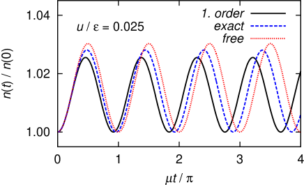
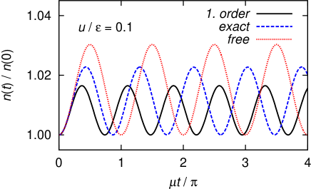
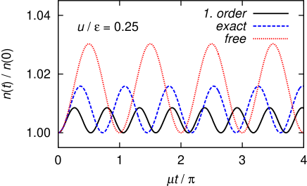
Figure 1: (Color online) Time evolution of the diagonal distribution function for initial conditions $n(0)=1$ and $p(0)=0$. We have chosen $|\gamma|/\epsilon=0.1$ and three different values of the interaction strength: $u/\epsilon=0.025$ (top), $u/\epsilon=0.1$ (middle), and $u/\epsilon=0.25$ (bottom). The frequency $\mu=\sqrt{\epsilon^{2}-|\gamma|^{2}}$ determines the oscillation period in the non-interacting limit. We compare the result of the self-consistent Hartree-Fock approximation (solid line) with the exact solution (dashed line) and the time evolution in the non-interacting limit (dotted line).

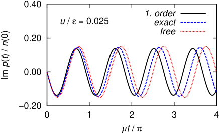
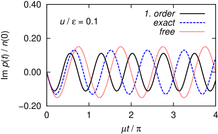
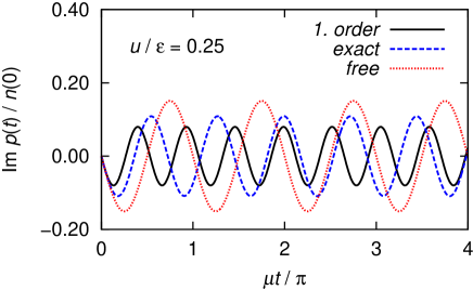
Figure 2: (Color online) Time evolution of the off-diagonal distribution function for increasing interaction strength (from top to bottom). The parameters and initial conditions are the same as in Fig. 1. We compare the result of the self-consistent Hartree-Fock approximation (solid line) with the exact solution (dashed line) and the time evolution in the non-interacting limit (dotted line).

Because our simple toy model does not account for damping and dissipative effects, the time evolution is purely oscillatory. However, the true oscillation period lies between the non-interacting oscillation period $T_{0}=\pi/\mu=\pi/\sqrt{\epsilon^{2}-|\gamma|^{2}}$ and the smaller oscillation period predicted by the self-consistent Hartree-Fock approximation. A similar phenomenon is also observed for the oscillation amplitudes. As expected the deviation between the three curves increases with increasing interaction strength. We thus conclude that the Hartree-Fock approximation is only capable for moderate interaction strength and short times as illustrated in the middle panel of Figs. 1 and 2. In this case the Hartree-Fock result up to times of the order $T_{0}/4$ is reliable. However, in this regime the free time evolution is also fairly accurate.

V.2 Kinetic equation with self-energy up to second order

Let us consider again the quantum kinetic equation for the Keldysh Green function $G^{K}(t,t^{\prime})$, which for our toy model can be obtained by simply omitting the momentum label in Eqs. (98) and (99). Substituting on the right-hand side of this equation the self-energies up to second order in the interaction given in Eq. (158) (first order self-energy) and in appendix C (second order self-energy), we obtain an equation of motion for the two-time Keldysh Green function $G^{K}(t,t^{\prime})$. Together with the corresponding retarded and advanced components of the Dyson equation, this equation forms a closed system of partial differential equations, which can in principle be solved numerically. To simplify the numerics, we will focus here only on the evolution equation for the equal-time Keldysh Green function $G^{K}(t,t)$ which can be obtained from the kinetic equation (110) by omitting the momentum labels,

$$i\partial_{t}G^{K}(t,t) - MG^{K}(t,t)-G^{K}(t,t)M^{T}$$ (172)

$$= \int_{t_{0}}^{t}dt_{1}[{Z}\Sigma^{K}(t,t_{1})G^{A}(t_{1},t)$$

$$\hskip 25.60747pt-G^{R}(t,t_{1})\Sigma^{K}(t_{1},t){Z}]$$

$$+ \int_{t_{0}}^{t}dt_{1}[{Z}\Sigma^{R}(t,t_{1})G^{K}(t_{1},t)$$

$$\hskip 25.60747pt-G^{K}(t,t_{1})\Sigma^{A}(t_{1},t){Z}].\hskip 25.60747pt$$

Since the two-time function $G^{K}(t,t^{\prime})$ appears again on the right hand side of this equation let us make three additional standard approximations to close the system of equations:

1. Generalized Kadanoff-Baym ansatz: As discussed in Sec. III.2, with the help of the generalized Kadanoff-Baym ansatz (111) we may derive a closed integral equation for the equal-time Keldysh Green function $G^{K}(t,t)$. For our toy model, the generalized Kadanoff-Baym ansatz reads

   $$G^{K}(t,t^{\prime}) \approx -i[G^{R}(t,t^{\prime})ZG^{K}(t^{\prime},t^{\prime})$$ (173)

   $$\hskip 5.69054pt-G^{K}(t,t)ZG^{A}(t,t^{\prime})].$$

   This ansatz amounts to approximating the distribution matrix in the collision integrals by its diagonal elements,

   $$[\hat{F}]_{tt^{\prime}}\equiv F(t,t^{\prime}) \approx \delta(t-t^{\prime})F(t)$$ (174)

   $$= \delta(t-t^{\prime})iZG^{K}(t,t)Z.$$

2. Markov approximation: To reduce the integro-differential equation for the equal-time Keldysh Green function to an ordinary differential equation, we replace under the integral

   $$\int_{t_{0}}^{t}dt_{1}G^{K}(t_{1},t_{1})\ldots \rightarrow G^{K}(t,t)\int_{t_{0}}^{t}dt_{1}\ldots.$$ (175)

3. Free advanced and retarded propagators: Finally, we neglect the self-energy corrections of the advanced and retarded propagators in Eq. (172) and thus replace $G^{R}(t,t^{\prime})$ and $G^{A}(t,t^{\prime})$ by the free propagators, which can be obtained by omitting the momentum labels in Eqs. (68,73).

After these approximations, the collision integrals in Eq. (172) can be calculated analytically and the non-equilibrium distribution functions are easily obtained by numerically solving a system of two coupled ordinary differential equations. For the numerical solution, the time grid was chosen equally spaced with $\Delta t\,\epsilon=1.3\times 10^{-2}$ and the differential equations were solved using a fourth-order Runge-Kutta algorithm. Hanke-Bourgeois (2006)

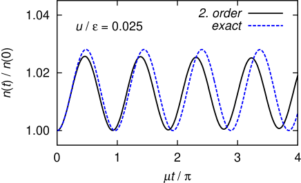
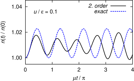
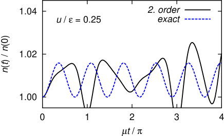
Figure 3: (Color online) Time evolution of the diagonal distribution function of the toy model. The parameters and initial conditions are the same as in Fig. 1. The solid line is the solution of the kinetic equation with second order self-energies, simplified using the generalized Kadanoff-Baym ansatz and the Markov approximation. For comparison we also show the exact solution (dashed line).

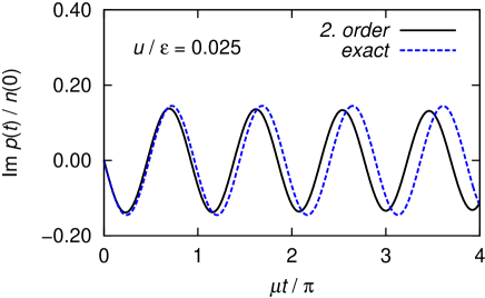
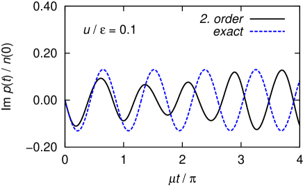
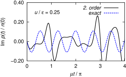
Figure 4: (Color online) Time evolution of the off-diagonal distribution function for increasing interaction strength (from top to bottom) of the toy model. The parameters and initial conditions are the same as in Fig. 1. The solid line is the solution of the kinetic equation with second order self-energies, simplified using the generalized Kadanoff-Baym ansatz and the Markov approximation. The dashed line is again the exact solution.

The result for the same parameters and initial conditions as in Figs. 1 and 2 is shown in Figs. 3 and 4. Obviously, for moderate interaction strength the inclusion of second-order corrections indeed improves the agreement with the exact solution up to times of order $T_{0}=\pi/\mu=\pi/\sqrt{\epsilon^{2}-|\gamma|^{2}}$. However, for stronger interactions and for times exceeding $T_{0}$, the solution of the kinetic equation with second-order corrections to the self-energy disagrees even more drastically from the exact solution than the time-dependent Hartree-Fock approximation shown in Figs. 1 and 2. In addition we found secular behavior and unphysical divergences of the pair correlators for long times (not shown in Figs. 3 and 4). By numerically solving the kinetic equation without making the above approximations (see appendix D), we have checked that the strong disagreement of the time evolution beyond one oscillation period $T_{0}$ with the exact result is not an artifact of the Kadanoff-Baym ansatz, the Markov approximation or the neglected renormalization of the retarded and advanced propagators.

V.3 First order truncation of the FRG hierarchy

We now show that a very simple truncation of the non-equilibrium FRG flow equation for the self-energy where the flow of the effective interaction is neglected leads to much better results for the time evolution than the previous two approximations. A similar truncation has also been made by Gezzi et al.Gezzi et al. (2007) in their FRG study of stationary non-equilibrium states of the Anderson impurity model. In the exact FRG flow equation (119) for the self-energy we replace the flowing effective interaction by the bare interaction (recall that for our toy model the collective labels $\alpha_{i}$ represents $(t_{i},\lambda_{i},\sigma_{i})$),

$$\Gamma^{(4)}_{\Lambda,\alpha_{1}\alpha_{2}\alpha_{3}\alpha_{4}}\approx\delta(t_{1}-t_{2})\delta(t_{2}-t_{3})\delta(t_{3}-t_{4})U^{\lambda_{1}\lambda_{2}\lambda_{3}\lambda_{4}}_{\sigma_{1}\sigma_{2}\sigma_{3}\sigma_{4}},$$ (176)

where up to permutation of the indices the symmetrized bare interaction is given by (see Eq. (64))

$$U_{\;\bar{a}\,\bar{a}\,a\,a}^{CQCC}=U_{\;\bar{a}\,\bar{a}\,a\,a}^{CQQQ}=U_{\;\bar{a}\,\bar{a}\,a\,a}^{CCCQ}=U_{\;\bar{a}\,\bar{a}\,a\,a}^{QQCQ}=u.\hskip 19.91692pt$$ (177)

In this approximation the two-point function is time-diagonal,

$$\Gamma^{(2)\lambda\lambda^{\prime}}_{\Lambda,\sigma t\,\sigma^{\prime}t^{\prime}}=\delta(t-t^{\prime})\Sigma^{\lambda\lambda^{\prime}}_{\Lambda,\sigma\sigma^{\prime}}(t),$$ (178)

where the self-energies satisfy the FRG flow equation

$$\partial_{\Lambda}\Sigma^{\lambda\lambda^{\prime}}_{\Lambda,\sigma\sigma^{\prime}}(t)=\frac{i}{2}\sum_{\lambda_{1}\sigma_{1}}\sum_{\lambda_{2}\sigma_{2}}U^{\lambda\lambda^{\prime}\lambda_{1}\lambda_{2}}_{\sigma\sigma^{\prime}\sigma_{1}\sigma_{2}}\dot{{G}}_{\Lambda,\sigma_{1}\sigma_{2}}^{\lambda_{1}\lambda_{2}}(t,t).$$ (179)

With the bare interaction given by Eq. (177), this leads to the FRG flow equations for the retarded ($\lambda\lambda^{\prime}=QC$) and advanced ($\lambda\lambda^{\prime}=CQ$) self-energies,

$$\partial_{\Lambda}\Sigma^{R}_{\Lambda}(t) =\partial_{\Lambda}\Sigma^{A}_{\Lambda}(t)\equiv\partial_{\Lambda}\Sigma_{\Lambda}(t)$$

$$=iu\left(\begin{array}[]{cc}\frac{1}{2}\dot{G}^{K}_{\Lambda,\bar{a}\bar{a}}(t,t)&\dot{G}^{K}_{\Lambda,a\bar{a}}(t,t)\\ \dot{G}^{K}_{\Lambda,\bar{a}a}(t,t)&\frac{1}{2}\dot{G}^{K}_{\Lambda,{a}{a}}(t,t)\end{array}\right).$$ (182)

For the Keldysh component of the self-energy corresponding to $\lambda\lambda^{\prime}=QQ$ we obtain

$$\partial_{\Lambda}\Sigma^{K}_{\Lambda,a\bar{a}}(t) =iu\left[\dot{G}^{R}_{\Lambda,a\bar{a}}(t,t)+\dot{G}^{A}_{\Lambda,a\bar{a}}(t,t)\right],$$ (183a)

$$\partial_{\Lambda}\Sigma^{K}_{\Lambda,a{a}}(t) =i\frac{u}{2}\left[\dot{G}^{R}_{\Lambda,\bar{a}\bar{a}}(t,t)+\dot{G}^{A}_{\Lambda,\bar{a}\bar{a}}(t,t)\right].$$ (183b)

From the definitions (131a,131b) of the retarded and advanced components of the single-scale propagators it is easy to see that at equal times $\dot{G}^{R}_{\Lambda}(t,t)=0=\dot{G}^{A}_{\Lambda}(t,t)$, so that within our truncation the right-hand sides of the flow-equations (183a,183b) for the Keldysh self-energy vanish. Because the initial Keldysh self-energy is zero, it remains zero during the entire RG flow within our truncation.

At this point we specify our cutoff procedure. It turns out that from the two cutoff schemes discussed in Sec. IV.2, the out-scattering rate scheme described in Sec. IV.2.2 is superior. Recall that this scheme amounts to setting $\hat{F}_{\ast,\Lambda}=0$ in Eq. (131c). For our toy model the Keldysh component of the single-scale propagator at equal times is then given by the following $2\times 2$ matrix equation,

$$\dot{G}_{\Lambda}^{K}(t,t) = i\int_{t_{0}}^{t}dt_{1}\Bigl{[}G_{\Lambda}^{R}(t,t_{1})ZG_{\Lambda}^{K}(t_{1},t)$$ (184)

$$\hskip 28.45274pt-G_{\Lambda}^{K}(t,t_{1})ZG_{\Lambda}^{A}(t_{1},t)\Bigr{]}.$$

Note that this equation still contains memory effects. We simplify Eq. (184) using the same approximations as in the previous subsection: First of all, we use the generalized Kadanoff-Baym ansatz (173) to express the Keldysh Green functions on the right-hand side of Eq. (184) in terms of the corresponding equal-time Green function. Introducing the cutoff-dependent distribution function

$$F_{\Lambda}(t)=iZG_{\Lambda}^{K}(t,t)Z,$$ (185)

we obtain

$$\dot{G}_{\Lambda}^{K}(t,t)\approx 2i\int_{t_{0}}^{t}dt_{1}G_{\Lambda}^{R}(t,t_{1})F_{\Lambda}(t_{1})G_{\Lambda}^{A}(t_{1},t).$$ (186)

Next, we replace $F_{\Lambda}(t_{1})\rightarrow F_{\Lambda}(t)$ under the integral sign (Markov approximation). Substituting the advanced and retarded propagators by their free counterparts (which can be obtained from Eq. (68,73) by omitting the momentum labels) we finally arrive at the following simple expression for the Keldysh component of the single-scale propagator in the out-scattering rate cutoff scheme,

$$\dot{G}_{\Lambda}^{K}(t,t)\approx 2i\int_{t_{0}}^{t}dt_{1}G_{0,\Lambda}^{R}(t,t_{1})F_{\Lambda}(t)G_{0,\Lambda}^{A}(t_{1},t).$$ (187)

At this point we have arrived at a system of two coupled partial differential equations (PDE) for the cutoff-dependent distribution matrix $F_{\Lambda}(t)$ and the self-energy matrix $\Sigma_{\Lambda}(t)$. The former contains the normal ($n_{\Lambda}(t)$) and anomalous ($p_{\Lambda}(t)$) distributions as in Eq. (170),

$$F_{\Lambda}(t)=\left(\begin{array}[]{cc}-2p_{\Lambda}^{\ast}(t)&2n_{\Lambda}(t)+1\\ 2n_{\Lambda}(t)+1&-2p_{\Lambda}(t)\end{array}\right).$$ (188)

The time evolution of this distribution matrix is determined by a kinetic equation which is formally identical to the corresponding kinetic equation (166) within time-dependent Hartree-Fock approximation,

$$i\partial_{t}F_{\Lambda}(t)=-M_{\Lambda}^{T}(t)F_{\Lambda}(t)-F_{\Lambda}(t)M_{\Lambda}(t).$$ (189)

The cutoff-dependent matrix $M_{\Lambda}(t)$ is

$$M_{\Lambda}(t)=M-i\Lambda I+Z\Sigma_{\Lambda}(t)$$

$$=\left(\begin{array}[]{cc}\epsilon-u-i\Lambda+\Sigma_{\Lambda,\bar{a}a}(t)&|\gamma|+\Sigma_{\Lambda,\bar{a}\bar{a}}(t)\\ -|\gamma|-\Sigma_{\Lambda,{a}{a}}(t)&-[\epsilon-u+i\Lambda+\Sigma_{\Lambda,a\bar{a}}(t)]\end{array}\right),$$ (192)

and depends on the bare matrix $M$ defined in Eq. (168), on the cutoff parameter $\Lambda$, and on the cutoff-dependent self-energy $\Sigma_{\Lambda}(t)$. The flowing self-energy matrix satisfies

$$\partial_{\Lambda}\Sigma_{\Lambda}(t)=iu\left(\begin{array}[]{cc}\frac{1}{2}\dot{G}_{\Lambda,\bar{a}\bar{a}}^{K}(t,t)&\dot{G}_{\Lambda,a\bar{a}}^{K}(t,t)\\ \dot{G}_{\Lambda,\bar{a}a}^{K}(t,t)&\frac{1}{2}\dot{G}_{\Lambda,{a}{a}}^{K}(t,t)\end{array}\right),$$ (193)

where the matrix $\dot{G}_{\Lambda}^{K}(t,t)$ is given by Eq. (187).

Mathematically, the problem is now reduced to the solution of a system of first order partial differential equations in two independent variables $t$ and $\Lambda$. To illustrate the structure more clearly, we rewrite the system (189) and (193) as

$$\partial_{t}F_{\Lambda}(t) =A(F_{\Lambda}(t),\Sigma_{\Lambda}(t),\Lambda),$$ (194a)

$$\partial_{\Lambda}\Sigma_{\Lambda}(t) =B(F_{\Lambda}(t),\Lambda,t),$$ (194b)

where the explicit form of the matrix functions $A$ and $B$ follows from the right-hand sides of Eq. (189) and (193). Note, that the system is not fully symmetric in the variables $\Lambda$ and $t$, because the flow equation contains causal memory integrals over the time $t$. Without Markov approximation, the right-hand side of the flow equation (and in higher-order truncations also the kinetic equation) is a functional of the distribution matrix $F_{\Lambda}(t)$ and depends on the distribution matrix at earlier times. Using the Markov approximation the distribution matrix can be pulled out of the integral and the functional $B$ reduces to an ordinary function of the distribution $F_{\Lambda}(t)$. To define the solution of Eqs. (194a,194b) uniquely we note that the boundary conditions fix the distribution matrix $F_{\Lambda}(t_{0})$ at the initial time $t_{0}$ and arbitrary cutoff $\Lambda$, and the self-energy matrix $\Sigma_{\Lambda_{0}}(t)$ at the initial cutoff $\Lambda_{0}$ and arbitrary time $t$. In fact, within our truncation, the boundary condition for the distribution matrix is $F_{\Lambda}(t_{0})=F(t_{0})$. Since for a large cutoff all one-particle irreducible vertices (with the exception of $\Gamma^{(4)}$) vanishes due to Eq. (138), the boundary condition for the self-energy matrix at sufficiently large initial cutoff $\Lambda_{0}$ is $\Sigma_{\Lambda_{0}}(t)=0$. The standard method of dealing with this kind of first order PDEs is the method of characteristics. *[See; forexample; ][]Zachmanoglou However, in our case the characteristic curves coincide with the curves where the boundary conditions are specified, so that the standard procedure is not applicable. Nevertheless, it is easy to see that the solution with the proper boundary conditions can be obtained by means of the following algorithm: We first note that the kinetic equation (194a) describes the propagation of $F_{\Lambda}(t)$ in $t$, and that the flow equation (194b) gives the propagation of $\Sigma_{\Lambda}(t)$ in $\Lambda$ direction, as illustrated in Fig. 5. Solving the kinetic equation (194a) for an infinitesimally small time step $dt$, the resulting distribution function at $t+dt$ can be used to integrate the flow equation (194b) at fixed $t+dt$ over $\Lambda$. Repeating these two steps allows to obtain the solution of $F_{\Lambda}(t)$ and $\Sigma_{\Lambda}(t)$ in the entire $(t,\Lambda)$-plane.

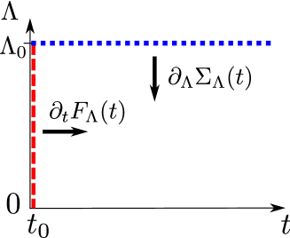
Figure 5: (Color online) Illustration of our approach to solve the system (194a) and (194b) of partial differential equations. The kinetic equation (194a) describes the propagation of $F_{\Lambda}(t)$ in $t$, where the flow equation (194b) describes the propagation of $\Sigma_{\Lambda}(t)$ in $\Lambda$-direction. The boundary conditions define the distribution function $F_{\Lambda}(t_{0})$ at the initial time $t_{0}$ (dashed line) and the self-energy $\Sigma_{\Lambda_{0}}(t)$ at the initial $\Lambda_{0}$ (dotted line).

In the following we explain our approach to numerically solve the coupled set of first order partial differential equations. We focus on the out-scattering cutoff scheme but generalizations to other cases are straightforward. We consider a discretization of the two variables $t$ and $\Lambda$ in the form

$$t\rightarrow t_{m} \in\{t_{0},\ldots,t_{M-1}\},$$ (195a)

$$\Lambda\rightarrow\Lambda_{n} \in\{\Lambda_{0},\ldots,\Lambda_{N-1}\},$$ (195b)

with $m\in\{0,\ldots,M-1\}$ and $n\in\{0,\ldots,N-1\}$. The discretized grid points are ordered as $t_{n}<t_{n+1}$ and $\Lambda_{n}>\Lambda_{n+1}$. Both grids do not need to be equally spaced. Moreover, the number of points $M$ and $N$ can be chosen arbitrarily. The discretized functions are written as

$$F_{\Lambda_{n}}(t_{m})=F_{n\,m}\quad,\quad\Sigma_{\Lambda_{n}}(t_{m})=\Sigma_{n\,m},$$ (196)

and

$$\dot{G}^{K}_{\Lambda_{n}}(t_{m},t_{m})=\dot{G}^{K}_{n\,m}.$$ (197)

The derivatives are approximated by first-order finite-difference expressions,

$$\partial_{t}F_{\Lambda_{n}}(t_{m}) \approx\frac{F_{n\,m+1}-F_{n\,m}}{t_{m+1}-t_{m}},$$ (198a)

$$\partial_{\Lambda}\Sigma_{\Lambda_{n}}(t_{m}) \approx\frac{\Sigma_{n+1\,m}-\Sigma_{n\,m}}{\Lambda_{n+1}-\Lambda_{n}}.$$ (198b)

The discretized version of the kinetic equation (166) then follows as

$$F_{n\,m+1}=F_{n\,m}+i(t_{m+1}-t_{m})(M_{n\,m}^{T}F_{n\,m}+F_{n\,m}M_{n\,m}),$$ (199)

with the time-dependent coefficient matrix

$$M_{n\,m}=M-i\Lambda_{n}I+Z\Sigma_{n\,m}.$$ (200)

In the same way the discretized flow equation (193) for the self-energy is

$$\Sigma_{n+1\,m}=\Sigma_{n\,m}$$

$$\quad+iu(\Lambda_{n+1}-\Lambda_{n})\left(\begin{array}[]{cc}\frac{1}{2}\dot{G}_{n\,m,\bar{a}\bar{a}}^{K}&\dot{G}_{n\,m,a\bar{a}}^{K}\\ \dot{G}_{n\,m,\bar{a}a}^{K}&\frac{1}{2}\dot{G}_{n\,m,{a}{a}}^{K}\end{array}\right).$$ (203)

According to Eq. (187) the single-scale propagator $\dot{G}_{n\,m}^{K}$ on the right-hand side is defined as

$$\dot{G}^{K}_{n\,m}=2i\int_{t_{0}}^{t_{m}}dt^{\prime}G^{R}_{0,\Lambda_{n}}(t_{m},t^{\prime})F_{n\,m}G^{A}_{0,\Lambda_{n}}(t^{\prime},t_{m}).$$ (204)

From the structure of the discretized equations it is obvious that causality is preserved since each time step can be calculated from the previous ones and does not depend on quantities at later times. Starting from the initial values which specify the distribution matrix $F_{n\,0}$ with $n\in\{0,\ldots,N-1\}$ and the self-energy matrix $\Sigma_{0\,m}$ with $m\in\{0,\ldots,M-1\}$ on the boundaries, one can obtain the entire solution by stepwise propagating in $t$- and in $\Lambda$-direction in terms of basic Euler steps. One Euler step from $t_{m}$ to $t_{m+1}$ contains two parts: First, with the solution $F_{n\,m}$ where $n\in\{0,\ldots,N-1\}$ from the previous step and the initial self-energy $\Sigma_{0\,m}$ on the boundary, the flow equation (V.3) at fixed time $t_{m}$ can be integrated in $N$ sub-steps from $\Lambda_{0}$ to $\Lambda_{N-1}$ to obtain $\Sigma_{n\,m}$ on all points $n\in\{0,\ldots,N-1\}$. Next, by using the kinetic equation (199), $F_{n\,m+1}$ can be derived from $F_{n\,m}$ and $\Sigma_{n\,m}$. This completes one basic Euler step since the distribution function $F_{n\,m+1}$ is now known at time $t_{m+1}$. Repeating this procedure $M$-times yields the full solution up to time $t_{M-1}$. Numerically, the first-order finite difference derivatives are not accurate enough unless the grid spacing becomes very small which is not feasible in practice. Therefore a fourth-order Runge-Kutta method for the propagation in $t$- and the second-order Heun method for the propagation in $\Lambda$-direction Hanke-Bourgeois (2006) is used. One Runge-Kutta step from $F_{n\,m}$ to $F_{n\,m+1}$ consists of four Euler steps of the form described above. The integral (204) was solved analytically using the free retarded and advanced Green functions (given by (68, 73) without $\bm{k}$ dependence). The time grid was chosen similar to the Hartree-Fock and the second-order case described in Sec. V.2. The $\Lambda$-grid ranges between $\Lambda_{0}/\epsilon=8.1$ and $\Lambda_{299}/\epsilon=2.1\times 10^{-7}$ and was adjusted in such a way that for $\Lambda/\epsilon<1$, the resolution of the grid spacing was increased to take into account the higher curvature of the self-energy in this region.

The result for the FRG approach with the out-scattering cutoff scheme for the same parameters and initial conditions as in perturbation theory (compare Figs. 1, 2 and 3, 4) is shown in Figs. 6 and 7. For the oscillation period of the pair correlators, the FRG treatment clearly improves the results compared to perturbative approaches. Up to time $T_{0}=\pi/\mu=\pi/\sqrt{\epsilon^{2}-|\gamma|^{2}}$ the period of the oscillation is nearly identical with the exact result. Even after longer times of the order $4T_{0}$ (middle panel) the deviation from the exact solution is small. The oscillation is regular and we found no secular behavior even at long times. However, the amplitude of the pair correlators is underestimated and is comparable to the perturbative mean-field result shown in Figs. 1 and 2. In contrast, with the hybridization cutoff scheme, we were not able to obtain any reasonable results for the pair-correlator dynamics. This suggests that in practice the out-scattering cutoff scheme works better than the hybridization cutoff scheme.

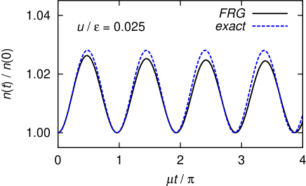
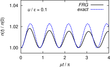
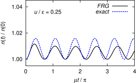
Figure 6: (Color online) The solid lines are our FRG results for the diagonal distribution function for increasing interaction strength (from top to bottom). The parameters and initial conditions are the same as in Figs. 1 and 3. For comparison we also show the exact solution (dashed line).

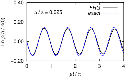
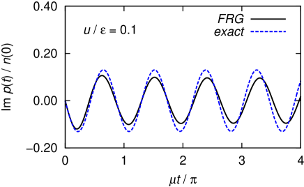
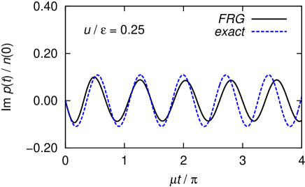
Figure 7: (Color online) The solid lines are our FRG results for the off-diagonal distribution function for increasing interaction strength (from top to bottom). The parameters and initial conditions are the same as before. The dashed line is again the exact solution.

VI Summary and conclusions

We have developed a real-time functional renormalization group (FRG) approach to calculate the time evolution of interacting bosons out of equilibrium. To be specific, we have developed our formalism in the context of the interacting time-dependent boson Hamiltonian (1) describing the non-equilibrium dynamics of magnons in dipolar magnets such as yttrium-iron garnetCherepanov et al. (1993) subject to an oscillating microwave field.Zakharov et al. (1970); L’vov (1994) To take into account the off-diagonal correlations inherent in this model we have introduced an efficient matrix notation which facilitates the derivation of quantum kinetic equations for both the normal and anomalous components of the Green functions in the Keldysh formalism. We have also extended the generalized Kadanoff-Baym ansatz Lipavský et al. (1986) to include both diagonal and off-diagonal correlations on the same footing.

In our FRG approach the time evolution of the diagonal and off-diagonal distribution functions is obtained by solving a quantum kinetic equation with cutoff-dependent collision integrals simultaneously with a renormalization group flow equation for cutoff-dependent non-equilibrium self-energies appearing in the collision integrals. To implement this procedure, we proposed a new cutoff scheme where the infinitesimal imaginary part defining the boundary conditions of the inverse advanced and retarded propagators is replaced by a finite scale acting as a running cutoff. We have called this cutoff procedure out-scattering rate cutoff scheme because the cutoff-dependent imaginary parts in the retarded and advanced propagators lead to an exponential decay of the occupation numbers. In principle one can also replace the infinitesimal imaginary part appearing in the Keldysh component of the inverse free propagator by a cutoff-dependent finite quantity which leads to the hybridization cutoff scheme proposed by Jakobs et al.. Jakobs et al. (2010b) For the toy model we presented evidence that it is better to work with the out-scattering cutoff scheme, keeping the Keldysh component of the inverse free propagator infinitesimal.

We have explicitly tested our FRG approach for a simplified toy model which is obtained from the Hamiltonian (1) by retaining only a single momentum mode. Although this simplified model does not contain damping and dissipative effects, it does describe some aspects of the magnon dynamics in yttrium-iron garnet.Kloss et al. (2010) Since the non-equilibrium time evolution of our toy model can be obtained exactly by direct numerical integration of the time-dependent Schrödinger equation, our toy model allows us to test the quality of various approximations. Specifically, we have studied the following approximations:

1. Self-consistent Hartree-Fock approximation, which is also called S-theory in the context of non-equilibrium dynamics of magnons.Zakharov et al. (1970); L’vov (1994)

2. A perturbative approach based on the calculation of the non-equilibrium self-energies to second order in the interaction, in combination with the generalized Kadanoff-Baym ansatz and the Markov approximation.

3. A FRG approach based on the simultaneous solution of a coupled system of kinetic equations and renormalization group flow equations for the scale-dependent self-energies, using a simple truncation of the FRG flow equations for the non-equilibrium self-energies where the flow of the interaction is neglected.

For each approach we have calculated the time dependence of the normal and anomalous distribution function for some representative values of the interaction and compared the result with the exact solution. It turns out that the first two approaches do not give reliable predictions for the time evolution beyond one oscillation period. Although inclusion of second order self-energy corrections somewhat improves the agreement for short times, the time dependence beyond a single oscillation period disagrees even more strongly with the exact solution than the prediction of the self-consistent Hartree-Fock approximation. In fact, in Appendix D we shall show that the numerical solution of the two-time quantum kinetic equations with second order self-energies does not lead to a better agreement with the exact solution of the toy model than calculations which in addition rely on the Kadanoff-Baym ansatz and the Markov-approximation. The perturbative approaches are therefore not able to reproduce the real-time dynamics of our toy model and do not allow for systematic improvements. The failure of perturbation theory to predict the long-time behavior of correlation functions is not unexpected.Berges (2004) In contrast, our simple truncation of the FRG flow equations in combination with the out-scattering cutoff scheme leads to quite good agreement with the exact solution over many oscillation periods. Note, however, that our FRG approach is numerically more costly than the other two methods, because one has to solve a coupled system of partial differential equations in two independent variables, the time $t$ and the cutoff-parameter $\Lambda$. Moreover, due to our simple truncation of the FRG flow equations the oscillation amplitudes are still underestimated. Nevertheless, from all approximation strategies we have tested our first order FRG approach with out-scattering cutoff scheme clearly gives the most satisfactory results for the time-evolution of our toy model. One should keep in mind, however, that the toy model does not have any intrinsic dissipation and therefore does not relax towards a stationary state at long times. In fact, we expect that for models with intrinsic dissipation other cutoff schemes such as the hybridization cutoffJakobs et al. (2010b, a) discussed in Sec. IV.2 is superior, because the hybridization cutoff retains the balance between in-scattering and out-scattering terms in the collision integral which is crucial to describe the relaxation towards a stationary state. The hybridization cutoff scheme also preserves the fluctuation-dissipation theorem during the entire flowJakobs et al. (2010a) which is advantageous close to thermal equilibrium.

Our work can be extended in several directions: First of all, it should be interesting to use our FRG approach to calculate the time evolution of infinite or open quantum systems which exhibit relaxation and dissipative processes. We expect that for such systems standard approximations such as the Kadanoff-Baym ansatz or the Markov approximation may have different regimes of validity than for our toy model. Recall that for weakly correlated systems such as semiconductors the Kadanoff Baym ansatz has been shown to be quite useful and accurate.Haug and Jauho (2008) It should also be interesting to extend our study of the toy model to the regime of strong pumping where the original vacuum state is unstable.Kloss et al. (2010) Moreover, it would be even more interesting to apply our non-perturbative FRG method to study the non-equilibrium dynamics of the time-dependent boson Hamiltonian (1) in the regime of strong pumping. It is well known Zakharov et al. (1970); L’vov (1994) that for sufficiently large values of the pumping parameter $\gamma_{\bm{k}}$ the system exhibits the phenomenon of parametric resonance. The magnon operators acquire than finite expectation values and the system approaches a non-trivial time-independent non-equilibrium state which is dominated by interactions.Zakharov et al. (1970); L’vov (1994)^,Hick et al. (2010) Although this state has been studied at the level of time-dependent Hartree-Fock approximationZakharov et al. (1970); L’vov (1994) (S-theory) it would be interesting to describe the time evolution into stationary non-equilibrium states non-perturbatively, and check if the states exhibit non-thermal scaling properties as predicted in Ref. [Berges and Hoffmeister, 2009].

APPENDIX A: TRANSFORMATION TO THE ROTATING REFERENCE FRAME

In order to simplify the calculations, it is useful to remove the explicit time-dependence from the Hamiltonian $\mathcal{H}(t)$ in Eq. (1). This can be achieved by means of a unitary transformation to the rotating reference frame, as discussed in Sec. I. In the rotating reference frame the Hamiltonian does not explicitly depend on time, see Eqs. (6). To distinguish quantities in the original- and the corresponding rotating frame, we put in this appendix an extra tilde over Green functions in the rotating frame. Introducing the unitary $2\times 2$ matrix

$$U_{\bm{k}}(t)=\left(\begin{array}[]{cc}e^{-\frac{i}{2}(\omega_{0}t-\varphi_{\bm{k}})}&0\\ 0&e^{\frac{i}{2}(\omega_{0}t-\varphi_{\bm{k}})}\end{array}\right),$$ (A1)

the relations between the elements of the matrix Green-functions $\hat{G}^{R}$, $\hat{G}^{A}$, $\hat{G}^{K}$ defined in Eqs. (16e–16o) and the corresponding quantities in the rotating reference frame (with the tilde) is

$$G^{X}(\bm{k},t,t^{\prime})=U_{\bm{k}}(t)\tilde{{G}}^{X}(\bm{k},t,t^{\prime})U_{\bm{k}}({t^{\prime}}),$$ (A2)

where $X=R,A,K$, and we have defined the $2\times 2$-matrices in flavor space,

$$G^{X}(\bm{k},t,t^{\prime})=[\hat{G}^{X}]_{\bm{k}t,-\bm{k}t^{\prime}}.$$ (A3)

Introducing the diagonal matrix

$$\hat{U}=U(t)\otimes\hat{1},$$ (A4)

with matrix elements $[\hat{U}]_{\bm{k}t,\bm{k^{\prime}}t^{\prime}}=\delta_{\bm{k},\bm{k^{\prime}}}\delta(t-t^{\prime})U_{\bm{k}}(t)$, we can rewrite Eq. (A2) in the more compact form

$$\hat{G}^{X}=\hat{U}\hat{\tilde{G}}^{X}\hat{U}.$$ (A5)

The distribution function matrix $\hat{F}$ defined via Eq. (28) is related to its counterpart $\hat{\tilde{F}}$ in the rotating reference frame via

$$\hat{F}=\hat{U}^{\dagger}\hat{\tilde{F}}\hat{U}^{\dagger}.$$ (A6)

Taking matrix elements in the time-labels and using the fact that in the non-interacting limit the distribution function matrix is time-diagonal (see Eqs. (83)), the relation (A6) implies the $2\times 2$ matrix equation,

$$F_{0}(\bm{k},t)=U^{\dagger}_{\bm{k}}(t)\tilde{F}_{0}(\bm{k},t)U^{\dagger}_{\bm{k}}(t),$$ (A7)

where we have used the fact that

$$U^{\dagger}_{\bm{k}}(t)=Z^{T}U_{\bm{k}}(t)Z=ZU_{\bm{k}}(t)Z^{T}.$$ (A8)

APPENDIX B: GENERALIZED KADANOFF-BAYM ANSATZ

The generalized Kadanoff-Baym ansatz (GKBA) is an approximate relation between matrix elements of the Keldysh Green function at different times and its equal-time counterparts. To derive the matrix form of the GKBA given in (111) formally and to identify the terms which are neglected if one uses this ansatz, we follow the derivation by Lipavský et al.. Lipavský et al. (1986) Without any loss of generality we will neglect the momentum labels for a moment and concentrate on the time dependence only. In addition we use the short-hand notation $G_{tt^{\prime}}\equiv[\hat{G}]_{tt^{\prime}}$ for the matrix elements in the time labels. We introduce

$$G^{KR}_{tt^{\prime}}=G^{KR}(t,t^{\prime}) = \Theta(t-t^{\prime})G^{K}(t,t^{\prime}),$$ (B1a)

$$G^{KA}_{tt^{\prime}}=G^{KA}(t,t^{\prime}) = \Theta(t^{\prime}-t)G^{K}(t,t^{\prime}),$$ (B1b)

so that by definition

$$G^{K}_{tt^{\prime}}=G^{KR}_{tt^{\prime}}+G^{KA}_{tt^{\prime}}.$$ (B2)

Note that the above functions are $2\times 2$ matrices in flavor space. Acting with $(\hat{G}^{R})^{-1}$ from the left on Eq. (B1a) and using the left Dyson equation (89a) for the retarded Green function we obtain

$$[(\hat{G}^{R})^{-1}\hat{G}^{KR}]_{tt^{\prime}}=-i\delta(t-t^{\prime})ZG^{K}_{tt^{\prime}}$$

$$\qquad+\Theta(t-t^{\prime})\left([(\hat{G}_{0}^{R})^{-1}\hat{G}^{K}]_{tt^{\prime}}-\int_{t^{\prime}}^{t}dt_{1}\Sigma^{R}_{tt_{1}}G^{K}_{t_{1}t^{\prime}}\right).$$ (B3)

A similar relation can be derived for the advanced component of the Keldysh Green function,

$$[\hat{G}^{KA}(\hat{G}^{A})^{-1}]_{tt^{\prime}}=i\delta(t-t^{\prime})G^{K}_{tt^{\prime}}Z$$

$$\qquad+\Theta(t^{\prime}-t)\left([\hat{G}^{K}(\hat{G}_{0}^{A})^{-1}]_{tt^{\prime}}-\int_{t}^{t^{\prime}}dt_{1}G^{K}_{tt_{1}}\Sigma^{A}_{t_{1}t^{\prime}}\right).$$ (B4)

Using the Keldysh components of the left and right Dyson equations given in Eqs. (89c) and (91c), the action of the free inverse propagators on $\hat{G}^{K}$ can be written as

$$[(\hat{G}_{0}^{R})^{-1}\hat{G}^{K}]_{tt^{\prime}}=\int_{-\infty}^{t}\!\!dt_{1}\Sigma^{R}_{tt_{1}}G^{K}_{t_{1}t^{\prime}}+\int_{-\infty}^{t^{\prime}}\!\!dt_{1}\Sigma^{K}_{tt_{1}}G^{A}_{t_{1}t^{\prime}},$$ (B5)

$$[\hat{G}^{K}(\hat{G}_{0}^{A})^{-1}]_{tt^{\prime}}=\int_{-\infty}^{t^{\prime}}\!\!dt_{1}G^{K}_{tt_{1}}\Sigma^{A}_{t_{1}t^{\prime}}+\int_{-\infty}^{t}\!\!dt_{1}G^{R}_{tt_{1}}\Sigma^{K}_{t_{1}t^{\prime}}.$$ (B6)

Substituting these expressions into Eqs. (B3) and (B4) and solving for $\hat{G}^{KR}$ and $\hat{G}^{KA}$ we obtain

$$[\hat{G}^{KR}]_{tt^{\prime}}=-iG^{R}_{tt^{\prime}}ZG^{K}_{t^{\prime}t^{\prime}}+\Theta(t-t^{\prime})$$

$$\quad\,\times\int_{t^{\prime}}^{t}dt_{1}\int_{-\infty}^{t^{\prime}}dt_{2}\,G^{R}_{tt_{1}}\left[\Sigma^{R}_{t_{1}t_{2}}G^{K}_{t_{2}t^{\prime}}+\Sigma^{K}_{t_{1}t_{2}}G^{A}_{t_{2}t^{\prime}}\right],$$ (B7)

$$[\hat{G}^{KA}]_{tt^{\prime}}=iG^{K}_{tt}ZG^{A}_{tt^{\prime}}+\Theta(t^{\prime}-t)$$

$$\quad\,\times\int^{t^{\prime}}_{t}dt_{1}\int_{-\infty}^{t}dt_{2}\left[G^{K}_{tt_{2}}\Sigma^{A}_{t_{2}t_{1}}+G^{R}_{tt_{2}}\Sigma^{K}_{t_{2}t_{1}}\right]G^{A}_{t_{1}t^{\prime}}.$$ (B8)

Adding Eqs. (B7) and (B8) we obtain the following exact integral equation for the Keldysh component of the Green function,

$$[\hat{G}^{K}]_{tt^{\prime}}=-i\left[G^{R}_{tt^{\prime}}ZG^{K}_{t^{\prime}t^{\prime}}-G^{K}_{tt}ZG^{A}_{tt^{\prime}}\right]$$

$$\quad+\Theta(t-t^{\prime})\int_{t^{\prime}}^{t}\!dt_{1}\!\!\int_{-\infty}^{t^{\prime}}\!\!\!dt_{2}\,G^{R}_{tt_{1}}\!\left[\Sigma^{R}_{t_{1}t_{2}}G^{K}_{t_{2}t^{\prime}}+\Sigma^{K}_{t_{1}t_{2}}G^{A}_{t_{2}t^{\prime}}\right]$$

$$\quad+\Theta(t^{\prime}-t)\int^{t^{\prime}}_{t}\!\!dt_{1}\!\!\int_{-\infty}^{t}\!\!\!dt_{2}\left[G^{K}_{tt_{2}}\Sigma^{A}_{t_{2}t_{1}}+G^{R}_{tt_{2}}\Sigma^{K}_{t_{2}t_{1}}\right]G^{A}_{t_{1}t^{\prime}}.$$ (B9)

To rewrite this equation in a more compact form we introduce the functions

$$W^{R}_{tt^{\prime}}=\Theta(t-t^{\prime})\int_{-\infty}^{\infty}dt_{2}(\Sigma^{R}_{tt_{2}}G^{KA}_{t_{2}t^{\prime}}+\Sigma^{K}_{tt_{2}}G^{A}_{t_{2}t^{\prime}}),$$ (B10a)

$$W^{A}_{tt^{\prime}}=\Theta(t^{\prime}-t)\int_{-\infty}^{\infty}dt_{2}(G^{KR}_{tt_{2}}\Sigma^{A}_{t_{2}t^{\prime}}+G^{R}_{tt_{2}}\Sigma^{K}_{t_{2}t^{\prime}}).$$ (B10b)

Then we may write

$$[\hat{G}^{KR}]_{tt^{\prime}} = -iG^{R}_{tt^{\prime}}ZG^{K}_{t^{\prime}t^{\prime}}+\Theta(t-t^{\prime})\int_{-\infty}^{\infty}dt_{1}G^{R}_{tt_{1}}W^{R}_{t_{1}t^{\prime}}$$ (B11)

$$= -iG^{R}_{tt^{\prime}}ZG^{K}_{t^{\prime}t^{\prime}}+\int_{-\infty}^{\infty}dt_{1}G^{R}_{tt_{1}}W^{R}_{t_{1}t^{\prime}}$$

$$= -\int_{-\infty}^{\infty}dt_{1}G^{R}_{tt_{1}}ZF^{R}_{t_{1}t^{\prime}}$$

$$= -[\hat{G}^{R}\hat{Z}\hat{F}^{R}]_{tt^{\prime}},$$

$$[\hat{G}^{KA}]_{tt^{\prime}} = iG^{K}_{tt}ZG^{A}_{tt^{\prime}}+\Theta(t^{\prime}-t)\int_{-\infty}^{\infty}dt_{1}W^{A}_{tt_{1}}G^{A}_{t_{1}t^{\prime}}$$ (B12)

$$= iG^{K}_{tt}ZG^{A}_{tt^{\prime}}+\int_{-\infty}^{\infty}dt_{1}W^{A}_{tt_{1}}G^{A}_{t_{1}t^{\prime}}$$

$$= \int_{-\infty}^{\infty}dt_{1}F^{A}_{tt_{1}}Z{G}^{A}_{t_{1}t^{\prime}}$$

$$= [\hat{F}^{A}\hat{Z}\hat{G}^{A}]_{tt^{\prime}},$$

and hence

$$\hat{G}^{K}=-\hat{G}^{R}\hat{Z}\hat{F}^{R}+\hat{F}^{A}\hat{Z}\hat{G}^{A}.$$ (B13)

Here the retarded and advanced component of the distribution function matrix is defined by

$$\hat{F}^{R} =\hat{F}^{D}+\hat{Z}\hat{W}^{R},$$ (B14a)

$$\hat{F}^{A} =\hat{F}^{D}-\hat{W}^{A}\hat{Z},$$ (B14b)

with the time-diagonal part given by

$$[\hat{F}^{D}]_{tt^{\prime}}=i\delta(t-t^{\prime})G^{K}(t,t).$$ (B15)

One easily verifies that the blocks have the following symmetries,

$$(\hat{G}^{KR})^{T} =\hat{G}^{KA},$$ (B16a)

$$(\hat{W}^{R})^{T} =\hat{W}^{A},$$ (B16b)

$$(\hat{F}^{R})^{T} =\hat{F}^{A},$$ (B16c)

$$(\hat{F}^{D})^{T} =\hat{F}^{D}.$$ (B16d)

The above relations are all exact. Comparing Eq. (28) with Eq. (B13), we conclude that the parametrization in Eq. (28) is indeed correct, and that

$$\hat{F}=\hat{Z}\hat{F}^{R}\hat{Z}.$$ (B17)

The GKBA amounts to retaining only the diagonal part $\hat{F}^{D}$ of the distribution function. Then the matrix elements of the general relation (B13) reduce to

$$G^{K}(t,t^{\prime})=-i[G^{R}(t,t^{\prime})ZG^{K}(t^{\prime},t^{\prime})-G^{K}(t,t)ZG^{A}(t,t^{\prime})].$$ (B18)

This is identical to the GKBA ansatz (173) which was used to study the toy model. Repeating the above calculation in the same fashion including the full momentum dependence leads to the relation (111).

APPENDIX C: SECOND ORDER SELF-ENERGY OF THE TOY MODEL

In this appendix we explicitly give the matrix elements of the non-equilibrium self-energies $\Sigma_{2}(t,t^{\prime})$ of our toy model introduced in Sec. V to second order in the interaction. Ignoring Hartree type of diagrams which are implicitly taken into account by imposing self-consistency in the first order calculation, the non-equilibrium self-energy to second order in the interaction is in the contour basis ($p,p^{\prime}\in\{+,-\}$) given by

$$[\hat{\Sigma}_{2}]^{pp^{\prime}}_{tt^{\prime}}=\left(\begin{array}[]{cc}\Sigma^{pp^{\prime}}_{2,aa}(t,t^{\prime})&\Sigma^{pp^{\prime}}_{2,a\bar{a}}(t,t^{\prime})\\ \Sigma^{pp^{\prime}}_{2,\bar{a}a}(t,t^{\prime})&\Sigma^{pp^{\prime}}_{2,\bar{a}\bar{a}}(t,t^{\prime})\end{array}\right)=-2u^{2}pp^{\prime}\left(\begin{array}[]{c|cc}G^{pp^{\prime}}_{aa}(G^{pp^{\prime}}_{\bar{a}\bar{a}})^{2}+2G^{pp^{\prime}}_{\bar{a}\bar{a}}G^{pp^{\prime}}_{a\bar{a}}G^{pp^{\prime}}_{\bar{a}a}&&G^{pp^{\prime}}_{a\bar{a}}(G^{pp^{\prime}}_{\bar{a}{a}})^{2}+2G^{pp^{\prime}}_{\bar{a}{a}}G^{pp^{\prime}}_{a{a}}G^{pp^{\prime}}_{\bar{a}\bar{a}}\\ \hline\cr G^{pp^{\prime}}_{\bar{a}{a}}(G^{pp^{\prime}}_{a\bar{a}})^{2}+2G^{pp^{\prime}}_{{a}\bar{a}}G^{pp^{\prime}}_{\bar{a}\bar{a}}G^{pp^{\prime}}_{{a}{a}}&&G^{pp^{\prime}}_{\bar{a}\bar{a}}(G^{pp^{\prime}}_{{a}{a}})^{2}+2G^{pp^{\prime}}_{{a}{a}}G^{pp^{\prime}}_{\bar{a}a}G^{pp^{\prime}}_{a\bar{a}}\end{array}\right),$$ (C5)

where the time labels of all Green functions are $(t,t^{\prime})$. Using the relations (47a–47c) we obtain for the normal part of the matrix elements of the self-energy in the Keldysh (RAK)-basis,

$$\Sigma^{R}_{2,a\bar{a}}(t,t^{\prime})= -\frac{u^{2}}{2}\Bigl{\{}G^{R}_{a\bar{a}}[(G^{R}_{\bar{a}a})^{2}+(G^{K}_{\bar{a}a})^{2}]+2G^{K}_{a\bar{a}}G^{R}_{\bar{a}a}G^{K}_{\bar{a}a}+2G^{R}_{\bar{a}a}[G^{R}_{aa}G^{R}_{\bar{a}\bar{a}}+G^{K}_{aa}G^{K}_{\bar{a}\bar{a}}]+2G^{K}_{\bar{a}a}[G^{R}_{aa}G^{K}_{\bar{a}\bar{a}}+G^{K}_{aa}G^{R}_{\bar{a}\bar{a}}]\Bigl{\}},$$ (C7a)

$$\Sigma^{A}_{2,a\bar{a}}(t,t^{\prime})= \left\{\mbox{replace $R\rightarrow A$ in the above expression for $\Sigma^{R}_{2,a\bar{a}}(t,t^{\prime})$ }\right\},$$ (C7b)

$$\Sigma^{K}_{2,a\bar{a}}(t,t^{\prime})= -\frac{u^{2}}{2}\Bigl{\{}G^{K}_{a\bar{a}}[(G^{R}_{\bar{a}a})^{2}+(G^{A}_{\bar{a}a})^{2}+(G^{K}_{\bar{a}a})^{2}]+2[G^{R}_{a\bar{a}}G^{R}_{\bar{a}a}+G^{A}_{a\bar{a}}G^{A}_{\bar{a}a}]G^{K}_{\bar{a}a}$$

$$+2G^{K}_{\bar{a}a}[G^{R}_{aa}G^{R}_{\bar{a}\bar{a}}+G^{A}_{aa}G^{A}_{\bar{a}\bar{a}}+G^{K}_{aa}G^{K}_{\bar{a}\bar{a}}]+2G^{R}_{\bar{a}a}[G^{K}_{aa}G^{R}_{\bar{a}\bar{a}}+G^{R}_{aa}G^{K}_{\bar{a}\bar{a}}]+2G^{A}_{\bar{a}a}[G^{K}_{aa}G^{A}_{\bar{a}\bar{a}}+G^{A}_{aa}G^{K}_{\bar{a}\bar{a}}]\Bigr{\}}$$

$$= \frac{u^{2}}{2}\Bigl{\{}G^{K}_{a\bar{a}}[(G^{I}_{\bar{a}a})^{2}-(G^{K}_{\bar{a}a})^{2}]+2G^{I}_{a\bar{a}}G^{I}_{\bar{a}a}G^{K}_{\bar{a}a}+2G^{K}_{\bar{a}a}[G^{I}_{aa}G^{I}_{\bar{a}\bar{a}}-G^{K}_{aa}G^{K}_{\bar{a}\bar{a}}]+2G^{I}_{\bar{a}a}[G^{K}_{aa}G^{I}_{\bar{a}\bar{a}}+G^{I}_{{a}a}G^{K}_{\bar{a}\bar{a}}]\Bigr{\}},$$ (C7c)

where $G^{I}_{\sigma\sigma^{\prime}}(t,t^{\prime})$ is the matrix element of the matrix $\hat{G}^{I}$ defined in Eq. (103), i.e.,

$$G^{I}_{\sigma\sigma^{\prime}}(t,t^{\prime})=i[G^{R}_{\sigma\sigma^{\prime}}(t,t^{\prime})-G^{A}_{\sigma\sigma^{\prime}}(t,t^{\prime})],$$ (C8)

and we have used the fact that $G^{R}(t,t^{\prime})G^{A}(t,t^{\prime})=0$. The corresponding self energies $\Sigma^{R}_{2,\bar{a}{a}}(t,t^{\prime})$, $\Sigma^{A}_{2,\bar{a}{a}}(t,t^{\prime})$, and $\Sigma^{K}_{2,\bar{a}{a}}(t,t^{\prime})$ can be obtained by simply exchanging $a\leftrightarrow\bar{a}$ in the above expressions. The anomalous components of the self-energy are

$$\Sigma^{R}_{2,a{a}}(t,t^{\prime})= -\frac{u^{2}}{2}\Bigl{\{}G^{R}_{a{a}}[(G^{R}_{\bar{a}\bar{a}})^{2}+(G^{K}_{\bar{a}\bar{a}})^{2}]+2G^{K}_{a{a}}G^{R}_{\bar{a}\bar{a}}G^{K}_{\bar{a}\bar{a}}+2G^{R}_{\bar{a}\bar{a}}[G^{R}_{a\bar{a}}G^{R}_{\bar{a}{a}}+G^{K}_{a\bar{a}}G^{K}_{\bar{a}{a}}]+2G^{K}_{\bar{a}\bar{a}}[G^{R}_{a\bar{a}}G^{K}_{\bar{a}{a}}+G^{K}_{a\bar{a}}G^{R}_{\bar{a}{a}}]\Bigl{\}},$$ (C9a)

$$\Sigma^{A}_{2,a{a}}(t,t^{\prime})= \left\{\mbox{replace $R\rightarrow A$ in the above expression for $\Sigma^{R}_{2,a{a}}(t,t^{\prime})$}\right\},$$ (C9b)

$$\Sigma^{K}_{2,a{a}}(t,t^{\prime})= -\frac{u^{2}}{2}\Bigl{\{}G^{K}_{a{a}}[(G^{R}_{\bar{a}\bar{a}})^{2}+(G^{A}_{\bar{a}\bar{a}})^{2}+(G^{K}_{\bar{a}\bar{a}})^{2}]+2[G^{R}_{a{a}}G^{R}_{\bar{a}\bar{a}}+G^{A}_{a{a}}G^{A}_{\bar{a}\bar{a}}]G^{K}_{\bar{a}\bar{a}}$$

$$+2G^{K}_{\bar{a}\bar{a}}[G^{R}_{a\bar{a}}G^{R}_{\bar{a}{a}}+G^{A}_{a\bar{a}}G^{A}_{\bar{a}{a}}+G^{K}_{a\bar{a}}G^{K}_{\bar{a}{a}}]+2G^{R}_{\bar{a}\bar{a}}[G^{K}_{a\bar{a}}G^{R}_{\bar{a}{a}}+G^{R}_{a\bar{a}}G^{K}_{\bar{a}a}]+2G^{A}_{\bar{a}\bar{a}}[G^{K}_{a\bar{a}}G^{A}_{\bar{a}{a}}+G^{A}_{a\bar{a}}G^{K}_{\bar{a}{a}}]\Bigr{\}}$$

$$= \frac{u^{2}}{2}\Bigl{\{}G^{K}_{a{a}}[(G^{I}_{\bar{a}\bar{a}})^{2}-(G^{K}_{\bar{a}\bar{a}})^{2}]+2G^{I}_{a{a}}G^{I}_{\bar{a}\bar{a}}G^{K}_{\bar{a}\bar{a}}+2G^{K}_{\bar{a}\bar{a}}[G^{I}_{a\bar{a}}G^{I}_{\bar{a}{a}}-G^{K}_{a\bar{a}}G^{K}_{\bar{a}{a}}]+2G^{I}_{\bar{a}\bar{a}}[G^{K}_{a\bar{a}}G^{I}_{\bar{a}{a}}+G^{I}_{{a}\bar{a}}G^{K}_{\bar{a}{a}}]\Bigr{\}}.$$ (C9c)

Finally, the conjugate anomalous self-energies $\Sigma^{R}_{2,\bar{a}\bar{a}}(t,t^{\prime})$, $\Sigma^{A}_{2,\bar{a}\bar{a}}(t,t^{\prime})$, and $\Sigma^{K}_{2,\bar{a}\bar{a}}(t,t^{\prime})$ can be obtained by exchanging $a\leftrightarrow\bar{a}$ on both sides of Eqs. (C9a-C9c). In order to calculate the “out-scattering term” (107b) in the kinetic equation, we need only the difference between retarded and advanced self-energies, which to second order in the interaction can be written as

$$\Sigma^{I}_{2,a\bar{a}}(t,t^{\prime})\equiv i[\Sigma^{R}_{2,a\bar{a}}(t,t^{\prime})-\Sigma^{A}_{2,a\bar{a}}(t,t^{\prime})] = \frac{u^{2}}{2}\Bigl{\{}G^{I}_{a\bar{a}}[(G^{I}_{\bar{a}a})^{2}-(G^{K}_{\bar{a}a})^{2}]-2G^{K}_{a\bar{a}}G^{I}_{\bar{a}a}G^{K}_{\bar{a}a}$$ (C10)

$$\hskip 14.22636pt+2G^{I}_{\bar{a}a}[G^{I}_{aa}G^{I}_{\bar{a}\bar{a}}-G^{K}_{aa}G^{K}_{\bar{a}\bar{a}}]-2G^{K}_{\bar{a}a}[G^{I}_{aa}G^{K}_{\bar{a}\bar{a}}+G^{K}_{aa}G^{I}_{\bar{a}\bar{a}}]\Bigl{\}},$$

$$\Sigma^{I}_{2,a{a}}(t,t^{\prime})\equiv i[\Sigma^{R}_{2,a{a}}(t,t^{\prime})-\Sigma^{A}_{2,a{a}}(t,t^{\prime})] = \frac{u^{2}}{2}\Bigl{\{}G^{I}_{a{a}}[(G^{I}_{\bar{a}\bar{a}})^{2}-(G^{K}_{\bar{a}\bar{a}})^{2}]-2G^{K}_{a{a}}G^{I}_{\bar{a}\bar{a}}G^{K}_{\bar{a}\bar{a}}$$ (C11)

$$\hskip 14.22636pt+2G^{I}_{\bar{a}\bar{a}}[G^{I}_{a\bar{a}}G^{I}_{\bar{a}{a}}-G^{K}_{a\bar{a}}G^{K}_{\bar{a}{a}}]-2G^{K}_{\bar{a}\bar{a}}[G^{I}_{a\bar{a}}G^{K}_{\bar{a}{a}}+G^{K}_{a\bar{a}}G^{I}_{\bar{a}{a}}]\Bigl{\}}.$$

The functions $\Sigma^{I}_{2,\bar{a}a}(t,t^{\prime})$ and $\Sigma^{I}_{2,\bar{a}\bar{a}}(t,t^{\prime})$ can again be obtained by exchanging $a\leftrightarrow\bar{a}$ in the above expressions.

APPENDIX D: SOLUTION OF THE TWO-TIME KINETIC EQUATIONS FOR THE TOY MODEL

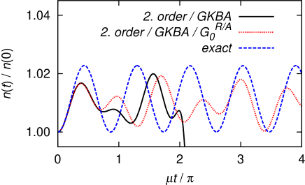
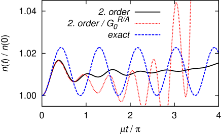
Figure 8: (Color online) Time evolution of the diagonal distribution function for the second-order self-energy without Markov approximation. We compare the result with GKBA (top) and the full two-time result without GKBA (bottom). For the retarded and advanced propagators we used the renormalized (solid line) or the free propagators (dashed line). The parameters and initial conditions are the same as in the middle panel in Fig. 1. The dashed line is again the exact solution.

In this appendix we examine the validity of the three approximations made in Sec. V.2 to obtain a closed system of equations for the equal-time Keldysh-Green function of our toy model: the Kadanoff-Baym ansatz, the Markov approximation, and the neglected renormalization of the retarded and advanced propagators. For simplicity, we focus on the kinetic equations for our toy model with the perturbative second-order self-energy. We compare different combinations of these approximations and their influence on the results. For our toy model we can obtain the quantum dynamics without relying on any of these approximations by solving the two-time quantum dynamic partial differential equations numerically. Technically, this is almost as simple as solving a system of ordinary differential equations in the equal-time formalism, except that now we have to propagate in two different time directions $t$ and $t^{\prime}$. The collision integrals were calculated numerically using the trapezoidal rule. To shorten the presentation, we will concentrate on the dynamics of the normal pair-correlator with the interaction strength $u/\epsilon=0.1$ corresponding to the middle panel in Fig. 3. The pumping strength $|\gamma|$ and the initial conditions are the same as before.

To begin with, we have solved the kinetic equation (172) for $G^{K}$ using the GKBA but without Markov approximation. The results are shown in the upper panel of Fig. 8 where we compare two different variants, depending how the retarded and advanced Green functions entering the collision integral in Eq. (172) are handled. In the first case we solved the kinetic equation (172) for $G^{K}$ together with the equations for the renormalized retarded and the advanced Green functions, which can be obtained from Eq. (97) by simply omitting the momentum labels. The set of kinetic equations was solved self-consistently using only the GKBA in the collision integrals. This combination turned out to be quite unstable and the solutions of the equations diverge slightly above the time $\mu t/\pi=2$. We have checked that the divergence is not an artifact of our grid discretization. In the second case we used the free retarded and advanced Green functions in the collision integral of the kinetic equation (172). The solution is again stable but shows an irregular dynamics in comparison with the exact solution. Compared to the analogous results relying in addition on the Markov approximation shown in Fig. 3 we did not find any improvement.

Next, we additionally avoided the GKBA. In the lower panel of Fig. 8 we compare the two different variants using the full renormalized or the free retarded and advanced propagators in the collision integral. In the first case with the full renormalized quantities, the set of kinetic equations (97,98,99) without momentum labels was solved simultaneously. The dynamics is stable, but the oscillation amplitude disappears nearly completely. In the variant with the free advanced and retarded Green functions the dynamics changes completely and the solution shows large oscillations of the pair-correlator amplitude. Again we do not observe any improvements towards the correct solution.

In summary, despite the known limitations of the GKBA and the Markov approximations, we have not found any improvements in the full two-time approach. Note that a similar comparison of the GKBA with full and free propagators, respectively, was performed for semiconductors in Ref. [Kwong et al., 1998], with the conclusion that the full GKBA performs rather well. At this point it is not clear to us if the different behavior in the present paper is due to a breakdown of standard perturbation theory or simply a special feature of the toy model, which contains no intrinsic dissipation.

References

• Schwinger (1961) J. Schwinger, J. Math. Phys. 2, 407 (1961).
• Bakshi and Mahanthappa (1963a) P. M. Bakshi and K. T. Mahanthappa, J. Math. Phys. 4, 1 (1963a).
• Bakshi and Mahanthappa (1963b) P. M. Bakshi and K. T. Mahanthappa, J. Math. Phys. 4, 12 (1963b).
• Kadanoff and Baym (1962) L. P. Kadanoff and G. A. Baym, Quantum Statistical Mechanics (Benjamin, New York, 1962).
• Keldysh (1964) L. V. Keldysh, Zh. Eksp. Teor. Fiz. 47, 1515 (1964), [Sov. Phys. JETP 20, 1018, (1965)].
• Rammer (2007) J. Rammer, Quantum Field Theory of Non-Equilibrium States (Cambridge University Press, Cambridge, 2007).
• Haug and Jauho (2008) H. Haug and A. P. Jauho, Quantum Kinetics in Transport and Optics of Semiconductors, 2nd ed. (Springer, Berlin, 2008).
• Kamenev (2004) A. Kamenev, in Les Houches, Volume Session LX, edited by H. Bouchiat, Y. Gefen, S. Guéron, G. Montambaux, and J. Dalibard (Elsevier, North-Holland, Amsterdam, 2004).
• Bon (2010) For recent reviews see for example, Progress in Nonequilibrium Green’s Functions IV, edited by M. Bonitz and K. Balzer (J. Phys. Conf. Ser., vol 220, 2010).
• Berges et al. (2008) J. Berges, A. Rothkopf,  and J. Schmidt, Phys. Rev. Lett. 101, 041603 (2008).
• Berges and Hoffmeister (2009) J. Berges and G. Hoffmeister, Nucl. Phys. B 813, 383 (2009).
• Berges (2002) J. Berges, Nucl. Phys. A 699, 847 (2002).
• Aarts et al. (2002) G. Aarts, D. Ahrensmeier, R. Baier, J. Berges,  and J. Serreau, Phys. Rev. D 66, 045008 (2002).
• Berges (2004) J. Berges, AIP Conf. Proc. 739, 3 (2004).
• Berges and Gasenzer (2007) J. Berges and T. Gasenzer, Phys. Rev. A 76, 033604 (2007).
• Goldenfeld (1992) N. Goldenfeld, Lectures on Phase Transitions and the Renormalization Group (Addison-Wesley, Reading, 1992).
• Mitra et al. (2006) A. Mitra, S. Takei, Y. B. Kim,  and A. J. Millis, Phys. Rev. Lett. 97, 236808 (2006).
• Takei et al. (2010) S. Takei, W. Witczak-Krempa,  and Y. B. Kim, Phys. Rev. B 81, 125430 (2010).
• Anders and Schiller (2005) F. B. Anders and A. Schiller, Phys. Rev. Lett. 95, 196801 (2005).
• Schmitteckert (2004) P. Schmitteckert, Phys. Rev. B 70, 121302 (2004).
• Schoeller (2000) H. Schoeller, Lect. Notes Phys. 544, 137 (2000).
• Keil and Schoeller (2001) M. Keil and H. Schoeller, Phys. Rev. B 63, 180302 (2001).
• Hackl and Kehrein (2009) A. Hackl and S. Kehrein, J. Phys.: Condens. Matter 21, 015601 (2009).
• Moeckel and Kehrein (2009) M. Moeckel and S. Kehrein, Annals of Physics 324, 2146 (2009).
• Canet et al. (2004) L. Canet, B. Delamotte, O. Deloubrière,  and N. Wschebor, Phys. Rev. Lett. 92, 195703 (2004).
• Canet and Chaté (2007) L. Canet and H. Chaté, J. Phys. A: Math. Theor. 40, 1937 (2007).
• Canet et al. (2010) L. Canet, H. Chaté, B. Delamotte,  and N. Wschebor, Phys. Rev. Lett. 104, 150601 (2010).
• Gezzi et al. (2007) R. Gezzi, T. Pruschke,  and V. Meden, Phys. Rev. B 75, 045324 (2007).
• Jakobs et al. (2007) S. G. Jakobs, V. Meden,  and H. Schoeller, Phys. Rev. Lett. 99, 150603 (2007).
• Jakobs et al. (2010a) S. G. Jakobs, M. Pletyukhov,  and H. Schoeller, Phys. Rev. B 81, 195109 (2010a).
• Karrasch et al. (2010a) C. Karrasch, M. Pletyukhov, L. Borda,  and V. Meden, Phys. Rev. B 81, 125122 (2010a).
• Jakobs (2009) S. G. Jakobs, Functional Renormalization Group Studies of Quantum Transport through Mesoscopic Systems, Ph.D. thesis, RWTH Aachen, Germany (2009).
• Karrasch (2010) C. Karrasch, The Functional Renormalization Group for Zero-Dimensional Quantum Systems In and Out of Equilibrium, Ph.D. thesis, RWTH Aachen, Germany (2010).
• Schoeller (2009) H. Schoeller, Eur. Phys. J. Special Topics 168, 179 (2009).
• Pletyukhov et al. (2010) M. Pletyukhov, D. Schuricht,  and H. Schoeller, Phys. Rev. Lett. 104, 106801 (2010).
• Karrasch et al. (2010b) C. Karrasch, S. Andergassen, M. Pletyukhov, D. Schuricht, L. Borda, V. Meden,  and H. Schoeller, Europhys. Lett. 90, 30003 (2010b).
• Gasenzer and Pawlowski (2008) T. Gasenzer and J. M. Pawlowski, Phys. Lett. B 670, 135 (2008).
• Gasenzer et al. (2010) T. Gasenzer, Keßler, Stefan,  and J. Pawlowski, Eur. Phys. J. C 70, 423 (2010).
• Jakobs et al. (2010b) S. G. Jakobs, M. Pletyukhov,  and H. Schoeller, J. Phys. A: Math. Theor. 43, 103001 (2010b).
• Kopietz et al. (2010) P. Kopietz, L. Bartosch,  and F. Schütz, Introduction to the Functional Renormalization Group (Springer, Berlin, 2010).
• Zakharov et al. (1970) V. E. Zakharov, V. S. L’vov,  and S. S. Starobinets, Zh. Eksp. Teor. Fiz. 59, 1200 (1970), [Sov. Phys. JETP 32, 656 (1971)].
• Zakharov et al. (1974) V. E. Zakharov, V. S. L’vov,  and S. S. Starobinets, Usp. Fiz. Nauk 114, 609 (1974), [Sov. Phys.-Usp. 17, 896 (1975)].
• L’vov (1994) V. S. L’vov, Wave Turbulence Under Parametric Excitation (Springer, New York, 1994).
• Cherepanov et al. (1993) V. Cherepanov, I. Kolokolov,  and V. L’vov, Phys. Rep. 229, 81 (1993).
• Bennemann and Ketterson (2008) K.-H. Bennemann and J. B. Ketterson, Superconductivity (Springer, Berlin, 2008).
• Note (1) Our notation is as follows: large bold-face letters such as $\mathbf{G}$ and $\mathbf{I}$ denote matrices in all labels: Keldysh labels $\lambda=C,Q$, field-type labels $\sigma=a,\mathaccentV{bar}016{a}$ (which we call flavor labels), as well as momentum and time labels. If we take matrix elements of $\mathbf{G}$ in Keldysh space the corresponding sub-blocks are denoted by capital letters with a hat, such as $\mathaccentV{hat}05E{G}^{R}$, $\mathaccentV{hat}05E{G}^{A}$, $\mathaccentV{hat}05E{G}^{K}$ and $\mathaccentV{hat}05E{I}$. If we further specify the flavor labels the resulting infinite matrices in the momentum- and time labels are denoted by small letters with a hat, such as $\mathaccentV{hat}05E{g}^{R}$ and $\mathaccentV{hat}05E{p}^{R}$ and $\mathaccentV{hat}05E{1}$, as defined in Eq. (16e). The matrix-elements of these sub-blocks in the momentum- and time labels are the Green functions defined in Eqs. (11a12c), i.e. $[\mathaccentV{hat}05E{g}^{R}]_{\bm{k}t,\bm{k}^{\prime}t^{\prime}}=\delta_{\bm{k},-\bm{k}^{\prime}}g^{R}_{\bm{k}}(t,t^{\prime})$ and $[\mathaccentV{hat}05E{p}^{R}]_{\bm{k}t,\bm{k}^{\prime}t^{\prime}}=\delta_{\bm{k},-\bm{k}^{\prime}}p^{R}_{\bm{k}}(t,t^{\prime})$. On the other hand, if we take matrix-elements of $\mathaccentV{hat}05E{G}^{R}$ in the momentum- and time labels we obtain $2\times 2$-matrices in flavor space, $[\mathaccentV{hat}05E{G}^{R}]_{\bm{k}t,\bm{k}^{\prime}t^{\prime}}=\delta_{\bm{k},-\bm{k}^{\prime}}G^{R}(\bm{k},t,t^{\prime})$ whose matrix elements consist of the functions $g^{R}_{\bm{k}}(t,t^{\prime})$, $p^{R}_{\bm{k}}(t,t^{\prime})$ and their complex conjugates, as defined in Eqs. (16e16o). In general, $2\times 2$ matrices in flavor space are denoted by capital letters such as $G,Z,M$.
• Vasiliev (1998) A. N. Vasiliev, Functional Methods in Quantum Field Theory and Statistical Physics (Gordon and Breach, Sidney, 1998).
• Schütz et al. (2005) F. Schütz, L. Bartosch,  and P. Kopietz, Phys. Rev. B 72, 035107 (2005).
• Danielewicz (1984) P. Danielewicz, Ann. Phys. 152, 239 (1984).
• Semkat et al. (2000) D. Semkat, D. Kremp,  and M. Bonitz, J. Math. Phys. 41, 7458 (2000).
• Garny and Müller (2009) M. Garny and M. M. Müller, Phys. Rev. D 80, 085011 (2009).
• Kwong and Bonitz (2000) N.-H. Kwong and M. Bonitz, Phys. Rev. Lett. 84, 1768 (2000).
• Note (2) Recall that we work in the rotating reference frame and have redefined $\mathaccentV{tilde}07E{\epsilon}_{\bm{k}}\equiv\epsilon_{\bm{k}}-\frac{\omega_{0}}{2}\rightarrow\epsilon_{\bm{k}}$ and removed the phase of $\gamma_{\bm{k}}$. In the original frame the matrix $M_{\bm{k}}$ in Eq. (55) should be replaced by the matrix
$$M_{\bm{k}}(t)=\left(\begin{array}[]{cc}\epsilon_{\bm{k}}&\gamma_{\bm{k}}e^{-i\omega_{0}t}\\ -\gamma^{\ast}_{\bm{k}}e^{i\omega_{0}t}&-\epsilon_{\bm{k}}\end{array}\right),$$
which depends explicitly on time.
• Gollisch and Wetterich (2001) T. Gollisch and C. Wetterich, Phys. Rev. Lett. 86, 1 (2001).
• Kreisel et al. (2008) A. Kreisel, F. Sauli, N. Hasselmann,  and P. Kopietz, Phys. Rev. B 78, 035127 (2008).
• Kwong et al. (1998) N. H. Kwong, M. Bonitz, R. Binder,  and H. S. Köhler, Phys. Stat. Sol. (b) 206, 197 (1998).
• Lipavský et al. (1986) P. Lipavský, V. Špička,  and B. Velický, Phys. Rev. B 34, 6933 (1986).
• Fricke (1996) J. Fricke, Transportgleichungen für quantenmechanische Vielteilchensysteme (Cuvillier Verlag, Göttingen, 1996).
• Bagnuls and Bervillier (2001) C. Bagnuls and C. Bervillier, Phys. Rep. 348, 91 (2001).
• Berges et al. (2002) J. Berges, N. Tetradis,  and C. Wetterich, Phys. Rep.  363, 223 (2002).
• Pawlowski (2007) J. M. Pawlowski, Ann. Phys. 322, 2831 (2007).
• Delamotte (2007) B. Delamotte, cond-mat/0702365 .
• Rosten (2010) O. J. Rosten, arXiv:1003.1366 [hep-th] .
• Wetterich (1993) C. Wetterich, Phys. Lett. B 301, 90 (1993).
• Schütz and Kopietz (2006) F. Schütz and P. Kopietz, J. Phys. A: Math. Gen. 39, 8205 (2006).
• Note (3) As pointed out in Refs. [\rev@citealpnumKopietz10,\tmspace+.1667em\rev@citealpnumSchuetz06], in equilibrium it is convenient to choose the cutoff-dependent Gaussian propagator such that $\mathbf{G}_{0,\Lambda}^{-1}\Phi^{0}=0$ and $[\partial_{\Lambda}\mathbf{G}_{0,\Lambda}^{-1}]\Phi^{0}=0$ which may be achieved by introducing suitable counter terms. Then the flow equation (122) for the order parameter $\Phi^{0}$ reduces to
\ilimits@β(ΛΦβ0)ΓΛ,βα(2)=i2\ilimits@β1\ilimits@β2[\mathaccentVdot05F𝐆Λ]β1β2ΓΛ,β2β1α(3).subscript\ilimits@𝛽subscriptΛsubscriptsuperscriptΦ0𝛽subscriptsuperscriptΓ2Λ𝛽𝛼𝑖2subscript\ilimits@subscript𝛽1subscript\ilimits@subscript𝛽2subscriptdelimited-[]\mathaccentV𝑑𝑜𝑡05𝐹subscript𝐆Λsubscript𝛽1subscript𝛽2subscriptsuperscriptΓ3Λsubscript𝛽2subscript𝛽1𝛼-\intop\ilimits@_{\beta}(\partial_{\Lambda}\Phi^{0}_{\beta})\Gamma^{(2)}_{\Lambda,\beta\alpha}=\frac{i}{2}\intop\ilimits@_{\beta_{1}}\intop\ilimits@_{\beta_{2}}[\mathaccentV{dot}05F{\mathbf{G}}_{\Lambda}]_{\beta_{1}\beta_{2}}\Gamma^{(3)}_{\Lambda,\beta_{2}\beta_{1}\alpha}.
Out of equilibrium the conditions $\mathbf{G}_{0,\Lambda}^{-1}\Phi^{0}=0$ and $[\partial_{\Lambda}\mathbf{G}_{0,\Lambda}^{-1}]\Phi^{0}=0$ are not satisfied for our cutoff choice, so that we have to work with the more general order parameter flow equation (122).
• Kloss et al. (2010) T. Kloss, A. Kreisel,  and P. Kopietz, Phys. Rev. B 81, 104308 (2010).
• Hanke-Bourgeois (2006) M. Hanke-Bourgeois, Grundlagen der Numerischen Mathematik und des wissenschaftlichen Rechnens (Teubner, Wiesbaden, 2006).
• Zachmanoglou and Thoe (1986) E. C. Zachmanoglou and D. W. Thoe, Introduction to Partial Differential Equations with Applications (Dover, New York, 1986).
• Hick et al. (2010) J. Hick, F. Sauli, A. Kreisel,  and P. Kopietz, Eur. Phys. J. B 78, 429 (2010).