A Droplet within the Spherical Model.
A.E. Patrick111Laboratory of Theoretical Physics, Joint Institute for Nuclear Research, Dubna 141980, Russia e-mail: patrick@theor.jinr.ru

  •   Abstract. Various substances in the liquid state tend to form droplets. In this paper the shape of such droplets is investigated within the spherical model of a lattice gas. We show that in this case the droplet boundary is always diffusive, as opposed to sharp, and find the corresponding density profiles (droplet shapes). Translation-invariant versions of the spherical model do not fix the spatial location of the droplet, hence lead to mixed phases. To obtain pure macroscopic states (which describe localized droplets) we use generalized quasi-averaging. Conventional quasi-averaging deforms droplets and, hence, can not be used for this purpose. On the contrary, application of the generalized method of quasi-averages yields droplet shapes which do not depend on the magnitude of the applied external field.
      key words: Droplet shape; lattice gas; pure phases; quasi-averages.

1 Introduction.

The purpose of the Gibbs distribution and the statistical physics in general is to provide a bridge between microscopic and macroscopic phenomena. It would be a mistake though to think that the bridge is in any sense similar to one of, for instance, London bridges. The difficulties of actual “traveling” through that bridge in the case of finite-dimensional models (with $d\geq 2$) are so formidable, that a better name for the bridge might have been a labyrinth. Therefore it was not really surprising that it were mathematicians (not physicists) who actually managed to walk through a few bridges connecting microscopic interparticle interactions with macroscopic shapes of droplets of condensed matter.

In a colossal effort beginning from works of Minlos and Sinai [8, 9] it was shown that for sufficiently low temperatures typical configurations of discrete lattice models look like a macroscopic droplet of one phase surrounded by another phase. The droplet border is sharp in the macroscopic scale, that is, the magnitude of typical fluctuations of the corresponding long contour is much smaller than the linear size of the droplet. Somewhat later the exact shape of the droplet in the case of the Ising model was also found. It is given by a curve minimizing the corresponding Wulff functional. For an accurate account of all “twists and turns”, which should be dealt with in order to walk through the bridge-labyrinth connecting the shape of a macroscopic droplet with the interaction of Ising particles, see the books [4, 12].

The behaviour of continuous lattice systems is different from that of the above mentioned discrete systems, and properties of Gibbs states of, for instance, $O(n)$-models are much less understood than those of various discrete models. Fortunately, there is a continuous lattice model which macroscopic properties can be derived from the interaction of microscopic variables with only modest efforts. This model is the, so-called, spherical lattice gas [6, 11].

The authors of the paper [11] studied the equation of state of the model — the behaviour of pressure as a function of specific volume and temperature. At the time, derivation of equation of state from a microscopic interaction was an achievement on its own right. Therefore, it is not surprising that such a question as the shape of a droplet of condensed “spherical matter” was not even considered. Moreover, the spherical lattice gas with cyclic boundary conditions is a translation invariant model. Hence, the center of the droplet is uniformly distributed over the available volume, and the constant average values of microscopic variables do not reveal the droplet shape.

At nearly the same time, in the paper [1] similar phenomena related to invariance of correlation functions were termed the degeneracy of equilibrium state, and a heuristic procedure to remedy the situation — the quasi-averages — was advertised. Calculation of quasi-averages involves switching on an appropriate symmetry-breaking field of a magnitude proportional to $\varepsilon$, and switching off the field by sending $\varepsilon\downarrow 0$ after the thermodynamic limit. It is shown in the present paper that the conventional quasi-averages allow one to find the true shape of the droplet only in a fortuitous situation when the symmetry-breaking field is already similar to the droplet shape we are looking for. The field of a different shape not only fixes the location of the droplet but also deforms it unrecognizably. Nevertheless, one can say that certain tools for finding the shape of a droplet in the spherical lattice gas were available already in early sixties, but investigation of that kind can not be found in the literature.

Two decades later the dominant terminology became pure phases and mixed phases (instead of non-degenerate and degenerate equilibrium states, respectively), see, e.g., the book [7]. More importantly, a simple criterion allowing one to answer the question whether a phase is pure or mixed became widely known: a phase is pure if the covariance of microscopic dynamic variables associated with nodes $j$ and $k$ tend to zero as the distance $|j-k|$ increases. Pure phases can be obtained with a help of quasi-averages, or by using appropriate boundary conditions, or by calculating conditional distributions. Mixed phases can always be represented as linear combinations of pure phases.

Gersch and Berlin, see [6], found the (constant) expected values, covariances, and conditional expected values of microscopic variables of the spherical lattice gas. The derived covariances do not tend to 0 with the distance between the corresponding microscopic degrees of freedom, hence, the natural phase of the lattice gas is not pure. In order to obtain the droplet shape in a situation like that, it is necessary to decompose the mixed phase into pure components. However, apparently, the authors of the paper [6] did not realize that.

In the present paper we extract pure phases of the spherical lattice gas using (generalized) quasi-averages, see [2, 3]. The investigation of the properties of the pure phases shows that the droplet in the spherical lattice gas is always diffusive. That is, the boundaries of the droplet are not sharp, not even in the macroscopic scale. The constant levels of the expected values of microscopic variables look like rounded squares, although not exactly the same ones as the rounded squares describing the sharp boundaries of the droplet within the 2D Ising model of a lattice gas.

The rest of the paper is organized as follows. Section 2 contains a precise definition of the spherical lattice gas. It also contains some well known technical results for the use in the later sections. Section 3 introduces macro states and summarizes the main results of the paper. In Section 4 we calculate the distributions of microscopic random variables in the mixed phase of the spherical lattice gas. In Section 5 we use the Lagrange method to find pure macroscopic phases for the lattice gas with periodic boundary conditions at zero temperature. Section 6 is the main part of this paper. There we use the method of quasi-averages for extracting pure macroscopic phases. The results of the paper are discussed in Section 7.

2 The model and useful facts.

The spherical lattice gas is a collection of random variables $\{x_{j},j\in Z^{d}\}$ placed at sites of an integer $d$-dimensional lattice, $Z^{d}$. Every site $j\in Z^{d}$ is specified by its $d$ integer coordinates $(j_{1},j_{2},...,j_{d})$. In the present paper we consider the case $d\geq 3$.

To define the distribution of random variables at all sites of the lattice, we first specify the joint distribution for the random variables in a finite cube

$$V_{n}=\{j\in Z^{d}:1\leq j_{\nu}\leq n,\nu=1,2,...,d\/\}$$

containing $N\equiv n^{d}$ sites, and then pass to the limit $n\to\infty$. To avoid unnecessary complications we impose periodic boundary conditions in all dimensions.

It is instructive to consider also a stretched model defined on the parallelepipeds

$$\Upsilon_{n}=\{j\in Z^{d}:1\leq j_{\nu}\leq n_{\nu},\nu=1,2,...,d\/\},$$ (1)

where $n_{1}=(1+\delta)n$, $\delta>0$, and $n_{\nu}=n$, for $\nu=2,3,...,d$. Save for one side being longer than the others, the definition of the stretched model is exactly the same as that of the conventional spherical lattice gas.

The Hamiltonian.

The random variables located in the rectangle $V_{n}$ interact with each other and with the external field $\{h_{j},j\in Z^{d}\}$ via the Hamiltonian

$$H_{n}=-J\sum_{j,k\in V_{n}}T_{jk}x_{j}x_{k}-\sum_{j\in V_{n}}h_{j}x_{j},$$ (2)

where $J>0$, and $T_{jk}$ are the elements of the nearest-neighbour interaction matrix. In this paper the field $\{h_{j},j\in Z^{d}\}$ is used as a technical tool, so that, it should not necessarily be physically sensible. We let its magnitude to depend on the size of rectangle $V_{n}$:

$$h_{j}=n^{-\gamma}b_{j},\quad j\in Z^{d},$$ (3)

where the absolute values of $b_{j}$ are bounded by an independent of $n$ constant $b$.

The interaction matrix.

The elements of the interaction matrix $\widehat{T}$ describe the usual nearest neighbour interaction on a square lattice, and they are given by

$$T_{jk}=\sum_{\nu=1}^{d}J^{(\nu)}(j_{\nu},k_{\nu})\prod_{l\in\{1,2,\ldots,d\}\setminus\nu}\delta(j_{l},k_{l}),$$

where

$$\delta(j_{l},k_{l})=\left\{\begin{array}[]{cl}1,&\mbox{ if }j_{l}=k_{l},\\ 0,&\mbox{ if }j_{l}\neq k_{l},\end{array}\right.$$

is the Kronecker delta.

The coefficients $J^{(\nu)}(j_{\nu},k_{\nu})$, for $\nu=1,2,\ldots,d$, are the elements of the matrix

$$\widehat{J}=\left(\begin{array}[]{ccccccc}0&\frac{1}{2}&&&&&\frac{1}{2}\\ \frac{1}{2}&0&\frac{1}{2}&&&\mbox{\LARGE 0}&\\ &\frac{1}{2}&0&\ddots&&&\\ &&\ddots&\ddots&\ddots&&\\ &&&\ddots&0&\frac{1}{2}&\\ &\mbox{\LARGE 0}&&&\frac{1}{2}&0&\frac{1}{2}\\ \frac{1}{2}&&&&&\frac{1}{2}&0\end{array}\right).$$

The eigenvalues and orthonormal eigenvectors of the matrix $\widehat{J}$ are given by

$$\lambda_{l}=\cos\frac{2\pi(l-1)}{n},\quad l=1,2,\ldots,n,$$

and

$$\mbox{\boldmath$u$}^{(l)}=\left\{u_{m}^{(l)}=\sqrt{\frac{2}{n}}\cos\left[\frac{2\pi(l-1)(m-1)}{n}-\frac{\pi}{4}\right]\right\}_{m=1}^{n},\quad l=1,2,\ldots,n.$$

The eigenvalues of the interaction matrix $\widehat{T}$ are the sums of eigenvalues of the matrix $\widehat{J}$:

$$\Lambda_{k}=\sum_{\nu=1}^{d}\lambda_{k_{\nu}},\quad k\equiv(k_{1},k_{2},\ldots,k_{d})\in V_{n}.$$

The corresponding orthonormal eigenvectors are the products of eigenvectors of the matrix $\widehat{J}$:

$$\mbox{\boldmath$w$}^{(k)}=\left\{w_{j}^{(k)}=\prod_{\nu=1}^{d}u_{j_{\nu}}^{(k_{\nu})}\right\}_{j\in V_{n}},\quad k\equiv(k_{1},k_{2},\ldots,k_{d})\in V_{n}.$$ (4)

Note that the second-largest eigenvalue $\Lambda_{\,\rm s}\equiv d-1+\cos(2\pi/n)$ of the interaction matrix (which will play an important role below) is $2d$ times degenerate. At the same time, in the case of the stretched model the second-largest eigenvalue $\Lambda_{\,\rm s}\equiv d-1+\cos\left[\frac{2\pi}{(1+\delta)n}\right]$ is only twice degenerate.

The Gibbs distribution.

The joint distribution of the random variables $\{x_{j},j\in V_{n}\}$ is specified by the usual Gibbs density

$$p(\{x_{j},j\in V_{n}\})=\frac{e^{-\beta H_{n}}}{\Theta_{n}(\rho)},$$

with respect to the “a priori” measure

$$\mu_{n}(dx)=\delta\left(\sum_{j\in V_{n}}x_{j}-\rho N\right)\delta\left(\sum_{j\in V_{n}}x_{j}^{2}-N\right)\prod_{j\in V_{n}}dx_{j}.$$

The first delta function imposes the typical for gas models density constraint

$$\frac{1}{N}\sum_{j\in V_{n}}x_{j}=\rho,$$

the second one imposes the usual spherical constraint

$$\sum_{j\in V_{n}}x_{j}^{2}=N.$$

The normalization factor (partition function) $\Theta_{n}(\rho)$ is given by

$$\Theta_{n}(\rho)=\int_{-\infty}^{\infty}\ldots\int_{-\infty}^{\infty}e^{-\beta H_{n}}\mu_{n}(dx).$$ (5)

3 Macro states and the main results.

The usual Gibbs states provide a detailed microscopic description of a thermodynamic system. In some sense the amount of available detail is too big: there can be a macroscopically inhomogeneous structure in the thermodynamic system, but its shape can not be described within the Gibbs-state framework. In this situation an introduction of a rougher (reduced) description seems justified and useful.

We define macro states as the following continuum limit of the original lattice system. The limiting configurations are realizations of random functions defined on the $d$-dimensional rectangle $[0,1]^{d}$:

$$\{x(\gamma)\}_{\gamma\in[0,1]^{d}}\equiv\{x(\gamma_{1},\gamma_{2},\ldots,\gamma_{d})\}_{\gamma_{1},\gamma_{2},\ldots,\gamma_{d}\in[0,1]}.$$

For any $\gamma\in[0,1]^{d}$ the random variable $x(\gamma)$ is defined as the following limit in distribution

$$x(\gamma)\stackrel{{\scriptstyle d}}{{=}}\lim_{n\to\infty}x_{([\gamma_{1}n],[\gamma_{2}n],\ldots,[\gamma_{d}n])},$$

where $[y]$, is the integer part of $y$. Of course, for correctness of the above definition we need some kind of continuity in the system, so that for two sequences $j(n)$ and $k(n)$ with the same limits

$$\lim_{n\to\infty}(j_{1}(n)/n,\ldots,j_{d}(n)/n)=\lim_{n\to\infty}(k_{1}(n)/n,\ldots,k_{d}(n)/n)=(\gamma_{1},\gamma_{2},\ldots,\gamma_{d}),$$

we also have identical limits of the corresponding sequences of random variables $\{x_{j(n)}\}_{n=1}^{\infty}$ and $\{x_{k(n)}\}_{n=1}^{\infty}$. Although in discrete spin systems that kind of continuity may well be missing, we do not worry too much about that, because it should be possible to surpass this technical problem one way or another.

Thermodynamic random variables $x(\gamma)$ and $x(\delta)$ are limits of the random sequences $x_{([\gamma_{1}n],[\gamma_{2}n],\ldots,[\gamma_{d}n])}$ and $x_{([\delta_{1}n],[\delta_{2}n],\ldots,[\delta_{d}n])}$ separated by a distance of order $n$. Hence, in the continuum limit the random variables $x(\gamma)$ and $x(\delta)$ with $\gamma\neq\delta$ are independent due to the exponential/power-law decay of correlations in pure phases of high/low temperature regions. Therefore, a pure macro state is completely characterized by individual distributions

$$F_{\gamma}(y)=\lim_{n\to\infty}\mbox{ Pr}_{\,n}\left[x_{([\gamma_{1}n],[\gamma_{2}n],\ldots,[\gamma_{d}n])}\leq y\right].$$

Macro states defined above contain complete information about the microscopic individual distributions of the random variables $x_{j}$. It might be desirable to achieve further reduction of description by using, for instance, Kadanoff’s blocks in the definition of the continuum limit. That should reduce the range of limiting distribution outside the critical lines/points to just the normal distribution. Even on critical lines the asymptotic distributions of large Kadanoff’s blocks should be of quite limited variety.

The main results of the present paper obtained for the low-temperature region $\beta>\beta_{c}(\rho)$, see Eq. (9), can be stated as follows.

  1. 1.

    The expected values of the random variables $x_{j}$ in the natural state of the spherical lattice gas are translation invariant and equal to the density, $\langle x_{j}\rangle=\rho$. Their variances and covariances in the limit $n\to\infty$ are given by

    $$\mbox{Var}(x_{j})=\frac{W_{d}(d)}{2\beta J}+\frac{1-\rho^{2}}{2}\left(1-\frac{\beta_{c}}{\beta}\right)+o(1),$$
    $$\mbox{Cov}(x_{j},x_{l})=c(j,l)+(1-\rho^{2})\left(1-\frac{\beta_{c}}{\beta}\right)\frac{1}{d}\sum_{\nu=1}^{d}\cos\frac{2\pi(j_{\nu}-l_{\nu})}{n}+o(1),$$

    where $c(j,l)$ are the covariances of the microscopic variables in the ordinary spherical model, see Eq. (21).

  2. 2.

    The random variables $x_{j}$ within the stretched model admit the following representation

    $$x_{j}=\sqrt{2(1-\rho^{2})\left(1-\frac{\beta_{c}}{\beta}\right)}\sin(2\pi\!\mbox{ \boldmath$U$})+{\cal N}_{j}\left(\rho,\frac{W_{d}(d)}{2\beta J}\right),$$

    where the random variable $U$ is uniformly distributed on the interval $[0,1]$, ${\cal N}_{j}(a,b)$ are normal random variables with mean $a$ and variance $b$, and

    $$\mbox{Cov}({\cal N}_{j},{\cal N}_{l})\equiv c(j,l)\to 0\ \mbox{as dist}(j,l)\to\infty.$$
  3. 3.

    For $T=0$ the pure equilibrium states of the model (ground states) are given by

    $$x_{j}=\rho+\sqrt{2(1-\rho^{2})}\sum_{\nu=1}^{d}r_{\nu}\cos\left[\frac{2\pi(j_{\nu}-1)}{n}-\alpha_{\nu}\right],$$

    where $\alpha_{\nu}$ and $r_{\nu}$ are any constants satisfying $\alpha_{\nu}\in[0,2\pi]$ and $\sum_{\nu=1}^{d}r^{2}_{\nu}=1$.

  4. 4.

    In the presence of a symmetry-breaking field

    $$h_{j}=\left\{\begin{array}[]{cl}\varepsilon n^{-\delta},&\mbox{ if }j_{1}=1,\\ 0,&\mbox{ otherwise,}\end{array}\right.$$

    the expected values of the random variables $x_{j}$ are given by

    xjεn(1δ)/32J2ζ[1+2ζn(1+2δ)/3]j1,similar-todelimited-⟨⟩subscript𝑥𝑗𝜀superscript𝑛1𝛿32𝐽2superscript𝜁superscriptdelimited-[]12superscript𝜁superscript𝑛12𝛿3subscript𝑗1\langle x_{j}\rangle\sim\frac{\varepsilon n^{(1-\delta)/3}}{2J\sqrt{2\zeta^{*}}}\left[1+\sqrt{2\zeta^{*}}n^{-(1+2\delta)/3}\right]^{-j_{1}},

    if $0<\delta<1$ and $j_{1}\leq n/2$. In this case all condensed “spherical matter” gathers in a narrow strip around the plane where the field is applied. The shape of the droplet is clearly deformed by the field.

    If $\delta=1$ the distributions of the random variables $x_{j}$ still depend on the magnitude of the symmetry breaking field, but in the limit $n\to\infty$ they remain proper. In particular, the finite expected values of the random variables $x_{j}$ are given by Eq. (26). The droplet shape is still deformed by the field.

    If $1<\delta<d-1$, then the limiting distributions of the random variables $x_{j}$ do not depend on the magnitude of the symmetry breaking field. In particular, the expected values of the random variables $x_{j}$ are given by

    $$\langle x_{j}\rangle=\rho+\sqrt{2(1-\rho^{2})\left(1-\frac{\beta_{c}}{\beta}\right)}\cos(2\pi\gamma_{1})+o(1).$$

    The droplet shape is determined by the field (for different field types we obtain different shapes), but it is no longer deformed by the field (does not depend on $varepsilon$).

4 The mixed phase.

Main thermodynamic properties of the spherical lattice gas with cyclic boundary conditions were derived in the papers [6, 11]. Although the free energy density of the model is not sensitive to the type of boundary conditions used, more delicate properties, like the droplet shape, are. Therefore in this section we re-derive the results of the paper [6] in the case of, more realistic, periodic boundary conditions.

The calculation of free energy, expected values, and correlation functions for the spherical lattice gas is reduced, in a routine fashion, to calculation of the large-$n$ asymptotics of an integral, see [6]. Introduction of new integration variables $y_{j}$, $j\in V_{n}$ in Eq. (5) via the orthogonal transformation

$$x_{j}=\sum_{k\in V_{n}}w_{j}^{(k)}y_{k},\quad j\in V_{n},$$ (6)

where the eigenvectors $\{w_{j}^{(k)},j\in V_{n}\}$ are given by Eq. (4), diagonalises the interaction matrix. As a result, we obtain the following expression for the partition function

$$\Theta_{n}(\rho)=\int_{-\infty}^{\infty}\ldots\int_{-\infty}^{\infty}\exp\left(\beta J\sum_{k\in V_{n}}\lambda_{k}y_{k}^{2}+\beta\sum_{k\in V_{n}}\varphi_{k}y_{k}\right)\widetilde{\mu}_{n}(dy),$$

where $\varphi_{k}=\sum_{j\in V_{n}}h_{j}w_{j}^{(k)}$, and

$$\widetilde{\mu}_{n}(dy)=\delta\left(y_{(1,1,\ldots,1)}\sqrt{N}-\rho N\right)\delta\left(\sum_{j\in V_{n}}y_{j}^{2}-N\right)\prod_{j\in V_{n}}dy_{j}.$$

Integration over $y_{(1,1,\ldots,1)}$ yields

$$\Theta_{n}(\rho)=\frac{1}{\sqrt{N}}\int_{-\infty}^{\infty}\ldots\int_{-\infty}^{\infty}\exp\left(\beta Jd\rho^{2}N+\beta J{\sum_{k\in V_{n}}}^{\prime}\lambda_{k}y_{k}^{2}+\beta\rho{\sum_{j\in V_{n}}}h_{j}+\beta{\sum_{k\in V_{n}}}^{\prime}\varphi_{k}y_{k}\right)\times$$
$$\delta\left({\sum_{k\in V_{n}}}^{\prime}y_{k}^{2}-N(1-\rho^{2})\right){\prod_{k\in V_{n}}}^{\prime}dy_{k},$$

where primes indicate that summations/products do not include $k=(1,1,\ldots,1)$.

The integral representation for the delta function

$$\delta\left({\sum_{k\in V_{n}}}^{\prime}y_{k}^{2}-N(1-\rho^{2})\right)=\frac{1}{2\pi i}\int_{-i\infty}^{+i\infty}\!ds\,\exp\left[s\left(N(1-\rho^{2})-{\sum_{k\in V_{n}}}^{\prime}y_{k}^{2}\right)\right],$$

allows one to perform integration over the variables $y_{k}$. However, we can switch the order of integration over the variables $y_{k}$ and $s$ only after a shift of the integration contour for $s$ to the right. The shift must assure that the real part of the quadratic form involving the variables $y_{k}$, is negatively defined. On switching the integration order, integrating over $y_{k}$, and introducing a new integration variable $z$ via $s=\beta Jz$ one obtains

$$\Theta_{n}(\rho)=\frac{\beta J}{2\pi i\sqrt{N}}\exp\left(\beta Jd\rho^{2}N+\beta\rho{\sum_{j\in V_{n}}}h_{j}\right)\left(\frac{\pi}{\beta J}\right)^{(N-1)/2}\int_{-i\infty+c}^{+i\infty+c}\!dz\,\exp\left[N\beta\Phi_{n}(z)\right],$$ (7)

where

$$\Phi_{n}(z)=Jz(1-\rho^{2})-\frac{1}{2\beta N}{\sum_{k\in V_{n}}}^{\prime}\ln(z-\lambda_{k})+\frac{1}{4JN}{\sum_{k\in V_{n}}}^{\prime}\frac{\varphi_{k}^{2}}{z-\lambda_{k}},$$

and $c>d$ is the shift of the integration contour mentioned above.

Depending on the value of $\beta$, the large-$n$ asymptotics of the integral (7) can be found either by the saddle-point method, or by direct integration after an appropriate change of variables. The saddle point of the integrand is a solution of the equation

$$\Phi_{n}^{\prime}(z)=J(1-\rho^{2})-\frac{1}{2\beta N}{\sum_{k\in V_{n}}}^{\prime}\frac{1}{z-\lambda_{k}}-\frac{1}{4JN}{\sum_{k\in V_{n}}}^{\prime}\frac{\varphi_{k}^{2}}{(z-\lambda_{k})^{2}}=0.$$ (8)

If the field $\{h_{j},j\in Z^{d}\}$ is of the type (3), then

$$\frac{1}{N}{\sum_{k\in V_{n}}}\frac{\varphi_{k}^{2}}{(z-\lambda_{k})^{2}}\leq\frac{n^{-2\gamma}b^{2}}{(z-d)^{2}}.$$

Hence, for any $z>d$, as $n\to\infty$, the sequence of the derivatives $\Phi_{n}^{\prime}(z)$ converges to

$$\Phi^{\prime}(z)=J(1-\rho^{2})-\frac{1}{2\beta}W_{d}(z),$$

where

$$W_{d}(z)\equiv\int_{-\pi}^{\pi}\ldots\int_{-\pi}^{\pi}\frac{1}{z-\sum_{\nu=1}^{d}\cos\omega_{\nu}}\prod_{l=1}^{d}\frac{d\omega_{l}}{2\pi}<\infty$$

is the Watson function.

The function $\Phi^{\prime}(z)$ increases monotonically with $z$ on $[d,\infty)$, and the location of its zeroes depends on the dimension $d$ of the lattice. Namely, if $d=1,2$, then the function $\Phi^{\prime}(z)$ has exactly one zero on the interval $[d,\infty)$ at a point $z^{*}(\rho)>d$, for any $\beta>0$. If $d\geq 3$, then there exists a critical value

$$\beta_{c}(\rho)=\frac{1}{2J(1-\rho^{2})}W_{d}(d)$$ (9)

of the parameter $\beta$. If $\beta<\beta_{c}(\rho)$, then the function $\Phi^{\prime}(z)$ still has exactly one zero on the interval $[d,\infty)$ at a point $z^{*}>d$. While if $\beta>\beta_{c}(\rho)$, then the function $\Phi^{\prime}(z)$ is strictly positive on the interval $[d,\infty)$.

In this section our aim is to investigate the natural state of the spherical lattice gas, which, as we shall see shortly, happens to be a mixed phase. Therefore we do not utilize any symmetry-breaking perturbations and set $h_{j}=0$ for all $j\in Z^{d}$ untill Section 6.

Application of the saddle-point method to the integral (7) is fairly straightforward when there exists a saddle point $z^{*}(\rho)$ greater than $d$. In this case

$$\Phi_{n}(z^{*}(\rho))=\underbrace{J(1-\rho^{2})z^{*}(\rho)-\frac{1}{2\beta}L_{d}(z^{*}(\rho))}_{\equiv\Phi(z^{*}(\rho))}+O(e^{-n\delta}),$$

and the saddle-point method yields

$$-f_{n}\equiv\frac{1}{\beta n^{d}}\ln\Theta_{n}(\rho)=\frac{1}{2\beta}\ln\frac{\pi}{\beta J}+Jd\rho^{2}+\Phi(z^{*}(\rho))+O\left(n^{-d}\ln n\right),$$

as $n\to\infty$, where

$$L_{d}(z)=\int_{-\pi}^{\pi}\!\ldots\int_{-\pi}^{\pi}\ln\left(z-\sum_{\nu=1}^{d}\cos\omega_{\nu}\right)\prod_{l=1}^{d}\frac{d\omega_{l}}{2\pi}.$$

When $\beta\geq\beta_{c}$, the function $\Phi_{n}(z)$ still attains its minimum on the interval $(\lambda_{\rm\,s},\infty)$ at a point $z_{n}^{*}>\lambda_{\rm\,s}$, where $\lambda_{\rm\,s}=d-1+\cos\frac{2\pi}{n}$ is the second-largest eigenvalue of the interaction matrix $\widehat{T}$. However, the sequence of saddle points $z_{n}^{*}$ approaches the pole of the integrand at $z=\lambda_{\rm\,s}$, and the application of the saddle-point method becomes a bit more tricky.

To find the asymptotics of the free energy we have to introduce a new integration variable $\zeta$ via $z=\lambda_{\rm\,s}+\zeta N^{-1}$. The large-$n$ asymptotics of the sum

$$L_{d}^{(N)}\left(\lambda_{\rm\,s}+\zeta N^{-1}\right)\equiv\frac{1}{N}{\sum_{k\in V_{n}}}^{\prime}\ln\left(\lambda_{\rm\,s}+\zeta N^{-1}-\lambda_{k}\right),$$

is given by

$$L_{d}^{(N)}\left(\lambda_{\rm\,s}+\zeta N^{-1}\right)=\frac{2d\ln(\zeta/N)}{N}+\frac{1}{N}{\sum_{k\in V_{n}}}^{\prime\prime}\ln\left(\lambda_{\rm\,s}-\lambda_{k}\right)-\frac{\zeta}{N^{2}}{\sum_{k\in V_{n}}}^{\prime\prime}\frac{1}{\lambda_{\rm\,s}-\lambda_{k}}+o(N^{-1}),$$

where the double prime indicates that the summation does not include both the largest and the ($2d$-times degenerate) second-largest eigenvalues.

Hence

$$\Theta_{n}(\rho)\sim\exp\left[N\beta J(d\rho^{2}+\lambda_{\rm\,s}(1-\rho^{2}))-\frac{1}{2}{\sum_{k\in V_{n}}}^{\prime\prime}\ln\left(\lambda_{\rm\,s}-\lambda_{k}\right)\right]\times$$
$$\beta JN^{d-3/2}\left(\frac{\pi}{\beta J}\right)^{(N-1)/2}\frac{1}{2\pi i}\int_{C}\frac{e^{J[(1-\rho^{2})\beta-\beta_{c}]\zeta}}{\zeta^{d}}\,d\zeta,$$ (10)

where the integration contour $C$ runs below the negative semi-axis $(-\infty,0]-i\,0$, encircles 00 counterclockwise, and returns to $-\infty$ above the negative semi-axis $(-\infty,0]+i\,0$.

We see that the remaining integration does not contain the large parameter $N$ any longer, and calculating the residue of the integrand at $\zeta=0$ we obtain

$$\frac{1}{2\pi i}\int_{C}\frac{e^{J[(1-\rho^{2})\beta-\beta_{c}]\zeta}}{\zeta^{d}}\,d\zeta=\frac{J^{d-1}}{(d-1)!}\left[(1-\rho^{2})\beta-\beta_{c}\right]^{d-1}.$$

We can use the same method to find the joint characteristic function $\chi(t,s)$ of random variables $x_{j}$ and $x_{l}$. First, we express $\chi(t,s)\equiv\langle\exp(itx_{j}+isx_{l})\rangle_{n}$ as the following integral

$$\chi(t,s)=\frac{e^{it\rho+is\rho}}{\Theta_{n}(\rho)\sqrt{N}}\exp\left(\beta Jd\rho^{2}N+\beta\rho\sum_{j\in V_{n}}h_{j}\right)\frac{\beta J}{2\pi i}\left(\frac{\pi}{\beta J}\right)^{(N-1)/2}\times$$
$$\int_{-i\infty+c}^{+i\infty+c}\!dz\,\exp\left[N\beta\Phi_{n}(z)-{\sum_{k\in V_{n}}}^{\prime}\frac{\left(tw_{j}^{(k)}+sw_{l}^{(k)}\right)^{2}}{4\beta J(z-\lambda_{k})}+i{\sum_{k\in V_{n}}}^{\prime}\frac{\left(tw_{j}^{(k)}+sw_{l}^{(k)}\right)\varphi_{k}}{2J(z-\lambda_{k})}\right].$$ (11)

Next, introduce a new integration variable $\zeta$ via $z=\lambda_{\rm\,s}+\zeta N^{-1}$, and use the asymptotic expansion for the partition function $\Theta_{n}(\rho)$ to obtain

$$\chi(t,s)\sim\exp\left[i(t+s)\rho-\frac{t^{2}+s^{2}}{4\beta JN}{\sum_{k\in V_{n}}}^{\prime\prime}\frac{1}{\lambda_{\rm\,s}-\lambda_{k}}-\frac{ts}{2\beta J}{\sum_{k\in V_{n}}}^{\prime\prime}\frac{w_{j}^{(k)}w_{l}^{(k)}}{\lambda_{\rm\,s}-\lambda_{k}}\right]\times$$
$$\frac{(d-1)!}{2\pi i}\int_{C}\exp\left[\zeta-\frac{1-\rho^{2}}{2\,\zeta}\left(1-\frac{\beta_{c}}{\beta}\right)\left((t^{2}+s^{2})d+2\,ts\sum_{\nu=1}^{d}\cos\frac{2\pi(j_{\nu}-k_{\nu})}{n}\right)\right]\,\frac{d\zeta}{\zeta^{d}}.$$ (12)

The remaining integral can be expressed in terms of the Bessel function

$$J_{m}(x)=\frac{1}{2\pi i}\int_{C}\exp\left[\frac{x}{2}\left(\zeta-\frac{1}{\zeta}\right)\right]\,\frac{d\zeta}{\zeta^{m+1}},$$

however, calculation of the moments can be done easily by differentiation under the integral sign in Eq. (12).

Setting $s=0$ and passing to the limit $N\to\infty$ we see that the random variables $x_{j}$ of the spherical model on the infinite lattice have the common characteristic function

$$\chi(t)=\exp\left[it\rho-\frac{t^{2}}{4\beta J}W_{d}(d)\right]\frac{(d-1)!}{2\pi i}\int_{C}\exp\left[\zeta-\frac{1-\rho^{2}}{2\,\zeta}\left(1-\frac{\beta_{c}}{\beta}\right)t^{2}d\right]\,\frac{d\zeta}{\zeta^{d}}.$$ (13)

Differentiation over $t$ shows that the expected values are given by $\langle x_{j}\rangle=\rho$, and the variances are given by

$$\mbox{Var}(x_{j})=\frac{W_{d}(d)}{2\beta J}+\frac{1-\rho^{2}}{2}\left(1-\frac{\beta_{c}}{\beta}\right).$$

More importantly, differentiation of the joint characteristic function shows that

$$\mbox{Cov}(x_{j},x_{l})=(1-\rho^{2})\left(1-\frac{\beta_{c}}{\beta}\right)\frac{1}{d}\sum_{\nu=1}^{d}\cos\frac{2\pi(j_{\nu}-l_{\nu})}{n}.$$

Note that $\mbox{Cov}(x_{j},x_{l})\not\to 0$, as $\mbox{dist}(j,l)\to\infty$, for any $\beta>\beta_{c}$. Therefore, the lattice gas is in a mixed (or degenerate) state, and in order to calculate the values of observable quantities we have to single out pure phases.

In the case of the stretched lattice (1) the second-largest eigenvalue of the interaction matrix is only twice degenerate, and we obtain

$$\chi(t,s)\sim\exp\left[i(t+s)\rho-\frac{t^{2}+s^{2}}{4\beta JN}{\sum_{k\in\Upsilon_{n}}}^{\prime\prime}\frac{1}{\lambda_{\rm\,s}-\lambda_{k}}-\frac{ts}{2\beta J}{\sum_{k\in\Upsilon_{n}}}^{\prime\prime}\frac{w_{j}^{(k)}w_{l}^{(k)}}{\lambda_{\rm\,s}-\lambda_{k}}\right]\times$$
$$J_{0}\left[\sqrt{2(1-\rho^{2})\left(1-\frac{\beta_{c}}{\beta}\right)\left(t^{2}+s^{2}+2\,ts\cos\frac{2\pi(j_{1}-l_{1})}{n(1+\delta)}\right)}\right],$$ (14)

where $J_{0}(z)$ is the Bessel function of order zero. Hence, for $1\ll|j_{1}-l_{1}|\ll n$ we have

$$\chi(t,s)\sim\mbox{\boldmath$E$}\exp\left[i(t+s)\sqrt{2(1-\rho^{2})\left(1-\frac{\beta_{c}}{\beta}\right)}\sin 2\pi\mbox{\boldmath$U$}+\right.$$
$$\left.+it\,{\cal N}_{j}\left(\rho,\frac{W_{d}(d)}{2\beta J}\right)+is\,{\cal N}_{l}\left(\rho,\frac{W_{d}(d)}{2\beta J}\right)\right],$$

where the random variable $U$ is uniformly distributed on the interval $[0,1]$, and it is independent of the normal random variables ${\cal N}_{j}$ and ${\cal N}_{l}$.

The last expression admits the following probabilistic interpretation. Let

$$j/n\equiv\left(\frac{j_{1}}{n},\frac{j_{2}}{n},\ldots,\frac{j_{d}}{n}\right)\to\gamma\equiv(\gamma_{1},\gamma_{2},\ldots,\gamma_{d}),\ \mbox{as}\ n\to\infty,$$

then in the continuous limit the field of random variables $x_{j}$ converges to the random function

$$x(\gamma)=\sqrt{2(1-\rho^{2})\left(1-\frac{\beta_{c}}{\beta}\right)}\sin 2\pi\mbox{\boldmath$U$}_{\gamma}+{\cal N}_{\gamma}\left(\rho,\frac{W_{d}(d)}{2\beta J}\right),$$

where ${\cal N}_{\gamma}\left(a,b\right)$ is a continuous function of independent normal random variables defined on the rectangle

$$0\leq\gamma_{1}\leq 1+\delta,\ 0\leq\gamma_{2}\leq 1,\ldots,0\leq\gamma_{d}\leq 1.$$

The random variables $U_{\gamma}$ are uniformly distributed on the interval $[0,1]$, any pair $U_{\gamma}$, $U_{\alpha}$ becomes perfectly correlated as $\gamma_{1}\to\alpha_{1}$. While if $\gamma_{1}\neq\alpha_{1}$, the random variables $U_{\gamma}$, $U_{\alpha}$ are neither independent, nor perfectly correlated.

5 Droplet shape at zero temperature.

As it often happens, the situation at zero temperature is simpler than in the case $\beta^{-1}>0$. If $\beta^{-1}=0$, then the pure states of the spherical gas are configurations $\mbox{\boldmath$x$}_{N}=\{x_{j},j\in V_{n}\}$ which minimize the energy $H_{n}$ subject to the spherical and the density constraints. The corresponding minimization problem is solved using the Lagrange function

$${\cal L}(\{x_{j},j\in V_{n}\},a,b)=-J\sum_{j,k\in V_{n}}T_{jk}x_{j}x_{k}+a\left(\sum_{j\in V_{n}}x_{j}^{2}-N\right)+b\left(\sum_{j\in V_{n}}x_{j}-\rho N\right),$$

where $a$ and $b$ are Lagrange multipliers. Introducing the variables $\{y_{j},j\in V_{n}\}$, see Eq. (6), we get rid of the density constraint, and write down the Lagrange function in the following diagonal form

$${\cal L}(\{y_{j},j\in V_{n}\},a)=-JN\rho^{2}\lambda_{(1,1,\ldots,1)}-J{\sum_{j\in V_{n}}}^{\prime}\lambda_{j}y_{j}^{2}+a\left({\sum_{j\in V_{n}}}^{\prime}y_{j}^{2}-N(1-\rho^{2})\right),$$

where the primes indicate that the summations do not involve $j=(1,1,\ldots,1)$.

Differentiating over $\{y_{j},j\in V_{n}\setminus(1,1,\ldots,1)\}$ we obtain the following system of equations for stationary points

$$2J\lambda_{j}y_{j}=2ay_{j},\quad j\in V_{n}\setminus(1,1,\ldots,1).$$

If $a\neq J\lambda_{k}$, then the only solution of the system, $y_{j}=0$ for $j\in V_{n}\setminus(1,1,\ldots,1)$, violates the spherical constraint. Therefore to solve the constraint minimization problem we have to set the value of the Lagrange multiplier to $a=J\lambda_{k}$, for some $k\in V_{n}\setminus(1,1,\ldots,1)$. Using the spherical constraint we obtain for such a value of $a$, that

$$\sum_{j:J\lambda_{j}=a}y_{j}^{2}=N(1-\rho^{2}),\quad\mbox{and}\quad y_{j}=0,\quad\mbox{if}\quad J\lambda_{j}\neq a.$$

The global minimum of $-\sum_{j\in V_{n}}^{\prime}\lambda_{j}y_{j}^{2}$ is obtained when $a=J\lambda_{\,\rm s}$, where $\lambda_{\,\rm s}$ is the $2d$ times degenerate second largest eigenvalue of the interaction matrix. Therefore the configuration $\{y_{j}^{*},j\in V_{n}\}$ minimizing $-{\sum_{j\in V_{n}}}\lambda_{j}y_{j}^{2}$ subject to the spherical and density constraints has the following components. The component $y_{(1,1,\ldots,1)}^{*}=\rho\sqrt{N}$, due to the density constraint. The $2d$ components $y_{j}^{*}$, with $j$ such that $\lambda_{j}=\lambda_{\,\rm s}$, are the coordinates an arbitrary point on a $2d$-dimensional sphere with the center at the origin and the radius $\sqrt{N(1-\rho^{2})}$. All the remaining $N-2d-1$ components of the configuration $\{y_{j}^{*},j\in V_{n}\}$ are zeroes.

Going back to the variables $\{x_{j},j\in V_{n}\}$ we obtain

$$x_{j}=w_{j}^{(1,1,\ldots,1)}\rho\sqrt{N}+\sum_{k:\lambda_{k}=\lambda_{\,\rm s}}w_{j}^{(k)}y_{k}^{*}=\rho+\sum_{k:\lambda_{k}=\lambda_{\,\rm s}}w_{j}^{(k)}y_{k}^{*}.$$

The $2d$ orthonormal eigenvectors corresponding to the eigenvalue $\lambda_{\,\rm s}$ are given by

$$\mbox{\boldmath$w$}^{\pm}_{\nu}=\left\{\sqrt{\frac{2}{N}}\cos\left[\frac{2\pi(j_{\nu}-1)}{n}\pm\frac{\pi}{4}\right]\right\}_{j\in V_{n}},\quad\nu=1,2,\ldots,d.$$

Let us denote $y^{\pm}_{\nu}$ the component $y^{*}_{k}$ such that $\mbox{\boldmath$w$}^{(k)}=\mbox{\boldmath$w$}^{\pm}_{\nu}$. Then the components of pure zero-temperature states $\mbox{\boldmath$x$}_{N}$ are given by

$\displaystyle x_{j}$ $\displaystyle=$ $\displaystyle\rho+\sqrt{\frac{2}{N}}\sum_{\nu=1}^{d}\cos\left[\frac{2\pi(j_{\nu}-1)}{n}-\frac{\pi}{4}\right]y^{-}_{\nu}+\cos\left[\frac{2\pi(j_{\nu}-1)}{n}+\frac{\pi}{4}\right]y^{+}_{\nu}$ (15)
$\displaystyle=$ $\displaystyle\rho+\sqrt{\frac{2}{N}}\sum_{\nu=1}^{d}\sqrt{(y^{-}_{\nu})^{2}+(y^{+}_{\nu})^{2}}\,\cos\left[\frac{2\pi(j_{\nu}-1)}{n}-\alpha_{\nu}\right],$

where the phase shifts $\alpha_{\nu}$ are such that

$$\cos\left(\alpha_{\nu}-\frac{\pi}{4}\right)=\frac{y_{\nu}^{-}}{\sqrt{(y^{-}_{\nu})^{2}+(y^{+}_{\nu})^{2}}},\quad\mbox{and}\quad\sin\left(\alpha_{\nu}-\frac{\pi}{4}\right)=-\frac{y_{\nu}^{-}}{\sqrt{(y^{-}_{\nu})^{2}+(y^{+}_{\nu})^{2}}}.$$

The phase shifts {αν}ν=1dsuperscriptsubscriptsubscript𝛼𝜈𝜈1𝑑\{\alpha_{\nu}\}_{\nu=1}^{d} merely set the “center” of the pure state 𝒙Nsubscript𝒙𝑁\mbox{\boldmath$x$}_{N}, which we are free to choose at will because of the translation invariance of the Hamiltonian of the spherical lattice gas. The multipliers (yν)2+(yν+)2superscriptsubscriptsuperscript𝑦𝜈2superscriptsubscriptsuperscript𝑦𝜈2\sqrt{(y^{-}_{\nu})^{2}+(y^{+}_{\nu})^{2}} play a much more important role, they determine asymmetry of the droplet across dimensions. If
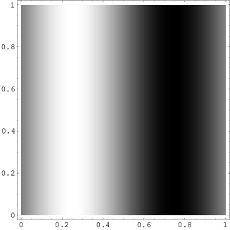
 (yk)2+(yk+)2=N(1ρ2)superscriptsubscriptsuperscript𝑦𝑘2superscriptsubscriptsuperscript𝑦𝑘2𝑁1superscript𝜌2(y^{-}_{k})^{2}+(y^{+}_{k})^{2}=N(1-\rho^{2}), and yν±=0subscriptsuperscript𝑦plus-or-minus𝜈0y^{\pm}_{\nu}=0, for νk𝜈𝑘\nu\neq k, then the states are maximally asymmetric. Namely, they have the cosine shape in the dimension ν=k𝜈𝑘\nu=k, and they are translation invariant across other dimensions, see Fig. 1,

$$x_{j}=\rho+\sqrt{2(1-\rho^{2})}\cos\left[\frac{2\pi(j_{k}-1)}{n}-\alpha_{k}\right].$$

The opposite extreme is the symmetric case $(y^{-}_{\nu})^{2}+(y^{+}_{\nu})^{2}=N(1-\rho^{2})/d$, for $\nu=1,2,\ldots,d$, when the droplet has a rounded-square shape, see Fig. 1,

$$x_{j}=\rho+\sqrt{\frac{2(1-\rho^{2})}{d}}\sum_{\nu=1}^{d}\cos\left[\frac{2\pi(j_{\nu}-1)}{n}-\alpha_{\nu}\right].$$ (16)
Refer to caption
Refer to caption
Figure 1: The shape of the maximally asymmetric and symmetric droplets.

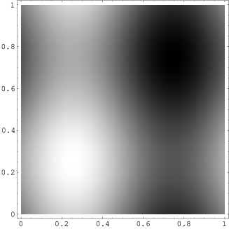
In intermediate situations, the droplet has a kind of elliptic shape, see Fig. 2.

Refer to caption
Figure 2: A droplet of an intermediate shape.

It turns out that the above zero-temperature pure (macro) states are stable with respect to heating up of the system to a temperature not exceeding the critical value $\beta_{c}^{-1}$. Pure (macro) states for $\beta^{-1}>0$ are in one-to-one correspondence with zero-temperature pure states. In the next section we single out pure states for $\beta^{-1}>0$ by quasi-averaging.

6 Quasi-averages.

Pure (micro) states of thermodynamic systems can be obtained with a help of quasi-averaging [1]. The basic recipe of quasi-averaging looks like this: switch on an external field (of magnitude $\varepsilon$) removing the degeneracy of equilibrium state, pass to the thermodynamic limit, switch off the field by sending its magnitude $\varepsilon$ to zero over positive values ($\varepsilon\downarrow 0$). It turns out that in the case of the spherical lattice gas this procedure often deforms macro states (droplet shape). Therefore, we have to use a more potent version of quasi-averaging [2, 3], where the field magnitude is a decreasing function of the volume $N$. That is, the symmetry-breaking external field is switched off together with the thermodynamic limit.

Motivated by the results of the previous section, we begin with the Hamiltonian (2) where the external field

$$h_{j}=\frac{\varepsilon\sqrt{2}}{n^{\delta}}\cos\left[\frac{2\pi(j_{1}-1)}{n}-\alpha\right],\quad j\equiv(j_{1},j_{2},\ldots,j_{d})\in V_{n},$$ (17)

is proportional to an eigenvector corresponding to the second-largest eigenvalue, $\lambda_{\,\rm s}$, of the interaction matrix. The dimensionality of the eigenspace corresponding to $\lambda_{\,\rm s}$ is $2d$, and we are free to choose the value of the parameter $\alpha\in[0,2\pi)$, and instead of $j_{1}$ we can use $j_{\nu}$, with $\nu=2,3,\ldots,d$. Different choices of $\alpha$ and $\nu$ yield different pure macro states.

For the characteristic function of random variables $x_{j}$ and $x_{l}$ one obtains an integral similar to Eq. (11),

$$\chi(t,s)=\frac{\exp(\beta Jd\rho^{2}N)e^{it\rho+is\rho}}{\Theta_{n}(\rho)\sqrt{N}}\frac{\beta J}{2\pi i}\left(\frac{\pi}{\beta J}\right)^{(N-1)/2}\times$$
$$\int_{-i\infty+c}^{+i\infty+c}\!dz\,\exp\left[N\beta\Phi_{n}(z,\varepsilon)\right]\exp\left[-{\sum_{k\in V_{n}}}^{\prime}\frac{\left(tw_{j}^{(k)}+sw_{l}^{(k)}\right)^{2}}{4\beta J(z-\lambda_{k})}\right].$$ (18)

where

$$N\beta\Phi_{n}(z,\varepsilon)=N\beta\Phi_{n}(z)+\frac{i\,\varepsilon}{2Jn^{\delta-d/2}}\frac{tw_{j}^{(2,1,\ldots,1)}+sw_{l}^{(2,1,\ldots,1)}}{z-\lambda_{\rm\,s}}+\underbrace{\frac{\beta\varepsilon^{2}}{4Jn^{2\delta-d}(z-\lambda_{\rm\,s})}}_{\equiv\psi_{n}(z)}.$$

The innocent-looking term $\psi_{n}(z)$ makes a huge difference for the evaluation and behaviour of the integral (18) when $\beta>\beta_{c}$. Indeed, in the scale $z=\lambda_{\rm\,s}+\zeta n^{-\delta}$ the magnitudes of variation of $N\beta\Phi_{n}(z)$ and $\psi_{n}(z)$ with $\zeta$ become comparable. Moreover, if $\delta<d$, then $\psi_{n}(z)$ prevents the saddle point $z_{n}^{*}$ from approaching the pole at $\lambda_{\rm\,s}$ any closer than the distance $O(n^{-\delta})$.

Introducing a new integration variable $\zeta$ via $z=\lambda_{\rm\,s}+\zeta n^{-\delta}$ one obtains

$$N\beta\Phi_{n}(\lambda_{\rm\,s}+\zeta n^{-\delta},\varepsilon)=N\beta\Phi_{n}(\lambda_{\rm\,s}+\zeta n^{-\delta})+$$
$$i\frac{\varepsilon\sqrt{2N}}{2J\zeta}\left\{t\cos\left[\frac{2\pi(j_{1}-1)}{n}-\alpha\right]+s\cos\left[\frac{2\pi(l_{1}-1)}{n}-\alpha\right]\right\}+\frac{n^{d-\delta}\beta\varepsilon^{2}}{4J\zeta}.$$

Gathering the terms of the order $n^{d-\delta}$ and differentiating over $\zeta$ we obtain the following equation for the saddle-point $\zeta^{*}$:

$$(1-\rho^{2})J(\beta-\beta_{c})-\frac{\beta\varepsilon^{2}}{4J\zeta^{2}}=0.$$

Hence the saddle point of $\Phi_{n}(z,\varepsilon)$ is located at

$$z_{n}^{*}=\lambda_{\rm\,s}+\frac{|\varepsilon|}{2Jn^{\delta}}\frac{1}{\sqrt{(1-\rho^{2})(1-\beta_{c}/\beta)}}+o(n^{-\delta}).$$

Application of the saddle-point method to the integral (18) and to the analogous integral for the partition function $\Theta_{n}(\rho)$ shows that the large-$n$ asymptotics of $\chi(t,s)$ coincides with the characteristic function of a bivariate normal distribution ${\cal B}(\mu_{1},\mu_{2};v_{1},v_{2},c)$. That is, for large $n$ the joint distribution of random variables $x_{j}$ and $x_{l}$ is asymptotically normal with mean values $\mu_{1}$ and $\mu_{2}$, variances $v_{1}^{2}$ and $v_{2}^{2}$, respectively, and covariance $c$. Under the assumption that the first components of the nodes $j$ and $l$ scale with $n$ as $j_{1}\sim\gamma n$ and $l_{1}\sim\lambda n$, the expected values of $x_{j}$ and $x_{l}$ are given by

$\displaystyle\mu_{1}=\rho+\sqrt{2(1-\rho^{2})(1-\beta_{c}/\beta)}\cos\left(2\pi\gamma-\alpha\right),$ (19)
$\displaystyle\mu_{2}=\rho+\sqrt{2(1-\rho^{2})(1-\beta_{c}/\beta)}\cos\left(2\pi\lambda-\alpha\right).$ (20)

Note that, provided $\delta\in(0,d)$, the expected values (droplet shape) do not depend on the magnitude of the external field $\varepsilon n^{-\delta}$. Therefore it is reasonable to conclude that the symmetry-breaking field (17) selects one of the possible droplet shapes, but it does not deform the droplet.

The variances $v_{1}^{2}$, $v_{2}^{2}$ and covariance $c(j,l)$ are given by the usual formulae for the pure phases of the spherical model below the critical temperature

$$v_{1}^{2}=v_{2}^{2}=\frac{W_{d}(d)}{2\beta J},$$
$$c(j,l)=\frac{1}{2\beta J}\int_{-\pi}^{\pi}\ldots\int_{-\pi}^{\pi}\frac{\exp\left[i\sum_{\nu=1}^{d}(j_{\nu}-l_{\nu})\omega_{\nu}\right]}{d-\sum_{\nu=1}^{d}\cos\omega_{\nu}}\prod_{\nu=1}^{d}\frac{d\omega_{\nu}}{2\pi}\sim\frac{\Gamma(d/2-1)}{4\beta J\pi^{d/2}r_{j,l}^{d-2}},$$ (21)

where $r_{j,l}$ is the Euclidean distance between $j$ and $l$.

The equations (19) and (20) describe the shape of a localised droplet obtained with a help of the (generalized, see [2, 3]) method of quasi-averages. To double check that the droplet shape (19) is not deformed by the external field we would like to examine the sensitivity of the droplet shape to the type of external field used for quasi-averaging. For this purpose we now repeat the above calculations for a technically more demanding case

$$h_{j}=\left\{\begin{array}[]{cl}\varepsilon n^{-\delta},&\mbox{ if }j_{1}=1,\\ 0,&\mbox{ otherwise,}\end{array}\right.\qquad j\in V_{n};$$ (22)

where $\varepsilon>0$, and $\delta\geq 0$. First, we have to find the range of values for $\delta$, such that the field (22) is strong enough to fix the location of the droplet of condensed “spherical matter”, but, at the same time, it is weak enough not to deform the droplet shape.

The partition function $\Theta_{n}(\rho)$ is still given by Eq. (7), but the coefficients $\varphi_{k}$, $k\in V_{n}$ are now given by

$$\varphi_{k}=\varepsilon n^{d/2-1-\delta}\prod_{\nu=2}^{d}\delta(k_{\nu},1).$$

In order to find the location of the saddle-point of the integrand in Eq. (7) we have to first investigate the behaviour of the sum

$$\Sigma(z)\equiv\frac{1}{4JN}{\sum_{k\in V_{n}}}^{\prime}\frac{\varphi_{k}^{2}}{z-\lambda_{k}}=\frac{\varepsilon^{2}}{4Jn^{2(1+\delta)}}\sum_{k_{1}=2}^{n}\frac{1}{z-d+1-\cos\left[2\pi(k_{1}-1)/n\right]}$$

in the vicinity of the point $z=d$. Fortunately, this sum can be calculated exactly, see [10],

$$\Sigma(z)=\frac{\varepsilon^{2}}{4Jn^{2(1+\delta)}}\left[\frac{2n}{x_{2}(z)-x_{1}(z)}\frac{x_{2}^{n}(z)+1}{x_{2}^{n}(z)-1}-\frac{1}{z-d}\right].$$

Hence, for any fixed $z>d$, the (derivative of the) sum $\Sigma(z)=O(n^{-1-2\delta})$ produces only a vanishing contribution to the saddle-point equation (8).

The contribution of the sum $\Sigma(z)$ becomes significant below the critical temperature, where we have to introduce a new integration variable $\zeta$ via $z=\lambda_{\,\rm s}+\zeta n^{-\gamma}$ before application of the saddle-point method. In order to find the right rescaling for the integration variable $z$ (which, as we shall see shortly, depends on the value of $\delta$ in Eq. (22)), we have to analyse the behavior of $\Sigma(z)$ for different values of $\gamma$.

If $0<\gamma<2$, then

$$\Sigma(\lambda_{\,\rm s}+\zeta n^{-\gamma})\sim\frac{\varepsilon^{2}}{4J\sqrt{2\zeta}}\,n^{-1-2\delta+\gamma/2},\quad\mbox{as $n\to\infty$.}$$

If $\gamma=2$, then

$$\Sigma(\lambda_{\,\rm s}+\zeta n^{-\gamma})\sim\frac{\varepsilon^{2}n^{-2\delta}}{8J}\left(\frac{\coth\sqrt{\zeta/2-\pi^{2}}}{\sqrt{\zeta/2-\pi^{2}}}-\frac{1}{\zeta/2-\pi^{2}}\right),\quad\mbox{as $n\to\infty$.}$$

Note that the r.h.s. of the last equation does not actually have a singularity at $\zeta=2\pi^{2}$. Therefore to find $\Sigma(\lambda_{\,\rm s}+\zeta n^{-\gamma})$ for $\zeta<2\pi^{2}$ one can use the analytic continuation

$$\Sigma(\lambda_{\,\rm s}+\zeta n^{-\gamma})\sim-\frac{\varepsilon^{2}n^{-2\delta}}{8J}\left(\frac{\cot\sqrt{\pi^{2}-\zeta/2}}{\sqrt{\pi^{2}-\zeta/2}}+\frac{1}{\zeta/2-\pi^{2}}\right),\quad\mbox{as $n\to\infty$.}$$

Finally, if $\gamma>2$, then the main asymptotics of $\Sigma(\lambda_{\,\rm s}+\zeta n^{-\gamma})$ comes entirely from the first and the last terms of this sum,

$$\Sigma(\lambda_{\,\rm s}+\zeta n^{-\gamma})\sim\frac{\varepsilon^{2}n^{\gamma-2(1+\delta)}}{2J\zeta},\quad\mbox{as $n\to\infty$.}$$

Under the same rescaling $z=\lambda_{\,\rm s}+\zeta n^{-\gamma}$ the first two terms of $\Phi_{n}(z)$ become

$$J(\lambda_{\,\rm s}+\zeta n^{-\gamma})(1-\rho^{2})-\frac{1}{2\beta N}{\sum_{k\in V_{n}}}^{\prime}\ln(\lambda_{\,\rm s}+\zeta n^{-\gamma}-\lambda_{k})\sim$$
$$J\lambda_{\,\rm s}(1-\rho^{2})-\frac{L_{d}(d)}{2\beta}+n^{-\gamma}\zeta\left[J(1-\rho^{2})-\frac{W_{d}(d)}{2\beta}\right]+n^{-2}\frac{\pi^{2}W_{d}(d)}{\beta}.$$

Hence, if $0<\delta<1$, then the contributions of all $\zeta$-dependent terms in $\Phi_{n}(\lambda_{\,\rm s}+\zeta n^{-\gamma})$ are of the same order when $\gamma=2(1+2\delta)/3$, and the saddle-point equation for $\zeta$ is given by

$$J(1-\rho^{2})(\beta-\beta_{c})=\frac{\beta}{4J}\frac{\varepsilon^{2}}{2\sqrt{2}\zeta^{3/2}}.$$

The positive solution of this equation is given by

$$\zeta^{*}=\frac{1}{2}\left(\frac{\varepsilon}{2J}\right)^{4/3}\frac{1}{\left[(1-\beta_{c}/\beta)(1-\rho^{2})\right]^{2/3}}.$$ (23)

If $\delta=1$, then we have to set $\gamma=2$, which yields the following saddle-point equation for $\zeta$

$$J(1-\rho^{2})(\beta-\beta_{c})=-\frac{\beta\varepsilon^{2}}{8J}\frac{d}{d\zeta}\left(\frac{\coth\sqrt{\zeta/2-\pi^{2}}}{\sqrt{\zeta/2-\pi^{2}}}-\frac{1}{\zeta/2-\pi^{2}}\right).$$ (24)

Finally, if $1<\delta<d-1$, then we have to set $\gamma=1+\delta$, and the saddle-point equation for $\zeta$ is given by

$$J(1-\rho^{2})(\beta-\beta_{c})=\frac{\beta\varepsilon^{2}}{2J\zeta^{2}}.$$

The positive solution of the above equation is given by

$$\zeta^{*}=\frac{\varepsilon}{J\sqrt{2(1-\beta_{c}/\beta)(1-\rho^{2})}}.$$

Now that we know the behavior of the saddle point $z_{n}^{*}$ of the integrand in Eq. (7) we can find the thermodynamic limits of various macro- and microscopic quantities. But before we are able to apply the saddle-point method and find the characteristic function of an arbitrary pair of random variables $x_{j}$ and $x_{l}$ we have to calculate the sum

$$\widetilde{\Sigma}_{j}(z)\equiv{\sum_{k\in V_{n}}}^{\prime}\frac{\gamma_{k}w_{j}^{(k)}}{z-\lambda_{k}},$$

appearing in Eq. (11). After some elementary transformations the above sum reduces to

$$\widetilde{\Sigma}_{j}(z)=\frac{\varepsilon}{n^{1+\delta}}\sum_{k_{1}=2}^{n}\frac{\cos\left[2\pi(j_{1}-1)(k_{1}-1)/n\right]}{z-d+1-\cos\left[2\pi(k_{1}-1)/n\right]},$$

and the summation technique from [10] yields

$$\widetilde{\Sigma}_{j}(z)=\frac{2\varepsilon}{n^{\delta}(x_{2}-x_{1})}\frac{x_{2}^{j_{1}-1}+x_{2}^{n-j_{1}+1}}{x_{2}^{n}-1}-\frac{\varepsilon}{n^{1+\delta}(z-d)}.$$

On application of the saddle-point method to the integral in Eq. (11) one obtains the following expression for the characteristic functions of random variables $x_{j}$ and $x_{l}$:

$$\chi(t,s)\sim\exp\left[-{\sum_{k\in V_{n}}}^{\prime}\frac{\left(tw_{j}^{(k)}+sw_{l}^{(k)}\right)^{2}}{4\beta J\left(z^{*}_{n}-\lambda_{k}\right)}+it\left(\widetilde{\Sigma}_{j}(z^{*}_{n})+\rho\right)+is\left(\widetilde{\Sigma}_{l}(z^{*}_{n})+\rho\right)\right].$$ (25)

Hence, as it is usually the case for pure states of the spherical model, for large values of $n$ the random variables $\{x_{j},j\in V_{n}\}$ have asymptotically normal distributions.

If $\delta\in(0,1)$, then the saddle point is given by $z_{n}^{*}=\lambda_{\,\rm s}+\zeta^{*}n^{-2(1+2\delta)/3}$, see Eq. (23), and the large-$n$ asymptotics of the expected values of the microscopic variables (the multipliers of $it$ and $is$ in Eq. (25)) are given by

xjεn(1δ)/32J2ζ[1+2ζn(1+2δ)/3]j1,similar-todelimited-⟨⟩subscript𝑥𝑗𝜀superscript𝑛1𝛿32𝐽2superscript𝜁superscriptdelimited-[]12superscript𝜁superscript𝑛12𝛿3subscript𝑗1\langle x_{j}\rangle\sim\frac{\varepsilon n^{(1-\delta)/3}}{2J\sqrt{2\zeta^{*}}}\left[1+\sqrt{2\zeta^{*}}n^{-(1+2\delta)/3}\right]^{-j_{1}},

if $j_{1}\leq n/2$. In this case the droplet shape is clearly deformed by the external field, since virtually all “spherical matter” gathers in a narrow layer of the width $\sim n^{(1+2\delta)/3}$ around the hyperplane $j_{1}=1$, where the field is applied.

If $\delta=1$, then the saddle point is given by $z_{n}^{*}=\lambda_{\,\rm s}+\zeta^{*}n^{-2}$, where $\zeta^{*}$ is a solution of Eq. (24), and the large-$n$ asymptotics of the expected values of the microscopic variables are given by

$$\langle x_{j}\rangle\sim\rho+\frac{\varepsilon}{2J}\left[\frac{\cosh\left[(1-2\gamma_{1})\sqrt{\zeta^{*}/2-\pi^{2}}\right]}{\sqrt{2(\zeta^{*}-2\pi^{2})}\sinh\sqrt{\zeta^{*}/2-\pi^{2}}}-\frac{1}{\zeta^{*}-2\pi^{2}}\right].$$ (26)

if $j_{1}\sim\gamma_{1}n$. In this case the droplet shape is still deformed by the external field, since it depends on the field’s magnitude $\varepsilon$.

Finally, if $\delta\in(1,d-1)$, then the large-$n$ asymptotics of the expected values of the thermodynamic variables are given by

$$\langle x_{j}\rangle\sim\rho+\sqrt{2(1-\rho^{2})(1-\beta_{c}/\beta)}\cos\left(2\pi\gamma_{1}\right).$$

if $j_{1}\sim\gamma_{1}n$. In this case, apparently, the droplet shape is not deformed by the external field, since it does not depend on the field’s magnitude $\varepsilon$, and it is the same as in Eqs. (19) and (20).

Thus, the droplet shape is sensitive to the magnitude of the symmetry-breaking field only if it scales with $n$ as $n^{-\delta}$ with $\delta\in[0,1]$. If the field is switched off reasonably fast, $\delta\in(1,d-1)$ in Eq. (22), the droplet shape is not deformed by the field (does not depend on the magnitude of the field). If the field is switched off too fast, $\delta\geq d-1$, then it does not transfer the thermodynamic system into a pure state.

It is appropriate to stress at this point that different configurations of the symmetry breaking field $\{h_{j}:j\in V_{n}\}$ can produce different pure macroscopic phases. Therefore the droplet shape is sensitive to the type of field used for quasi-averaging. The eigenvector (17) is only one of $2d$ orthogonal vectors spanning the eigenspace corresponding to the second-largest eigenvalue of the interaction matrix. In this respect, the symmetry breaking field (22) is special, because it is orthogonal to all of the remaining $2d-1$ eigenvectors corresponding to the eigenvalue $\lambda_{s}$. If instead of the field (22) we decide to use a configuration $\{h_{j}:j\in V_{n}\}$, which has a non-zero scalar product, say, with

$$\sqrt{\frac{2}{n}}\cos\left[\frac{2\pi(j_{2}-1)}{n}-\alpha\right],\quad j\equiv(j_{1},j_{2},\ldots,j_{d})\in V_{n},$$

then the corresponding vector of expected values $\langle x_{j}\rangle$, $j\in{V_{n}}$ will contain a component proportional to $\cos(2\pi j_{2}/n)$, cf. Eq. (16).

7 Discussion.

The investigation of droplet shape performed in this paper demonstrates the importance of decomposing mixed states into constituent pure components. It appears that, often, mixed states are mathematical constructions reflecting absence of sufficient information about the system under investigation. A priori we do not know which of many possible pure states of the system will be actually observed in an experiment. As a consequence, a direct mathematical solution of the model produces a mixed state. At the same time, if an experimentalist actually performs measurement in the corresponding physical system, the obtained results would be described by one of pure states.

Whether this point of view is valid or not, depends, of course, on how quickly the system under investigation can transit from one pure state into another. Namely, if the typical transition time is much larger than the typical experimental observation time, then measurements yield results corresponding to one of pure states. If the observation time is much longer than the transition time, then the observed values are likely to correspond to a mixed state.

Investigation of dynamical properties of the mean spherical model were performed recently, see [5]. It is possible to calculate the interstate transition times using the technique proposed there. We have not attempted yet those calculations, and we do not even know if the droplet shape in the mean spherical and the conventional spherical model are similar. But, it does not seem inconceivable, that the transition time from one pure state into another is much greater than the typical measurement time. Indeed, investigations of large deviation probabilities show that in order to transit from one pure state into another within the conventional spherical model one has to overcome a free-energy barrier that grows exponentially with $n^{d-2}$.

It is well known that gaussian approximations correspond to leading orders of low-temperature expansions of various continuous models. Therefore, one can hope that the behaviour of realistic continuous models, for instance $O(n)$ models, is qualitatively similar to the findings of the present paper. On the other hand, the common knowledge is that physical substances in liquid phases form droplets which boundaries are sharp in the macroscopic scale. Most likely, the sharpness of boundaries should be attributed to the atomistic (discrete) microscopic structure of physical substances. Therefore, in this respect, discrete lattice gas models of Ising type provide much more realistic description of various substances in the liquid state.

References

  • [1] N. N. Bogolubov, On some problems of the theory of superconductivity, Physica, Suppl. to vol. 26:S1–S16 (1960).
  • [2] N. Angelescu and V. A. Zagrebnov, A generalized quasiaverage approach to the description of the limit states of the $n$-vector Curie-Weiss ferromagnet, J. Stat. Phys. 41:323–334 (1985).
  • [3] J. G. Brankov, V. A. Zagrebnov, and N. S. Tonchev, Description of the limit Gibbs states for the Curie-Weiss-Ising model, Theor. Math. Phys. 66:72–80 (1986).
  • [4] R. L. Dobrushin, R. Kotecký, and S. Shlosman, Wulff Construction: A Global Shape from Local Interaction, (AMS translation series, Providence, 1992).
  • [5] C. Godrèche and J. M. Luck, Response of Non-Equilibrium Systems at Criticality: Ferromagnetic Models in Dimension Two and Above, J. Phys. A: Math. Gen. 33:9141–9164 (2000).
  • [6] H. A. Gersch and T. H. Berlin, Spherical Lattice Gas, Phys. Rev. 127:2276–2283 (1962).
  • [7] J. Glimm and A. Jaffe, Quantum Physics: A Functional Integral Point of View. (Springer-Verlag, Berlin, 1981).
  • [8] R. A. Minlos and Y. G. Sinai, The phenomenon of ”phase separation” at low temperatures in some lattice models of a gas. I, Matem. Sbornik. 73:375–448 (1967).
  • [9] R. A. Minlos and Y. G. Sinai, The phenomenon of ”phase separation” at low temperatures in some lattice models of a gas. II, Trans. Moscow Math. Soc. 19:113–178 (1968).
  • [10] A. E. Patrick, The influence of external boundary conditions on the spherical model of a ferromagnet. I. Magnetization profiles, J. Stat. Phys. 75:253–295 (1994).
  • [11] W. Pressman and J. B. Keller, Equation of State and Phase Transition of the Spherical Lattice Gas, Phys. Rev. 120:22–32 (1960).
  • [12] Ya. G. Sinai, Mathematical Problems in Statistical Mechanics, (World-Scientific, Singapore, 1991).