Dilaton stabilization by massive fermion matter

Abstract

The study started in Ref. jcap about the Dilaton mean field stabilization thanks to the effective potential generated by the existence of massive fermions, is here extended. Three loop corrections are evaluated in addition to the previously calculated two loop terms. The results indicate that the Dilaton vacuum field tend to be fixed at a high value close to the Planck scale, in accordance with the need for predicting Einstein gravity from string theory. The mass of the Dilaton is evaluated to be also a high value close to the Planck mass, which implies the absence of Dilaton scalar signals in modern cosmological observations. These properties arise when the fermion mass is chosen to be either at a lower bound corresponding to the top quark mass, or alternatively, at a very much higher value assumed to be in the grand unification energy range. One of the three 3-loop terms is exactly evaluated in terms of Master integrals. The other two graphs are however evaluated in their leading logarithm correction in the perturbative expansion. The calculation of the non leading logarithmic contribution and the inclusion of higher loops terms could made more precise the numerical estimates of the vacuum field value and masses, but seemingly are expected not to change the qualitative behavior obtained. The validity of the here employed Yukawa model approximation is argued for small value of the fermion masses with respect to the Planck one. A correction to the two loop calculation done in the previous work is here underlined.

Accepted for publication in Astrophysics and Space Science.

I Introduction

The Dilaton is an essential ingredient of superstring theory, and constitutes a scalar field partner of the graviton GSW .  Therefore, the background fields associated with the vacuum state of superstring theory should involve this field in common with the metric in the basic action. This is referred to as Dilaton gravity Ven ; TV . To the lowest level of approximation the Dilaton is a free and massless scalar field with a special kind of coupling to the matter fields. As a consequence of this coupling, a time varying Dilaton field determines time-dependent coupling constants. In order to overcome this difficulty the Dilaton should remain constant during the present stage of evolution of the Universe. Moreover, unless the Dilaton turns out to be very massive, its existence could lead to an observable “Fifth force” similar to the ones which are currently associated to the observations of the Dark Matter. The constraints posed by current experimental observations determine the lower bound on the mass of the Dilaton to be of the order $m<10^{-12}\mathrm{GeV}$ bound (but see Polyakov for an attempt to make a running Dilaton consistent with late time cosmology).

The Dilaton stabilization problem has been at the center of an intense research activity in recent times because of its physical relevance. It should be emphasized that the Dilaton is one of various scalar fields appearing in the formulation of superstring theory in the low-energy limit. The sizes and shapes of the extra spatial dimensions associated with superstring theory are also leading to additional scalar fields, called “moduli fields”. The stabilization of such moduli fields has been the object of recent attention particularly in connection with Type IIB superstring theory. The introduction of fluxes within the compactification spaces has made it possible to stabilize various moduli fields GKP . Also, gaugino condensation gaugino has been employed to stabilize the Dilaton field in the context of heterotic superstring theory heterotic and in string gas cosmology Danos .

It should be remarked that, since Dilaton stabilization has special relevance for late time cosmology, there is motivation for finding mechanisms which do not directly rest on the concrete assumptions defining the nature of the extra dimensions. An additional motivation to search for alternative Dilaton stabilization mechanisms comes from String Gas Cosmology (SGC). The SGC BV ; SGCrevs is a model of early universe cosmology which employs new degrees of freedom and symmetries of string theory, and couples these elements with gravity and Dilaton fields into a classical action background model. The Universe is considered to start as a compact space containing a gas of strings. Since in string theory there is a maximal temperature for a gas of closed strings, the initial state of the cosmological evolution in SGC will be a phase of almost constant temperature, the so called ”Hagedorn phase”. The SGC is able to define a non-singular cosmology in which there is no starting Big Bang explosion. It has been noted that the thermal fluctuations in a gas of closed strings in the Hagedorn phase can justify the scale-invariant spectrum of cosmological fluctuations observed in Nature NBV ; BNPV2 , with a particular prediction of a slight blue tilt for gravitational waves BNPV1 . However, the consistency of the picture requires that the Dilaton field be fixed during the Hagedorn phase. Therefore, in the SGC theory the Dilaton needs to be fixed at very early times and at very late times.

Thus, clarifying the mechanisms of Dilaton field stabilization is an important question in particle physics today. It is worth noting that the universal type of coupling of the Dilaton to the matter fields not only leads to an unwanted effect as the time-dependence of the coupling constants but it also furnishes the possibility that quantum effects due to the interaction of the Dilaton with matter might generate interesting contributions to the effective potential of the Dilaton.

In a previous work published in Ref. jcap , we started to explore this question. The work considered the cosmological periods when the additional spatial dimensions of superstring theory were already stabilized and the study was done in the framework of a four-dimensional field theory. The objective of study was then the interaction of the Dilaton with massive fermions. Such masses can be defined by fluxes about internal manifolds. In late time cosmology, the masses could had been generated after supersymmetry breaking. In an alternative early universe cosmology, one may consider thermally generated fermion masses. In Ref. jcap it was considered a simple form for the Dilaton gravity action in which a massive Dirac fermion term was added elizalde . The action was chosen in the Einstein frame, which does not show any Dilaton field dependence in the kinetic terms for the fermions. On the other hand, the fermion mass becomes a function of the Dilaton, involving a universal exponential factor in Dilaton gravity Ven ; TV . The chosen action described the low energy effective interaction of Super-Yang-Mills fermions with the Dilaton field in superstring theory jcap . The effective potential for the Dilaton field was evaluated up to two loop corrections in the small Dilaton radiative quantum field limit.  That leads to a Yukawa like interaction term which allows standard QFT calculations. A fixed value of the cosmological scale factor was assumed. The outcome of the work was, thanks to the appearing of logarithms in the loop calculations, that the Dilaton field appeared in the result in powers multiplied by the exponential factors of the field. This structure, in the one loop approximation clearly indicated the spontaneous generation of vacuum mean value of the Dilaton field.

Motivated by the dynamical generation of the Dilaton result in Ref. jcap , we here will address the evaluation of next corrections 3-loop terms to the 2-loop evaluation of the effective potential for the Dilaton field. The main issue to be  explored is the possibility of the appearance in the improved potential  of the stabilizing effect which were in fact absent in the second order correction, and which are suspected to be created by the existence of massive matter upon the mean value of the Dilaton.

The results obtained, at least indicate, for the fermion mass being selected at the $GUT$ or the $top$ quark mass scales, that the mean value of the Dilaton field tends to be stabilized at a high value being close to the Planck mass or the $GUT$ scale, respectively. Therefore, it is suggested that the appearance of mass for matter in the course of the evolution of the Universe can generate a stabilizing action on the vacuum expectation value of the Dilaton field making it unobservable. This effect will tend to stop the time evolution of the mean value, as it is convenient for String Theory consistency.

The work also present an study of the validity of the linear approximation of the Dilaton exponential factor which leads to the simpler effective Yukawa theory employed. It follows that for the two values of the large fermion masses assumed (the top quark and GUT scale ones) the approximation should work well, after assuming that the low energy effective effective action of string theory is the bare one in the renormalization of the model. A brief resume about the procedure employed to estimate the Dilaton mass is also given.

We can point out, that in the process extending the work to include higher loop corrections, we have noticed that in Ref. jcap the kinetic term of the Dilaton Lagrangian was chosen with a negative sign. This selection, although not changing the one loop correction, led to a sign change of the 2-loop terms, which suggested the existence of minima in the effective action argued in Ref. jcap . However, in spite of this non physical adopted assumption in that work, the indication about the dynamical generation in Ref.jcap remained a valid one, because the change in the metric did not affected the one-loop correction, the basic quantity indicating the dynamical generation effect. The present work corrects the result for the two loop terms, and indicates that its place in the stabilizing effect over the Dilaton field is played by higher order contributions.

The paper proceeds as follows: In Section II, the notation and basic formulation are given. Section III presents the elements of the three loops evaluation of the effective potential.  Section IV  discuss the results of the calculation.  In Section V the results are resumed and commented. Finally, Appendix A presents the investigation of the Yukawa model approximation and the review on the scheme for evaluating the generated Dilaton mass.

II The Dilaton action and generating functional

Let us consider a model of the Dilaton field interacting with fermion matter in the form

$$S\, = \,\int d^{4}x\sqrt{-g(x)}{\LARGE(}\frac{1}{2\kappa^{2}}g^{\mu\nu}(x)\partial_{\mu}\phi^{r}(x)\partial_{\nu}\phi^{r}(x)+\overline{\Psi}(x)(i\frac{g^{\mu\nu}\gamma_{\mu}\overleftrightarrow{\partial}_{\nu}}{2}-m)\Psi(x)$$ (1)

$$\,-\overline{\Psi}(x)g_{Y\text{ }}^{*}\phi^{r}(x)\Psi(x)+j(x)\phi^{r}(x)+\overline{\Psi}(x)\eta(x)\text{ \ +}\overline{\eta}(x)\Psi(x){\LARGE)},$$

$$m = \exp(\alpha^{*}\text{ }\phi)m_{f},$$ (2)

$$g_{Y}^{*} = \alpha^{*}\text{ }m,$$ (3)

$$\alpha^{*} = -\frac{3}{4},$$ (4)

$$\text{ \ \ \ \ }x^{\mu} = (x^{0},x^{1},x^{2},x^{3}),\text{ \ \ \ }\overleftrightarrow{\partial}=\overrightarrow{\partial}-\overleftarrow{\partial},\text{ \ }\left\{\gamma_{\mu},\gamma_{\nu}\right\}=2g_{\mu\nu}(x),$$ (5)

$$g_{\mu\nu}(x) = \left(\begin{array}[]{llll}1&0&0&0\\ 0&-1&0&0\\ 0&0&-1&0\\ 0&0&0&-1\end{array}\right),\text{ \ \ }\sqrt{-g(x)}=1.$$ (10)

That is, we are considering  the Dilaton field  interacting with a massive fermion in the Einstein frame, in which the metric $g_{\mu\nu}$ has been approximated by the Minkowski metric in order to simplify the evaluation. The gravitational constant is here explicitly introduced, and natural units are employed for the distances and mass. The vacuum value of the Dilaton field is named as $\phi$ and its radiative part is called $\phi^{r}.$ Note that we are assuming the radiative part is small in order to retain only the first term in the  expansion of the exponential. This is the Yukawa approximation which is here employed. In appendix A it is argued that it can be a a good approximation for the two values of the large fermion masses considered here : the top quark mass and a GUT scale one, assumed that the the ratio between the fermion mass and the Planck one is very much smaller than one. All the results will be functions of the vacuum field $\phi$ and the fermion mass $m$.

The parameter defining the Dilaton field dependent exponential, the Planck length $\kappa=$ $l_{P}$ and mass $m_{P}$ are defined by the expressions

$$\kappa^{2} = \frac{8\pi G\hbox to0.0pt{\rule[4.73611pt]{3.24997pt}{0.43057pt}\hss}h}{c^{3}},$$ (11)

$$\kappa = l_{P}=\frac{1}{m_{P}}=8.10009\times 10^{-33}\ \text{cm},$$ (12)

$$G = 6.67\times 10^{-8}\ \text{cm}^{3}\ \text{g}^{-1}\ \text{s}^{-2},$$ (13)

$$\hbar = 1.05457\times 10^{-27}\ \text{cm}^{2}\ \text{g}\ \text{s}^{-1},$$ (14)

$$c = 2.9979245800\times 10^{10}\ \text{cm}\ \text{s}^{-1}.$$ (15)

In the above formula for the action, the coordinates and times are measured in cm, the masses $m$ in the natural unit cm^-1 and the Dilaton field is dimensionless.

Starting from the classical action, we will consider a 3-loop correction to the effective action, assuming a homogenous and time independent value of the Dilaton mean field $\phi$ as

$$\frac{\Gamma[\phi]}{V^{(4)}}=-V^{eff}(\phi),$$ (16)

where $V^{(4)}$ is the four dimensional volume. In order to eliminate the explicit appearance of the gravitational constant from the diagram technique for evaluating the effective action, we could absorb it by redefining the Dilaton field value and the $\alpha^{*}$ constant as

$$\ \varphi = \phi/\kappa,$$ (17)

$$\alpha = \alpha^{*}\kappa=-\frac{3}{4}\kappa,$$ (18)

$$g_{Y} = g_{Y}^{*}\kappa.$$ (19)

After these changes, the above written classical action $S,$ to be used for generating the Feynman expansion can be expressed as follows

$$S\,[\overline{\Psi},\Psi,\varphi^{r},\varphi] = \,\int d^{4}x\text{ }{\Large(}\frac{1}{2}g^{\mu\nu}(x)\partial_{\mu}\varphi^{r}(x)\partial_{\nu}\varphi^{r}(x)+\overline{\Psi}(x)(i\frac{g^{\mu\nu}\gamma_{\mu}\overleftrightarrow{\partial}_{\nu}}{2}-m)\Psi(x)$$ (20)

$$-\overline{\Psi}(x)g_{Y\text{ }}\varphi^{r}(x)\Psi(x)+j(x)(\text{ }\varphi+\varphi^{r}(x))+\overline{\Psi}(x)\text{ }\eta(x)\text{ \ +}\overline{\eta}(x)\text{ }\Psi(x){\Large)}.$$

The expansion is considered in $\ d=4-2\epsilon$ dimensions for implementing dimensional regularization scheme. Accordingly, the coupling constant $g_{Y\text{ }}$ should be modified  by the introduction of the regularization scale parameter $\mu$ as  follows

$$g_{Y\text{ }}^{2}=\mu^{2\epsilon}(g_{Y\text{ }}^{0})^{2},$$

where $g_{Y\text{ }}^{0}$ is the usual coupling constant in four dimensions.

II.1 The generating functional and  the effective action

In this subsection, for the sake of definiteness, we will sketch the main expressions defining the perturbative calculation to be considered  in what follows.   The generating functional of the Green functions $Z$ , its connected part $W$  and the mean field values will defined by the formulae

$$Z[\overline{\eta},\eta,j] = \int\mathcal{D}\overline{\Psi}\mathcal{D}\Psi\mathcal{D}\varphi^{r}\exp(i\text{ }S\,[\overline{\Psi},\Psi,\varphi^{r},\varphi]),$$ (21)

$$W[\overline{\eta},\eta,j] = \frac{1}{i}\log Z[\overline{\eta},\eta,j],$$ (22)

$$\frac{\delta\text{ }W}{i\text{ }\delta j(x)} = \varphi+\langle\varphi^{r}(x)\rangle,$$ (23)

$$\frac{\delta\text{ }W}{i\text{ }\delta\overline{\eta}(x)} = \langle\Psi(x)\rangle,$$ (24)

$$\frac{\delta\text{ }W}{-i\text{ }\delta\eta(x)} = \langle\overline{\Psi}(x)\rangle.$$ (25)

Note that the mean Dilaton field $\varphi$ is considered as homogeneous and the mean value of the radiative part $\langle\varphi^{r}(x)\rangle$ will be assumed to vanish when the sources are zero.  The effective action is defined as the Legendre transform of $Z$  depending on the mean field values as:

$$\Gamma[\langle\Psi\rangle,\langle\overline{\Psi}\rangle,\varphi+\langle\varphi^{r}\rangle] = \frac{1}{i}\log Z[\overline{\eta},\eta,j]-\int dx{\Large[}j(x)(\text{ }\varphi+\langle\varphi^{r}(x)\rangle)+\langle\overline{\Psi}(x)\rangle\text{ }\eta(x)\text{ \ +}\overline{\eta}(x)\text{ }\langle\Psi(x)\rangle{\Large\ ]},$$ (26)

$$\frac{\delta\text{ }\Gamma}{\delta\langle\varphi^{r}(x)\rangle} = -j(x),$$ (27)

$$\frac{\delta\text{ }\Gamma}{\delta\langle\overline{\Psi}(x)\rangle} = -\eta(x),$$ (28)

$$\frac{\delta\text{ }\Gamma}{\delta\langle\Psi(x)\rangle} = \overline{\eta}(x).$$ (29)

The expression for $Z,$ after writing the Yukawa vertex part of the Lagrangian in terms of the functional derivatives over the sources and integrating the gaussian functional integral that remains, leads to the Wick expansion  formula:

$$Z[\overline{\eta},\eta,j] = \exp{\large[}i\int dx\text{ }g_{Y}\frac{\delta}{i\delta j(x)}\frac{\delta}{-i\delta\eta(x)}\frac{\delta}{i\delta\overline{\eta}(x)}{\large]\times}$$ (30)

$$\exp\left[\int dx\text{ }dy\text{ }{\LARGE(}\overline{\eta}(x)S(x-y)\eta(y)+\frac{1}{2}j(x)D(x-y)j(y){\LARGE)}\right],$$

$$S(x-y) = \int\frac{dp^{d}}{(2\pi)^{d}}\frac{\exp(-i\text{ }p.(x-y))}{m-\gamma^{\mu}p_{\mu}},$$ (31)

$$D(x-y) = \int\frac{dk^{d}}{(2\pi)^{d}}\frac{\exp(-i\text{ }k.(x-y))}{-(k^{2}-i\epsilon)},$$ (32)

in which $\ S$ and $D$ are the fermion and Dilaton free propagators, respectively.  The notation for fermions and scalar field related quantities, and the definition of the Feynman rules for the   generation of the analytic expressions for the various contributions are exactly the ones described in Ref. muta , for the cases of scalar and fermion fields.   Specifically, for the momentum space rules, the propagators and  the only existing vertex are graphically illustrated in figure 1.

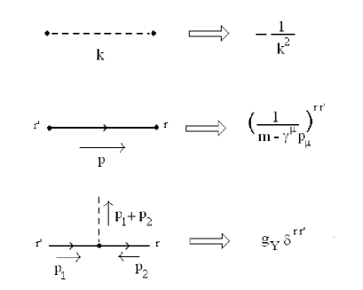
Figure 1: The figure illustrates the Feynman rules for the particular Yukawa model approximation adopted for the Dilaton action

III Effective potential evaluation

Let us present in this section the evaluations of the effective potential for the Dilaton field following after employing the perturbative expansion described in the past section.  The diagrams to be considered are depicted in Fig. 2. They include up two three loop corrections.  The contributions will be exactly evaluated for the one and two loops.  In addition, the three loop term $D_{32}$ also can be analytically calculated in terms of Master integrals.  However, the three loop diagrams $D_{31}$ and $D_{33}$  are here determined only in their leading terms of order $\log\left(\frac{m}{\mu}\right)^{3}$ . We expect to be able in evaluating the non leading corrections (lower powers of $\ log\left(\frac{m}{\mu}\right)$) in extending the work. Let us discuss the results for each diagram in various subsections below.

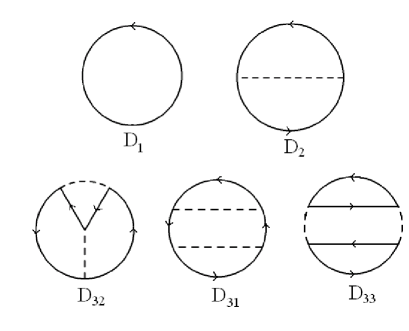
Figure 2: The one, two and three loops Feynman diagrams considered in this work. The one and two loop corrections $D_{1}$ and $D_{2}$ are exactly calculated. In the case of the three loops terms, the $D_{32}$ is completely evaluated in terms of the listed Master integrals in Ref. schavuor . The $D_{31}$ and $D_{33}$ were determined only in their leading logarithm correction.

III.1 One loop term $D_{1}$

The analytic expression for the one loop diagram $\ D_{1}$ and its derivative over $m^{2}$ have the forms

$$\Gamma^{(1)} = V^{(d)}\int\frac{dp^{d}}{(2\pi)^{d}i}Tr\log(m^{2}-p^{2}),$$ (33)

$$\frac{d}{d\text{ }m^{2}}\Gamma^{(1)} = 4V^{(d)}\int\frac{dp^{d}}{(2\pi)^{d}i}\frac{1}{m^{2}-p^{2}}.$$ (34)

The result for the momentum integral entering in the derivative of $\ \Gamma^{(1)}$ over $m^{2},$ after divided by $\mu^{2\epsilon}$ $V^{(d)}$ (in order to define a 4-dimensional energy density)  and integrated over $m^{2}$, allows to write for the one loop effective action density (See Ref. schavuor )

$$\gamma_{1}(m,\epsilon,\mu)\equiv\frac{\Gamma^{(1)}}{\mu^{2\epsilon}V^{(d)}}=m^{4}(\frac{m}{\mu})^{-2\epsilon}\frac{8\pi^{2-\epsilon}}{(2\pi)^{4-2\epsilon}}\Gamma(-1+\epsilon).$$ (35)

After employing the minimal substraction (MS) scheme, that is, getting the finite part by eliminating the pure pole part in $\epsilon$ the Laurent expansion  of $\gamma(m,\epsilon)$ and taking the limit $\epsilon\rightarrow 0,$  the one loop contribution to the effective action density as a function of $\ m$ and $\mu$   becomes

$$\gamma_{1}(m,\mu)=0.0506606m^{4}\left(2.\log\left(\frac{m}{\mu}\right)-2.95381\right).$$ (36)

Note that the negative of this term, which gives the one loop effective potential  leads to a the dynamical generation of the Dilaton field for positive values of $\alpha^{*}$ $\phi$ as follows from $log(m)=log(m_{f})$ $+\alpha^{*}$ $\phi.$ This was the effect which motivated the study started in  Ref. jcap .

III.2 Two loop term $D_{2}$

For the  two loop contribution  $D_{2}$  the analytic expression is

$$\gamma_{2}(m,\epsilon,\mu) \equiv \frac{\Gamma^{(2)}}{\mu^{2\epsilon}V^{(d)}}=\frac{1}{2}(g_{Y\text{ }}^{0})^{2}\text{ }\int\frac{dp_{1}^{d}}{(2\pi)^{d}i}\frac{dp_{2}^{d}}{(2\pi)^{d}i}\frac{4(m^{2}+p_{1}.p_{2})}{(m^{2}-p_{1}^{2})(m^{2}-p_{2}^{2})(p_{1}-p_{2})^{2}}$$ (37)

$$= \frac{1}{2}(g_{Y\text{ }}^{0})^{2}m^{2d-4}\int\frac{dq_{1}^{d}}{(2\pi)^{d}i}\frac{dq_{2}^{d}}{(2\pi)^{d}i}\frac{4(1+q_{1}.q_{2})}{(1-q_{1}^{2})(1-q_{2}^{2})(q_{1}-q_{2})^{2}}$$

$$= 2(g_{Y\text{ }}^{0})^{2}m^{4}m^{-4\epsilon}{\Huge(}2\int\frac{dq_{1}^{d}}{(2\pi)^{d}i}\frac{dq_{2}^{d}}{(2\pi)^{d}i}\frac{1}{(1-q_{1}^{2})(1-q_{2}^{2})(q_{1}-q_{2})^{2}}-$$

$$-\frac{1}{2}(\int\frac{dq_{1}^{d}}{(2\pi)^{d}i}\frac{1}{(1-q_{1}^{2})})^{2}{\Huge)},$$

where the identity $q_{1}.q_{2}=\frac{1}{2}(q_{1}^{2}-1+q_{{}_{2}}{}^{2}-1)+1-\frac{1}{2}(q_{1}-q_{2})^{2}$ has been used.  The two momentum integrals appearing in the last line are the simplest Master integrals for scalar fields as listed in Ref. schavuor . The results for them in that reference are:

$$\int\frac{dq_{1}^{d}}{(2\pi)^{d}i}\frac{dq_{2}^{d}}{(2\pi)^{d}i}\frac{1}{(1-q_{1}^{2})(1-q_{2}^{2})(q_{1}-q_{2})^{2}} = \frac{(d-2)(\pi)^{d}\Gamma\left(1-\frac{d}{2}\right)^{2}}{2(d-3)(2\pi)^{2d}},$$ (38)

$$\int\frac{dq_{1}^{d}}{(2\pi)^{d}i}\frac{1}{(1-q_{1}^{2})} = \frac{(\pi)^{\frac{d}{2}}\Gamma\left(1-\frac{d}{2}\right)}{(2\pi)^{d}}.$$ (39)

They allow to write for the regularized two loop effective action density the expression

$$\gamma_{2}(m,\epsilon,\mu)=-m^{4}(\frac{m}{\mu})^{-4\epsilon}\frac{2(g_{Y\text{ }}^{0})^{2}(\pi)^{d}}{(2\pi)^{2d}}(-\frac{d-2}{d-3}+\frac{1}{2})\Gamma\left(1-\frac{d}{2}\right)^{2}.$$ (40)

Expanding in Laurent series in $\epsilon$ and disregarding the  pole part  in the limit $\epsilon\rightarrow 0$, leads to the two loop perturbative contribution to the effective action

$$\gamma_{2}(m,\mu)=\text{ \ }0.0000200507\text{(}g_{Y\text{ }}^{0})^{2}m^{4}\text{ }{\Huge(}48.\log^{2}\left(\frac{m}{\mu}\right)-173.783\log\frac{m}{\mu}\text{ \ }+183.83\ {\Huge)}.$$ (41)

As it was noticed in the Introduction, in Ref. jcap it was employed an inappropriate negative kinetic term for the Dilaton field. This change, although not affecting the one fermion loop contribution, which is not altered by the sign of the boson propagator,  drastically modified the sign of the two loop term which linearly depends on the Dilaton propagator.  In the  previous evaluation, the two loop terms determined the existence of minima for the Dilaton potential. Therefore, the consequence of the change in sign fixed by the here consideration of the correct positive kinetic energy term, should be investigated in connection with the existence of stabilizing minima for the scalar field. This circumstance determined the motivation for the new three loop corrections considered in this work.

III.3 Three loops terms

Let us now consider the three loop terms.

III.3.1 Diagram  $D_{32}$

The $D_{32}$ term is the only of the 3-loops diagrams which is not composed of two fermion or boson self energy insertions connected in series. For the $D_{31}$ and $D_{33}$ cases we had difficulties in reducing their contributions to a linear combination of  tabulated Master integrals. This obstacle only allowed us to calculate their leading term in the expansion in $\log(\frac{m}{\mu}).$  However, for $D_{32}$ it was possible to express it as a sum over the Master integrals  given in Ref. schavuor . The analytic expression of the diagram is

$$\Gamma^{(32)} = -V^{(d)}\frac{1}{4}(g_{Y})^{4}\int\frac{dp_{1}^{d}}{(2\pi)^{d}i}\frac{dp_{2}^{d}}{(2\pi)^{d}i}\frac{dp_{3}^{d}}{(2\pi)^{d}i}\times$$ (42)

$$\frac{\text{Tr}\left[(m+p_{2}^{\mu}\gamma_{\mu})(m+(p_{2}^{\mu}+p_{3}^{\mu}-p_{1}^{\mu})\gamma_{\mu})(m+p_{3}^{\mu}\gamma_{\mu})(m+p_{1}^{\mu}\gamma_{\mu})\right]}{(m^{2}-p_{1}^{2})(m^{2}-p_{2}^{2})(m^{2}-p_{3}^{2})(m^{2}-(p_{2}+p_{3}-p_{1})^{2})(p_{1}-p_{3})^{2}(p_{1}-p_{2})^{2}}$$

$$= -V^{(d)}\frac{1}{4}(g_{Y})^{4}\int\frac{dp_{1}^{d}}{(2\pi)^{d}i}\frac{dp_{2}^{d}}{(2\pi)^{d}i}\frac{dp_{3}^{d}}{(2\pi)^{d}i}\times$$

$$\frac{m^{4}+c_{1}(p_{1},p_{2},p_{3})m^{2}+c_{2}(p_{1},p_{2},p_{3})}{(m^{2}-p_{1}^{2})(m^{2}-p_{2}^{2})(m^{2}-p_{3}^{2})(m^{2}-(p_{2}+p_{3}-p_{1})^{2})(p_{1}-p_{3})^{2}(p_{1}-p_{2})^{2}},$$

$$c_{1}(p_{1},p_{2},p_{3}) = 3p_{2}.p_{3+}p_{1}.p_{2}+p_{1}.p_{3}+p_{2}^{2}+p_{3}^{2}-p_{1}^{2}\text{ \ \ \ \ }$$ (43)

$$c_{2}(p_{1},p_{2},p_{3}) = p_{1}^{2}\text{ }p_{2}.p_{3}+p_{2}^{2}\text{ }p_{1}.p_{3}+p_{3}^{2}\text{ }p_{1}.p_{2}-2\text{ }p_{1}.p_{2}\text{ }p_{1}.p_{3}.$$ (44)

Defining now

$$z_{1} = p_{1}^{2}-m^{2},$$

$$z_{2} = p_{2}^{2}-m^{2},$$

$$z_{3} = p_{3}^{2}-m^{2},$$

$$z_{4} = (p_{1}-p_{2})^{2},$$

$$z_{5} = (p_{1}-p_{3})^{2},$$

$$z_{6} = (p_{2}-p_{1}+p_{3})^{2}-m^{2},$$ (45)

and employing various vectorial identities expressing the squares of the differences between any two momenta in terms of the scalar product between them and the squares of the considered momenta, the integral defining $\Gamma^{(32)}$ can be written as follows

$$\Gamma^{(32)} = -V^{(d)}\frac{1}{4}(g_{Y\text{ }})^{4}\int\frac{dp_{1}^{d}}{(2\pi)^{d}i}\frac{dp_{2}^{d}}{(2\pi)^{d}i}\frac{dp_{3}^{d}}{(2\pi)^{d}i}\times$$

$$\frac{m^{4}+c_{1}(z)\text{ }m^{2}+c_{2}(z)}{z_{1}\text{ }z_{2}\text{ }z_{3}\text{ }z_{4}\text{ }z_{5}\text{ }z_{6}},$$

$$z = (z_{1}\text{, }z_{2},z_{3},\text{ }z_{4},\text{ }z_{5}\text{,}z_{6}),$$ (46)

$$c_{1}(z) = \frac{3}{2}(z_{1}+\text{ }z_{2}+\text{ }z_{3}+z_{6})-2(\text{ }z_{4}\text{ }+z_{5})\text{ }+6m^{2},$$ (47)

$$c_{2}(z) = \frac{1}{2}(z_{1}z_{6}+z_{2}z_{3}-z_{4}z_{5}+m^{2}(z_{1}+z_{2}+z_{3}+z_{6})+2m^{4}).$$ (48)

Therefore, there are one or two $z$ factors in the denominator that can be canceled by the terms of the quadratic polynomial in these quantities. This allows the integral to be decomposed in a linear combination of the Master integrals listed in Ref. schavuor . The result for    action density

$$\gamma_{32}(m,\mu,\epsilon)=\frac{\Gamma^{(32)}}{\mu^{2\epsilon}V^{(d)}},$$

can be expressed in terms of only five of them as follows

$$\gamma_{32}(m,\mu,\epsilon)=-(g_{Y\text{ }}^{0})^{4}\text{ }m^{4}\left(\frac{m}{\mu}\right)^{-6\epsilon}\left(8I_{1}(\epsilon)+8I_{2}(\epsilon)-4I_{3}(\epsilon)+I_{5}(\epsilon)-\frac{I_{7}(\epsilon)}{2}\right),$$

where the functions $I_{1}(\epsilon)$, $I_{2}(\epsilon),I_{3}(\epsilon),I_{5}(\epsilon)$ and $I_{7}(\epsilon)$ result to be given by

$$I_{1}(\epsilon) = \frac{2^{-3(4-2\epsilon)-9}\pi^{-\frac{3}{2}(4-2\epsilon)}(5(4-2\epsilon)-18)M_{1}(\epsilon)^{3}}{1-2\epsilon}+$$ (49)

$$\frac{2^{-3(4-2\epsilon)-6}\pi^{-3(4-2\epsilon)}(3(4-2\epsilon)-10)(3(4-2\epsilon)-8)\left(M_{5}(\epsilon)-\frac{8\epsilon}{2(4-2\epsilon)-7}M_{4}(\epsilon)\right)}{\epsilon^{2}},$$

$$I_{2}(\epsilon) = -\frac{2^{-3(4-2\epsilon)-2}\pi^{-3(4-2\epsilon)}}{1-2\epsilon}\left(\frac{M_{1}(\epsilon)^{3}(2-2\epsilon)^{2}}{1-2\epsilon}+(3(4-2\epsilon)-8)M_{4}(\epsilon)\right),$$ (50)

$$I_{3}(\epsilon) = -\frac{2^{-3(4-2\epsilon)-3}\pi^{-3(4-2\epsilon)}}{\epsilon}\left(\frac{2(2-2\epsilon)^{2}M_{1}(\epsilon)^{3}}{1-2\epsilon}+(3(4-2\epsilon)-8)M_{5}(\epsilon)\right),$$ (51)

$$I_{5}(\epsilon) = (2\pi)^{-3(4-2\epsilon)}M_{4}(\epsilon),$$ (52)

$$I_{7}(\epsilon) = (2\pi)^{-3(4-2\epsilon)}M_{5}(\epsilon),$$ (53)

in terms of the Master integrals (See Ref. schavuor ):

$$M_{1}(\epsilon) = \pi^{\frac{1}{2}(4-2\epsilon)}\Gamma\left(\frac{1}{2}(2\epsilon-4)+1\right),$$ (54)

$$M_{2}(\epsilon) = -\frac{(2-2\epsilon)\text{ }M_{1}(\epsilon)^{2}}{2(1-2\epsilon)},$$ (55)

$$M_{3}(\epsilon) = 2^{\frac{1}{2}(2\epsilon-4)}\Gamma\left(\frac{1}{2}(4-2\epsilon)\right)\Gamma\left(\frac{1}{2}(2\epsilon-1)\right)M_{1}(\epsilon)^{2},$$ (56)

$$M_{4}(\epsilon) = \frac{2^{1-2\epsilon}\Gamma\left(\frac{1}{2}(8-3(4-2\epsilon))\right)\Gamma\left(\frac{1}{2}(2\epsilon-1)\right)}{\Gamma\left(\frac{1}{2}(7-2(4-2\epsilon))\right)\Gamma\left(\frac{1}{2}(2\epsilon-2)\right)}M_{1}(\epsilon)^{3},$$ (57)

$$M_{5}(\epsilon) = (-2-\frac{5}{3}\epsilon\text{ \ \ }-\text{\ }\frac{1}{2}\epsilon^{2}\text{ \ +\ \ \ }\frac{103}{12}\epsilon^{3}\text{ \ \ \ +\ \ }\frac{7}{24}(163-128\zeta(3))\epsilon^{4}\text{ }+$$

$$\text{\ \ }(\ \frac{9055}{48}+\frac{136\pi^{4}}{45}+\frac{1}{3}(\pi^{2}-\log(2)^{2})(32\log(2)^{2})-168\zeta(3)\text{ \ }$$

$$-256\text{Li}_{4}(\frac{1}{2})\,\,\text{})\,\epsilon^{5}\text{ })\text{ }M_{1}(\epsilon)^{3},$$

where the special functions Li${}_{n}(\frac{1}{2})$ and $\zeta(n)$ are defined as

$$\text{Li}_{n}(x) = \sum_{k=1}^{\infty}\frac{1}{2^{k}k^{n}},$$ (59)

$$\zeta(n) = \sum_{k=1}^{\infty}\frac{1}{k^{n}}.$$ (60)

Finally, the application of the before described MS procedure  leads to the following formula for the contribution to the vacuum effective action density of the diagram $D_{32}$

$$\gamma_{32}(m,\mu)=\text{ \ }(g_{Y}^{0})^{4}m^{4}\text{ }{\Huge(}0.0000329114\log^{5}\left(\frac{m}{\mu}\right)-0.000105904\log^{4}\left(\frac{m}{\mu}\right)+0.0000165851\log^{3}\left(\frac{m}{\mu}\right)+$$

$$0.000441159\log^{2}\left(\frac{m}{\mu}\right)-0.00074347\log\left(\frac{m}{\mu}\right)+0.000388237{\Huge)}.$$ (61)

It can be noted that this term has a high quintic power of $\log^{5}(\frac{m}{\mu})$  which is also determined by the high pole of the $\epsilon$ expansion present in the function $I_{1}$. This is the highest power of the $\log\left(\frac{m}{\mu}\right)$ expansion  appearing in the results. The next higher power, the fourth one, also is arising in this term.

III.3.2 Diagram  D₃₁

We were not able to exactly evaluate this contribution (and also the one associated to D${}_{33})$ in terms of Master integrals. Therefore,  for both of these terms we here limited ourself to evaluate their leading terms in the expansion in powers of $\log\left(\frac{m}{\mu}\right)$. For this purpose, the use was made of the circumstance that (at variance with $D_{32}$, but in coincidence with $D_{33}$) this term corresponds to a loop formed by two one loop self-energy insertions. Since these self-energy terms are explicitly calculable in terms of hypergeometric functions, both terms can be expressed as single momentum integral in $d$ dimensions. The diagram has the original analytic expression

$$\Gamma^{(31)} = -V^{(d)}\frac{1}{2}(g_{Y})^{4}\int\frac{dp_{1}^{d}}{(2\pi)^{d}i}\frac{dp_{2}^{d}}{(2\pi)^{d}i}\frac{dp_{3}^{d}}{(2\pi)^{d}i}\times$$ (62)

$$\frac{Tr\left[(m+p_{2}^{\mu}\gamma_{\mu})(m+p_{1}^{\mu}\gamma_{\mu})(m+p_{3}^{\mu}\gamma_{\mu})(m+p_{1}^{\mu}\gamma_{\mu})\right]}{(m^{2}-p_{1}^{2})^{2}(m^{2}-p_{2}^{2})(m^{2}-p_{3}^{2})(p_{1}-p_{3})^{2}(p_{1}-p_{2})^{2}}$$

$$= -V^{(d)}\frac{1}{2}(g_{Y})^{4}\int\frac{dp_{1}^{d}}{(2\pi)^{d}i}\frac{dp_{2}^{d}}{(2\pi)^{d}i}\frac{dp_{3}^{d}}{(2\pi)^{d}i}\times$$

$$\frac{m^{4}+d_{1}(p_{1},p_{2},p_{3})m^{2}+d_{2}(p_{1},p_{2},p_{3})}{(m^{2}-p_{1}^{2})^{2}(m^{2}-p_{2}^{2})(m^{2}-p_{3}^{2})(p_{1}-p_{3})^{2}(p_{1}-p_{2})^{2}},$$

$$d_{1}(p_{1},p_{2},p_{3}) = p_{1}^{2}+2p_{1}.p_{2}+2p_{1}.p_{3}+p_{2}.p_{3}\text{ \ \ ,\ \ }$$ (63)

$$d_{2}(p_{1},p_{2},p_{3}) = 2\text{ }p_{1}.p_{2}\text{ }p_{1}.p_{3}-\text{\ }p_{1}^{2}\text{ }p_{2}.p_{3}.$$ (64)

We define now the fermion self-energy integral and its related vector as follows

$$s_{31}(p^{2}) = \int\frac{dp_{1}^{d}}{(2\pi)^{d}i}\frac{1}{(m^{2}-p_{1}^{2})(p_{1}-p)^{2}}$$ (65)

$$= -\frac{\pi^{\frac{d}{2}}}{(2\pi)^{d}}\Gamma(\epsilon)\int_{0}^{1}dx\text{ }x^{-\epsilon}(m^{2}-p^{2}(1-x)-i\delta)^{-\epsilon}$$

$$= \frac{\pi^{\frac{d}{2}}}{(2\pi)^{d}}\Gamma(\epsilon)(m^{2})^{-\epsilon}\frac{{}_{2}F_{1}(1-\epsilon,\epsilon,2-\epsilon,-\frac{(\frac{p}{m})^{2}}{1-(\frac{p}{m})^{2}})}{\epsilon-1},$$

$$v_{\mu}(p^{2}) = \int\frac{dp_{1}^{d}}{(2\pi)^{d}i}\frac{p_{1\mu}}{(m^{2}-p_{1}^{2})(p_{1}-p)^{2}}$$ (66)

$$= a(p^{2})\text{ \ }p_{\mu},$$

$$a(p^{2}) = \frac{p^{2}+m^{2}}{2p^{2}}s_{31}(p^{2})-\frac{L(m,\epsilon)}{2p^{2}},$$ (67)

$$L(m,\epsilon) = \int\frac{dp_{1}^{d}}{(2\pi)^{d}i}\frac{1}{(m^{2}-p_{1}^{2})}=\frac{\pi^{\frac{d}{2}}m^{d-2}}{(2\pi)^{d}}\Gamma(1-\frac{d}{2}).$$ (68)

In the above expressions, the Feynman  parametric integral was explicitly evaluated by employing the algebraic calculation program Mathematica. After performing the Wick rotation in the external and integration momenta and extracting the $d$-dimensional solid angle arising form the angular integrals, the expression for the action density can be written as follows

$$\ \gamma_{31}(m,\mu,\epsilon)=\frac{\Gamma^{(31)}}{\mu^{2\epsilon}V^{(d)}},$$

get the expression

$$\gamma_{31}(m,\mu,\epsilon) = -\frac{2(g_{Y}^{0})^{4}\left(\frac{m}{\mu}\right)^{-6\text{ }\epsilon}c(m,\epsilon)}{\epsilon^{2}}\int_{0}^{\infty}\frac{p^{3-2\epsilon}}{\left(p^{2}+1\right)^{2}}\,f(p,\epsilon)dp,$$ (69)

$$f(p,\epsilon) = \epsilon^{2}f_{1}(p,\epsilon)\Gamma(\epsilon)^{2}+f_{2}(p,\epsilon)\text{ }\epsilon\text{ }\Gamma(\epsilon)+f_{3}(p,\epsilon),$$ (70)

$$f_{1}(p,\epsilon) = (1-p^{2})(3-\frac{(1-p^{2})^{2}}{4p^{2}})(s_{31}^{*}(p^{2},\epsilon))^{2},$$ (71)

$$f_{2}(p,\epsilon) = (2-\frac{(1-p^{2})^{2}}{2p^{2}})s_{31}^{*}(p^{2},\epsilon)L^{*}(\epsilon),$$ (72)

$$f_{3}(p,\epsilon) = -\frac{\left(1-p^{2}\right)^{2}(L^{*}(\epsilon))^{2}}{4p^{2}},$$ (73)

$$s_{31}^{*}(p,\epsilon) = -\frac{2^{2\epsilon-4}\pi^{\frac{1}{2}(4-2\epsilon)+2\epsilon-4}\,_{2}F_{1}\left(1-\epsilon,\epsilon;2-\epsilon;\frac{p^{2}}{p^{2}+1}\right)}{\epsilon-1},$$ (74)

$$c(m,\epsilon) = \frac{2^{2\epsilon-3}m^{4}\pi^{\frac{1}{2}(4-2\epsilon)+2\epsilon-4}}{\Gamma\left(\frac{1}{2}(4-2\epsilon)\right)},$$ (75)

$$L^{*}(\epsilon) = \epsilon L(1,\epsilon).$$ (76)

As it was mentioned before, we were not able yet to find an epsilon expansion (rigorous or sufficiently approximated numerical one) allowing to exactly evaluate this integral after removing the regularization. Therefore, in order to determine an approximation for $\gamma_{31}$ we have made use of an assumption suggested by an exploration done about the asymptotic power expansion at infinity of the integrand as a function of the momentum integration variable $p$.  It followed that all the terms of the expansion  after integrated, show a single pole structure in their Laurent expansion in $\epsilon.$ Then, it suggests that the full  divergence of the integral at $d=4$ is defined by a single pole in $\epsilon.$  Assuming this property, the extraction of the leading correction in $\log(\frac{m}{\mu})$ should be defined by the maximal power of $\log(\frac{m}{\mu})$  appearing in the coefficient of the zero order term in the expansion of the modified integral

$$\gamma_{31}(m,\mu,\epsilon)=-\frac{2(g_{Y}^{0})^{4}\left(\frac{m}{\mu}\right)^{-6\text{ }\epsilon}c(m,0)}{\epsilon^{2}}\int_{0}^{\infty}\frac{p^{3-2\epsilon}}{\left(p^{2}+1\right)^{2}}\,f(p,0)dp.$$ (77)

Note that any other power of $\epsilon$ in the expansions of $c(m,\epsilon)$ and $\ f(p,\epsilon)$  will reduce the maximal order of the negative powers of epsilon in the full expansion of $\gamma_{31}(m,\mu,\epsilon)$ which determines the leading correction in the expansion.   For $\,f(p,0)$  it follows

$$\,f(p,0)=\frac{p^{4}}{1024\pi^{4}}-\frac{17p^{2}}{1024\pi^{4}}+\frac{7}{256\pi^{4}}-\frac{1}{256\pi^{4}p^{2}}.$$ (78)

Then, the use of the formula

$$\int_{0}^{\infty}\frac{p^{3-2\epsilon+m}}{\left(p^{2}+1\right)^{2}}dp=-\frac{\pi}{4}(m-2\epsilon+2)\csc(\frac{\pi}{2}(m-2\epsilon)),$$ (79)

which shows the $\frac{1}{\epsilon}$ singularity, allows to write for $\gamma_{31}$ the leading logarithm correction to its finite part

$$\gamma_{31}(m,\mu)=-0.0000228551(g_{Y}^{0})^{4}\text{ }m^{4}\log^{3}\left(\frac{m}{\mu}\right).$$ (80)

III.3.3 Diagram $D_{33}$

As it was remarked, this terms will be treated in a similar way as it was done for $D_{31}$. Now, the corresponding self-energy insertions will be the boson ones. Again, the two self-energy loops are explicitly calculable in terms of hypergeometric functions. The starting analytic expression of the diagram is

$$\Gamma^{(33)} = \frac{1}{4}V^{(d)}(g_{Y})^{4}\int\frac{dp^{d}}{(2\pi)^{d}i}\frac{dp_{1}^{d}}{(2\pi)^{d}i}\frac{dp_{2}^{d}}{(2\pi)^{d}i}\times\frac{1}{(p^{2})^{2}}$$ (81)

$$\frac{\text{Tr}[(m+p_{1}^{\mu}\gamma_{\mu})(m+(p+p_{1})^{\nu}\gamma_{\nu})]\text{Tr}[(m+p_{2}^{\mu}\gamma_{\mu})(m+(p_{2}+p)^{\nu}\gamma_{\nu})]}{(m^{2}-p_{1}^{2})^{2}(m^{2}-(p_{1}+p)^{2})(m^{2}-p_{2}^{2})^{2}(m^{2}-(p_{2}+p)^{2})},$$

$$= 4V^{(d)}(g_{Y})^{4}\int\frac{dp^{d}}{(2\pi)^{d}i}\frac{dp_{1}^{d}}{(2\pi)^{d}i}\frac{dp_{2}^{d}}{(2\pi)^{d}i}\times\frac{1}{(p^{2})^{2}}\times$$

$$\frac{(m^{2}+p_{1}.(p_{1}+p))(m^{2}+p_{2}.(p_{2}+p))}{(m^{2}-p_{1}^{2})^{2}(m^{2}-(p_{1}+p)^{2})(m^{2}-p_{2}^{2})^{2}(m^{2}-(p_{2}+p)^{2})},$$

where the fermion traces were evaluated for writing the second form of the integral. The last expression evidences the decomposition in two serial self-energy terms.

After rotating to Euclidean space the momenta variables of the integration regions and the external momentum, the fermion selfenergy integral and its related vector integral can be written as follows (See Ref.  muta )

$$s_{33}(q^{2},\epsilon) = \int\frac{dq_{1}^{d}}{(2\pi)^{d}}\frac{1}{(m^{2}+q_{1}^{2})(m^{2}+(q+q_{1})^{2}}$$

$$= \frac{(m)^{-2\epsilon}}{(4\pi)^{\frac{d}{2}}}\Gamma(\epsilon)\int_{0}^{1}dx\text{ }(1+(\frac{q}{m})^{2}x(1-x))^{-\epsilon}$$

$$= \frac{(m)^{-2\epsilon}}{(4\pi)^{\frac{d}{2}}}\Gamma(\epsilon)\mathcal{F(}\frac{q^{2}}{m^{2}}),$$

$$\mathcal{F(}q^{2}) = \int_{0}^{1}dx\text{ }(1+q^{2}x(1-x))^{-\epsilon}$$

$$= -\frac{2^{-\epsilon-1}(q+\sqrt{q^{2}+4})(1-\frac{q}{\sqrt{q^{2}+4}})^{\epsilon}\,_{2}F_{1}(1-\epsilon,\epsilon,2-\epsilon,\frac{1}{2}(\frac{q}{\sqrt{q^{2}+4}}+1))}{q(\epsilon-1)}-$$

$$\frac{2^{-\epsilon-1}(q-\sqrt{q^{2}+4})(1+\frac{q}{\sqrt{q^{2}+4}})^{\epsilon}\,_{2}F_{1}(1-\epsilon,\epsilon,2-\epsilon,\frac{1}{2}(-\frac{q}{\sqrt{q^{2}+4}}+1))}{q(\epsilon-1)},$$

$$v_{33\mu}(p^{2}) = \int\frac{dp_{1}^{d}}{(2\pi)^{d}i}\frac{p_{1\mu}}{(m^{2}-p_{1}^{2})(m^{2}-(p+p_{1})^{2}}$$

$$= a(p^{2})\text{ \ }p_{\mu},$$

$$a(p^{2}) = -\frac{1}{2}s_{33}(p^{2},\epsilon).$$

Again the result for parametric Feynman integral was analytically evaluated thanks to the use of the algebraic calculation program Mathematica.

Thus, after extracting the Euclidean angular integrals and performing some transformations, the density of the effective action

$$\ \gamma_{33}(m,\mu,\epsilon)=\frac{\Gamma^{(33)}}{\mu^{2\epsilon}V^{(d)}},$$

can be expressed as a single momentum integral in the range (0,$\infty$) as follows

$$\gamma_{33}(m,\mu,\epsilon) = \frac{4c(m,\epsilon)(g_{Y}^{0})^{4}\left(\frac{m}{\mu}\right)^{-6\epsilon}}{\epsilon^{2}}\int_{0}^{\infty}dp\text{ }\frac{p^{3-2\epsilon}}{\left(p^{2}+r^{2}\right)^{2}}g(p,\epsilon),$$ (82)

$$g(p,\epsilon) = \epsilon^{2}g_{1}(p,\epsilon)\Gamma(\epsilon)^{2}+g_{2}(p,\epsilon)\text{ }\epsilon\text{ }\Gamma(\epsilon)+g_{3}(p,\epsilon),$$ (83)

$$g_{1}(m,\epsilon) = \left(\frac{p^{2}}{2}+2\right)^{2}s_{33}^{*}(p,\epsilon)^{2},$$ (84)

$$g_{2}(m,\epsilon) = -2\left(\frac{p^{2}}{2}+2\right)L(\epsilon)\text{ }s_{33}^{*}(p,\epsilon),$$ (85)

$$g_{3}(m,\epsilon) = L(\epsilon)^{2},$$ (86)

$$s_{33}^{*}(p,\epsilon) = \frac{s_{33}(p,\epsilon)}{\Gamma(\epsilon)},$$ (87)

$$c(m,\epsilon) = \frac{2^{2\epsilon-3}m^{4}\pi^{\frac{1}{2}(4-2\epsilon)+2\epsilon-4}}{\Gamma\left(\frac{1}{2}(4-2\epsilon)\right)},$$ (88)

$$L(\epsilon) = \frac{\pi^{2-\epsilon}}{(2\pi)^{4-2\epsilon}}\Gamma(-1+\epsilon).$$ (89)

Finally, by employing a similar procedure for extracting the leading logarithmic correction in $\log\left(\frac{m}{\mu}\right)$ for $D_{31}$, the analogous contribution for $D_{33}$ follows in the form

$$\gamma_{33}(m,\mu)=-0.000329114\text{ }(g_{Y}^{0})^{4}\text{ }m^{4}\log^{3}\left(\frac{m}{\mu}\right).$$

IV Discussion

Lets us now comment the  results obtained in previous sections for the effective action density.  The total effective potential  value $v(m,\mu),$ is given by the sum of all the evaluated terms after changing their sign. The total potential and its various contributions are written below

$$v(m,\mu) = v_{1}(m,\mu)+v_{2}(m,\mu)+v_{31}(m,\mu)+v_{33}(m,\mu)+v_{32}(m,\mu),$$ (90)

$$\frac{v_{1}(m,\mu)}{m^{4}} = -\frac{\gamma_{1}(m,\mu)}{m^{4}}=-0.0506606\left(2.\log\left(\frac{m}{\mu}\right)-2.95381\right),$$ (91)

$$\frac{v_{2}(m,\mu)}{m^{4}} = -\frac{\gamma_{2}(m,\mu)}{m^{4}}=-0.0000200507(g_{Y}^{0})^{2}(183.83-173.783\log\left(\frac{m}{\mu}\right)+48.\log^{2}\left(\frac{m}{\mu}\right)),$$ (92)

$$\frac{v_{31}(m,\mu)}{m^{4}} = -\frac{\gamma_{31}(m,\mu)}{m^{4}}=0.0000228551(g_{Y}^{0})^{4}m^{4}\log^{3}\left(\frac{m}{\mu}\right),$$ (93)

$$\frac{v_{33}(m,\mu)}{m^{4}} = -\frac{\gamma_{33}(m,\mu)}{m^{4}}=0.000329114(g_{Y}^{0})^{4}m^{4}\log^{3}\left(\frac{m}{\mu}\right),$$ (94)

$$\frac{v_{32}(m,\mu)}{m^{4}} = -\frac{\gamma_{32}(m,\mu)}{m^{4}}=\text{ \ }-(g_{Y}^{0})^{4}m^{4}\text{ }10^{-3}{\Huge(}0.0329114\log^{5}\left(\frac{m}{\mu}\right)-0.105904\log^{4}\left(\frac{m}{\mu}\right)+$$ (95)

$$0.0165851\log^{3}\left(\frac{m}{\mu}\right)+0.441159\log^{2}\left(\frac{m}{\mu}\right)-0.74347\log\left(\frac{m}{\mu}\right)+0.388237{\Huge)}.$$

Let us now  consider that the renormalization point for $\mu$ is chosen at the same value of the fermion mass $m_{f},$ under consideration, that is $\ Log(\frac{m_{f}}{\mu})=0$. Also we will define new scaled scalar field $\Phi$ and interaction parameter $g$ by mean of

$$\Phi = \alpha\varphi,$$ (96)

$$g_{Y}^{0} = \alpha m=g\exp(\Phi),$$ (97)

$$g = \alpha m_{f},$$ (98)

Then, the evaluated total contribution to the effective potential for the Dilaton $v(m,\mu)$ can be expressed as a function $v(\Phi,g)$ as follows

$$\frac{v(\Phi,g)}{m_{f}^{4}} \equiv \frac{v(m,\mu)}{m_{f}^{4}}=\text{ \ }-0.0000329114e^{8\Phi}g^{4}\Phi^{5}+0.000105904e^{8\Phi}g^{4}\Phi^{4}$$ (99)

$$+0.000289673e^{8\Phi}g^{4}\Phi^{3}+e^{4\Phi}\left(-0.000441159e^{4\Phi}g^{4}-0.000962436e^{2\Phi}g^{2}\right)\Phi^{2}+$$

$$e^{4\Phi}\left(0.00074347e^{4\Phi}g^{4}+0.00348448e^{2\Phi}g^{2}-0.101321\right)\Phi+$$

$$e^{4\Phi}\left(-0.000388237e^{4\Phi}g^{4}-0.00368594e^{2\Phi}g^{2}+0.149642\right).$$

Let us also define now the functions $u_{5,}$ $u_{4}$ and $u_{3}$ in the following form

$$\frac{u_{5}(\Phi,g)}{m_{f}^{4}} = \frac{v(\Phi,g)}{m_{f}^{4}},$$ (100)

$$\frac{u_{4}(\Phi,g)}{m_{f}^{4}} = \text{ \ }0.000105904e^{8\Phi}g^{4}\Phi^{4}+0.000289673e^{8\Phi}g^{4}\Phi^{3}+$$ (101)

$$e^{4\Phi}\left(-0.000441159e^{4\Phi}g^{4}-0.000962436e^{2\Phi}g^{2}\right)\Phi^{2}+$$

$$e^{4\Phi}\left(0.00074347e^{4\Phi}g^{4}+0.00348448e^{2\Phi}g^{2}-0.101321\right)\Phi+$$

$$e^{4\Phi}\left(-0.000388237e^{4\Phi}g^{4}-0.00368594e^{2\Phi}g^{2}+0.149642\right),$$

$$\frac{u_{3}(\Phi,g)}{m_{f}^{4}} = \text{ \ }+0.000289673e^{8\Phi}g^{4}\Phi^{3}+$$ (102)

$$e^{4\Phi}\left(-0.000441159e^{4\Phi}g^{4}-0.000962436e^{2\Phi}g^{2}\right)\Phi^{2}+$$

$$e^{4\Phi}\left(0.00074347e^{4\Phi}g^{4}+0.00348448e^{2\Phi}g^{2}-0.101321\right)\Phi+$$

$$e^{4\Phi}\left(-0.000388237e^{4\Phi}g^{4}-0.00368594e^{2\Phi}g^{2}+0.149642\right).$$

Note that $u_{5}$ coincides $v$ and is of order five in the powers of $\Phi$. The function $u_{4}$, $u_{3}$ are defined as retaining only all the terms up to order $\Phi^{4}$ and $\Phi^{3}$ respectively of the original function $u_{5}$ .  Therefore, these functions basically correspond to the expansion of order five, four and three in powers of $\log\left(\frac{m}{\mu}\right).$  They are defined in order to study the influence of increasing the order of the perturbative expansion in powers of $\ \log\left(\frac{m}{\mu}\right).$

To evidence the dependence on $\Phi$ and $g$ of the three functions (after divided by the common factor $m_{f}^{4}$), they are plotted in figure 3 .  The range of values of $g=m_{f}\alpha$  was chosen $(0,1)$ as suggested by the fact that $\alpha$ is of the order of the Planck length and thus the physical values of the considered fermion mass are expected to determine $g$ to be smaller than one.  The plot of $u_{5}$ shows that there is a threshold value of $g$,  below which the  potential shows minima tending to stabilize the  vacuum mean value of the Dilaton field.  This behavior is also shown by the approximated potentials $u_{4}$ and $u_{3}$, a fact that indicates that after disregarding the higher quintic and quartic terms in the expansion in $Log(\frac{m}{\mu}$), the existence of Dilaton stabilizing minima is not affected.

When considering the full evaluated potential curve $u_{5},$ illustrated at the top plot of figure 3, it can be observed  that after lowering the $g$ value below  a critical threshold, the minimum as a function of $\Phi$ stops to exist at a critical value $g_{min}.$ However, in the case of $u_{4}$ and $u_{3}$ the minimum exists for arbitrary values of $g->0$. That is, when the potential approximations is bounded from below, the potential shows stabilizing minima at any small value of $g$ close to zero. The field value at the minima grow when the coupling tends to vanish. It can be noted, that the non bounded from below  character of the approximated potential calculated here is determined by the fact that the quintic power of $\Phi$ correction turns to be negative. However, the physical system under consideration is one in which the total effective potential can be expected to show an exact bounded from below character. Thus, the next corrections are expected to exhibit a bounded from below behavior. In accordance with this expectation, in studying the $g$ dependence at small values, we will employ the bounded from below approximated potential function $u_{4}$, assuming that it represents a reasonably good approximation of the exact potential.

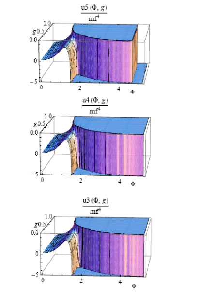
Figure 3: The three figures show, from top to bottom, the potentials $u_{5}$, $u_{4}$ and $u_{3}$ dependence on the field $\Phi$ and the coupling $g$, respectively. The potential scale is chosen for a high magnification range (the minima of the surface at fixed $g$ values are very far below the plotted range) in order to evidence the presence of a threshold for the appearing of the minima when the value of $g$ decreases below $g=1$. Note that for $\Phi$ smaller than some units and not to small values of $g$, the three plotted graphs are similar, indicating that the elimination of the highest fifth, and also the next to highest fourth, powers of the field (or, of the logarithm in the original expansion) in defining $u_{4}$ and $u_{3}$ respectively, are not affecting the results in the mentioned region. The circumstance that the exact evaluated contribution has a negative leading term of order five (which makes the result unbounded from below) explains that for the plot of $u_{5}$ the minima disappear for sufficiently small values of $g$. However, the fact that exact potential should be expected to be bounded from below, we consider that supports our assumption about employing the bounded from below approximations of the potential $u_{4}$ in evaluating the Dilaton properties at the small values of $g$ defined by the $GUT$ and $m_{top}$ mass scales.

IV.1 Dilaton field and mass for $m_{f}$ at the $GUT$ scale

Let us consider now that the highest fermion mass $m_{f}$ is given by the $GUT$ mass scale

$$m_{f} = m_{GUT}=5.06773\times 10^{29}\text{cm}^{-1}$$ (103)

$$\equiv 10^{16}\ \text{GeV},$$

which produces for the coupling $g$ the  value

$$g=m_{f}\text{ }\alpha=-\frac{3}{4}\kappa\text{ }m_{GUT}=-0.0030789542773.$$

The potential $u_{4}$ as function of the field $\Phi$ for this particular value of $g$ is shown in  figure  4.   The minimum of the curve determines an estimate for the vacuum value of the Dilaton field given by

$$\Phi_{vac} = 5.8576156\text{ }=\alpha\text{ }\varphi_{vac},$$ (104)

$$\text{ }\varphi_{vac} = -\frac{4}{3}{5.8576156}\frac{1}{\kappa}.$$ (105)

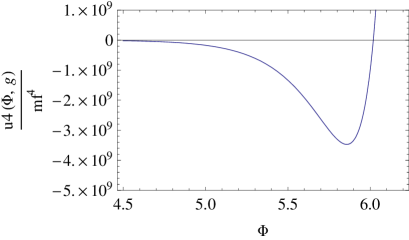
Figure 4: The effective potential $u_{4}$ defined by Eq. 101 as a function of the Dilaton field $\Phi$. The fermion mass was fixed to correspond to the $GUT$ mass $m_{GUT}$ and the renormalization scale $\mu$ was chosen to coincide with this mass. The minimum of the potential is near the value $\Phi=5.7$, which indicates that the field is bound to a high value near the Planck scale.

This result indicates that the  vacuum mean value of the Dilaton field, after assuming that the fermion mass is in the $GUT$ scale, becomes stabilized in the scale of the Planck mass.

Let us consider now the mass of the field excitation.  Its value is determined by the second derivative of the potential curve taken at the minimum, which is given by

$$\left.\frac{d^{2}}{d\Phi^{2}}u_{4}(\Phi,-0.0030789542773)\right|_{\Phi=\Phi^{(m_{GUT})}_{vac}}=1.28179\times 10^{11}m_{f}^{4}.$$ (106)

In order to  estimate the Dilaton mass let us consider the  linearized  equation of motion for the mean field

$$(\frac{1}{\alpha^{2}}\partial^{2}+\left.\frac{d^{2}}{d\Phi^{2}}u_{4}(\Phi,-0.00307895)\right|_{\Phi=\Phi_{vac}^{(m_{GUT})}})\,\Phi=0,$$ (107)

in which the factor $\frac{1}{\alpha^{2}}$ multiplying the   D’Alembertian  appears due to the previously done change of field variable $\Phi=\alpha\,\varphi.$

The above wave equation leads to the dispersion relation for the Dilaton modes

$$(-\frac{1}{\alpha^{2}}p^{2}+\left.\frac{d^{2}}{d\Phi^{2}}u_{4}(\Phi,-0.00307895)\right|_{\Phi=\Phi_{vac}^{(m_{GUT})}})=0,$$ (108)

which for the case of the particle at rest $p=(m_{D}^{(m_{GUT})},0,0,0)$  determines for the Dilaton the mass estimate

$$m_{D}^{(m_{GUT})} = \sqrt{\left.\frac{d^{2}}{d\Phi^{2}}u_{4}(\Phi,-0.00307895)\right|_{\Phi=\Phi_{vac}^{(m_{GUT})}}}m_{GUT}^{2}\mid\alpha\mid$$ (109)

$$= \text{ \ \ }5.58626\times 10^{32}\ \ \ \ \text{\ \ \ cm}^{-1}.$$

Therefore, the predicted order of the mass  for the Dilaton also lays at extremely high values  which  make this field mode undetectable in a direct way.

IV.2 Dilaton mean value and mass for $m_{f}$ at the $top$ quark mass scale

It is also of interest to take as $m_{f}$ the highest currently known fermion mass: that is, the top quark one   

$$m_{top}=172.0\pm 0.9\ \ \ \text{GeV}=8.7164\times 10^{15}\,\ \ \text{cm}^{-1}.$$ (110)

Then, the coupling $g$ in this case takes the small value

$$g=m_{f}\,\alpha=-\frac{3}{4}\kappa\,m_{top}=-5.32659\times 10^{-17}.$$ (111)

Figure 5 shows the dependence of the potential $u_{4}$ as a function of the field $\Phi$ at the above value of the coupling $g$.   The minimum of the curve in this case gives for the mean Dilaton field  at the vacuum

$$\Phi_{vac}^{(m_{top})} = 36.3020096=\alpha\text{ }\varphi_{vac}^{(m_{top})},$$ (112)

$$\text{ }\varphi_{vac}^{(m_{top})} = -\frac{4}{3}{36.3020096}\frac{1}{\kappa}.$$ (113)

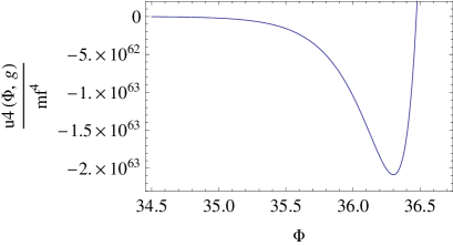
Figure 5: The effective potential $u_{4}$ plotted as a function of the Dilaton field $\Phi$. In this case the coupling was defined by a fermion mass correspond to the top quark one $m_{top}$ and the renormalization scale $\mu$ was also chosen to coincide with this value. The minimum of the potential is now near the value $\Phi=36.7765$, which indicates that the field is again staying at a high value.

This result predicts that, assuming that the maximal fermion mass in Nature is given by the top quark one, which means a lower bound for the physical masses, the vacuum field of  the Dilaton, again becomes stabilized in a scale, which although not being so high, is yet close to the Planck mass.

In this case the dispersion relation for the Dilaton modes takes the form

$$(-\frac{1}{\alpha^{2}}p^{2}+\left.\frac{d^{2}}{d\Phi^{2}}u_{4}(\Phi,-5.32659\times 10^{-17})\right|_{\Phi=\Phi_{vac}^{(m_{top})}})=0.$$ (114)

But, after evaluating for the second derivative of the potential at the minimum to be

$$\left.\frac{d^{2}}{d\Phi^{2}}u_{4}(\Phi,-5.32659\times 10^{-17})\right|_{\Phi=\Phi_{vac}^{(m_{top})}}=6.86404\times 10^{64},$$ (115)

and fixing again the rest frame momentum $p=(m_{D}^{(m_{top})},0,0,0)$  estimates for the Dilaton mass the value

$$m_{D}^{(m_{top})} = \sqrt{\left.\frac{d^{2}}{d\Phi^{2}}u_{4}(\Phi,-5.32659\times 10^{-17})\right|_{\Phi=\Phi_{vac}^{(m_{top})}}}\times m_{top}^{2}\mid\alpha\mid$$ (116)

$$= \text{ }\ 7.07209\times 10^{29}\text{\ \ \ \ \ \ \ \ \ \ \ \ \ \ \ cm}^{-1}.$$

Henceforth, also in this case the predicted mass for the Dilaton turns to be a high value being now close to the $GUT$ scale. Thus, it can be expected that for a maximal fermion mass in Nature ranging between the lower bound $m_{top}$ and the  $GUT$ scale one, the   Dilaton gets stabilized at a large field value as required by string phenomenology. In addition the resulting values of its mass, for the same range of $m_{f}$ masses, is also out of the current observability range of particle detectors.

V Conclusions

The predictions for the Dilaton stabilization problem determined the existence of massive fermion matter had been further investigated here. The fermion field mass values are considered in two cases: the top quark mass representing the lower bound of all existing but yet unknown fermion masses in Nature, and the energy scale of the grand unification theories of order $10^{16}$ GeV. In both situations, the results indicate that the Dilaton mean field becomes stabilized at the very high values required by its role in allowing gravity to have its observed properties. Then, the same existence of matter seems to be a possible source of the dynamical fixation of the Dilaton field at the high values, required by String Theory to imply the observable Einstein theory of gravity.  Furthermore, the evaluations indicate that the Dilaton field is also found to be strongly bound around its mean value, by showing a large mass being close to the $GUT$ or Planck scales. Therefore, the work identifies a possible explanation for the lack of observable consequences of the Dilaton scalar field in Nature. The discussion included  contributions to the effective potential up to 3-loops. This allows to consider the influence of the inclusion of different leading perturbative correction on the main conclusions. After, disregarding in the evaluated potential: a) the highest order term (quintic) in the expansion in powers of $Log(\frac{m}{\mu})$ (which determined the unbounded from below structure of the potential at large $\Phi$  values )  or b) the two highest orders (the quintic and the quartic ones), the obtained modified potentials are both bounded from below at high field values. This procedure allows that minima as functions of $\Phi$ exist for arbitrarily small values of  the coupling $g$. This allows to evaluate the small coupling values associated to the $GUT$ and $top$ quark masses. The fact that the Yukawa theory under consideration should exhibit a bounded from below potential, then supports this here adopted procedure for  estimating the  vacuum mean values and mass of the Dilaton field. However, further higher loop evaluations are convenient to define more precise estimated values of the Dilaton vacuum field and mass and also for checking that they do not affect the picture. The validity of the employed Yukawa like approximation in which the power expansion in Dilaton field of exponential factor of the Fermion mass is limited to the linear term in the field, is argued when the fermion mass is very much smaller than Plank mass.

Appendix A

In this Appendix we discuss two points which improve the argues in the work: a) Adding a discussion about the validity of the Yukawa approximation; and b) To clarify the exposition of the results which indicate the stabilization of the vev and the mass generation.

Below we address the two main critical remarks we identified in the Report:

.1 Yukawa approximation

Let us study the validity of only retaining the linear term in the expansion of the exponential of the Dilaton field multiplying the fermion mass in the action. For this purpose let us consider the mean value of the square of the radiation field  $\phi_{r}$ times the Dilaton coupling $\alpha$ in the just considered Yukawa model.  The square root of this quantity gives a measure of the amount of the quantum fluctuations of $\alpha$ $\phi_{r}(x)$. A resulting small value of this quantity justifies the approximation done in the work. In terms of the Dilaton Green function $D$ this quantity can be written as follows:

$$\langle 0|\text{ }\alpha_{(R)}^{2}\phi_{(R)}^{r2}(x)|0\rangle =\alpha_{(R)}^{2}\int\frac{dp^{d}}{(2\pi)^{d}i}D(p)$$

$$=\alpha_{(R)}^{2}\int\frac{dp^{d}}{(2\pi)^{d}i}\frac{1}{-p^{2}+\Pi(p,m,d)}$$

$$=\alpha_{(R)}^{2}\int\frac{dp_{e}^{d}}{(2\pi)^{d}}\frac{1}{p_{e}^{2}+\Pi(p_{e},m,d)}.$$ (117)

where $\Pi$ is its selfenergy which will be evaluated in the one loop approximation, by excluding the divergent pole parts. This corresponds to using the MS substraction by also employing the Feynman expansion in terms of the renormalized fields incorporating counterterms.

Let us now consider that the bare Dilaton theory being quantized, is valid in the Planck scale where its action is assumed to define a low energy physics for a string theory. Then, after denoting with the B subindex the bare quantities, the relations between the bare and renormalized magnitudes are

$$\alpha_{(B)} =-\frac{3}{4}\kappa=Z_{\alpha}^{\frac{1}{2}}\alpha_{(R)}^{2},$$ (118)

$$\phi_{(B)}^{r}(x) =Z_{\phi}^{\frac{1}{2}}\phi_{(R)}^{r}(x).$$ (119)

We will also assume that the product $\alpha_{(R)}^{2}\phi_{(R)}^{r2}(x)$, after the study of the renormalization properties of the theory, can be chosen as a renormalization group invariant, which determines for the renormalization constants the relation

$$Z_{\alpha}^{\frac{1}{2}}=\frac{1}{Z_{\phi}^{\frac{1}{2}}}.$$

Therefore, the squared deviation of the field can be written in the form

$$\langle 0|\alpha_{(R)}^{2}\phi_{(R)}^{r2}(x)|0\rangle =\frac{\alpha_{(B)}^{2}}{Z_{\phi}}\langle 0|\text{ }\phi_{(R)}^{r2}(x)\text{ }|0\rangle$$

$$=\frac{\alpha_{(B)}^{2}}{Z_{\phi}}\int\frac{dp_{e}^{d}}{(2\pi)^{d}}\frac{1}{p_{e}^{2}+\Pi^{(1)}(p_{e},m,d)}.$$ (120)

Now, in order to get an estimate of this quantity, let us consider the approximation in which the renormalized Yukawa coupling is small and also assume that the finite part of the one loop selfenergy is evaluated at zero momentum. As it will be seen in the comment of the next point, this quantity determines the first approximation for the Dilaton mass as given by the square root of the value of $\ p_{e}^{2}$ fixing the pole of the propagator. As it was mentioned, in the discussion of the next point, assuming that the coupling is small implies that the selfenergy evaluated at zero momentum approximately determines the pole mass of the Dilaton. Thus in this small coupling limit at least the above described approximation can give a reasonable estimate of the field fluctuations.  In addition, as it was supposed in the work, we will fix the scale parameter $\mu$ as coinciding with the fermion mass, that is $\mu=m.$ Therefore, approximating $\Pi^{(1)}(p_{e},m,d)$ by $\Pi^{(1)}(0,m,d)$ and evaluating the remaining simple momentum integral gives

$$\langle 0|\alpha_{(R)}^{2}\phi_{(R)}^{r2}(x)|0\rangle =\frac{\alpha_{(B)}^{2}}{Z_{\phi}}\int\frac{dp_{e}^{d}}{(2\pi)^{d}}\frac{1}{p_{e}^{2}+\Pi^{(1)}(0,m,d)}$$

$$=\frac{\alpha_{(B)}^{2}}{Z_{\phi}}\text{ }\Pi^{(1)}(0,m,d)^{\frac{d-2}{2}}\frac{(\pi)^{2-\epsilon}\Gamma(\epsilon-1)}{(2\pi)^{4-2\epsilon}}.$$ (121)

In order to proceed, let us evaluate the wavefunction renormalization constant $Z_{\phi}$ to further transform the previous formula. The fermion one loop contribution without the substractions is given by the expression

$$\Pi(p,m,d)=-g_{y}^{2}\int\frac{dq^{d}}{(2\pi)^{D}i}Tr[\frac{1}{m-\gamma_{\mu}p^{\mu}}\frac{1}{m-\gamma_{\mu}(p-q)^{\mu}}],$$

to which should be added the wavefunction and mass first order counterterms in order to evaluate $\Pi^{(1)}$ in formula (121). Calculating the Dirac traces and  performing the Wick rotation allows to explicitly determine $\Pi$ as follows

$$\Pi(p_{e},m,D) =-4g_{y}^{2}m^{d-2}\int\frac{dq_{e}^{d}}{(2\pi)^{d}}\frac{1}{1+q_{e}^{2}}+$$

$$g_{y}^{2}\text{ }p_{e}^{2}\int\frac{dq_{e}^{d}}{(2\pi)^{d}}\frac{1}{1+q_{e}^{2}}\frac{1}{1+(p_{e}-q_{e})^{2}}$$

$$=-4g_{y}^{2}\text{ }m^{d-2}\frac{\Gamma(1-\frac{d}{2})}{(2\pi)^{\frac{d}{2}}}+$$

$$g_{y}^{2}\text{ }p_{e}^{2}\frac{m^{-2\epsilon}\Gamma(\epsilon)}{(4\pi)^{\frac{d}{2}}}\int_{0}^{1}dx(1+\frac{p_{e}^{2}}{m^{2}}x(1-x))^{-\epsilon}.$$ (122)

The Feynman parametric integral can be explicitly performed by using the Wolfram Mathematica program in the form

$$\mathcal{F(}\frac{p_{e}^{2}}{m^{2}},\epsilon\mathcal{)} =\int_{0}^{1}dx(1+\frac{p_{e}^{2}}{m^{2}}x(1-x))^{-\epsilon}$$

$$=-\frac{2^{-(1+\epsilon)}(q+\sqrt{q+4})(1-\frac{q}{\sqrt{q^{4}+4}})^{\epsilon}}{q(\epsilon-1)}\times$$

$${}_{2}F_{1}(1-\epsilon,\epsilon,2-\epsilon,\frac{1}{2}(1+\frac{q}{\sqrt{q^{4}+4}}))-$$

$$-\frac{2^{-(1+\epsilon)}(q-\sqrt{q+4})(1+\frac{q}{\sqrt{q^{4}+4}})^{\epsilon}}{q(\epsilon-1)}\times$$

$${}_{2}F_{1}(1-\epsilon,\epsilon,2-\epsilon,\frac{1}{2}(1+\frac{q}{\sqrt{q^{4}+4}})),$$ (123)

$$\operatorname{Re}[\frac{\sqrt{q^{4}+4}}{q} \geq 1]\text{ or }\operatorname{Re}[\frac{\sqrt{q^{4}+4}}{q}\leq 1]\text{ \ or }\frac{\sqrt{q^{4}+4}}{q}\notin\text{real}.$$ (124)

The exact expression for the finite part of the one selfenergy can be obtained by summing the counterterms. This permits to define the  wave function renormalization constant and the coefficient of the mass counterterm as the pole part in $\epsilon$ of the fermion loop contribution. The wavefunction renormalization constant is given as

$$Z_{\phi}=1-\frac{(g_{Y}^{0})^{2}}{(4\pi)^{2}}\frac{1}{\epsilon}.$$

This formula allows to find the limit $d=4-2\,\epsilon\,->4$ limit of the mean of the squared deviation of the field in (121) as follows

$$\langle 0|\alpha_{(R)}^{2}\phi_{(R)}^{r2}(x)|0\rangle =\frac{\alpha_{(B)}^{2}}{Z_{\phi}}\text{ }\Pi^{(1)}(0,m,d)^{\frac{d-2}{2}}\frac{(\pi)^{2-\epsilon}\Gamma(\epsilon-1)}{(2\pi)^{4-2\epsilon}}$$

$$=\alpha^{2}\lim_{\epsilon\rightarrow 0}\frac{\Pi^{(1)}(0,m,d)^{\frac{d-2}{2}}\frac{(\pi)^{2-\epsilon}\Gamma(\epsilon-1)}{(2\pi)^{4-2\epsilon}}}{1-\frac{(g_{Y}^{0})^{2}}{(4\pi)^{2}}\frac{1}{\epsilon}}$$

$$=16\pi^{2}(1-\gamma)\alpha^{2}m^{2}$$

$$=16(\frac{3}{4})^{2}\pi^{2}(1-\gamma)\text{ }\kappa^{2}m^{2},$$ (125)

$$\gamma =0.57721.$$ (126)

This result indicates that the mean squared deviation of the argument of the exponential of the Dilaton radiation field is of the order of the square of ratio between the mass of the fermion and the Planck mass. Therefore, for the values considered in the work: the top quark mass and the GUT unification scale, the exponential interaction term in the Dilaton radiation field should be well approximated by the linear term defining the Yukawa model.

.2 Approximations in determining Dilaton stabilization and mass

In this subsection, we describe the main criteria of stabilization of the vev and the approximations done in evaluating the mass in the paper. Let us consider the definition of the effective action of a scalar field

$$\Gamma[\phi(x)]=\frac{1}{i}\ln Z[j]-\int dx\text{ }j(x)\phi(x),$$

and its expansion around an homogeneous vev $\phi$ in a functional power series in spacetime dependent fluctuation $\varphi(x)$,

$$\Gamma[\phi+\varphi(x)] =\Gamma[\phi]+\int dxj(x)\varphi(x)-\frac{1}{2}\int\int dxdy\varphi(x)D^{-1}(x-y)\varphi(y)+...$$

$$=-V^{(4)}V[\phi]+\int dp\text{ }j^{\ast}(p)\varphi(p)-\frac{V^{(4)}}{2}\int\int\varphi^{\ast}(p)D^{-1}(p)\varphi(p)+...$$

$$=V^{(4)}(V[\phi]+\int dp\text{ }j^{\ast}(p)\varphi(p)-\int\int\varphi^{\ast}(p)D^{-1}(p)\varphi(p)...),$$ (127)

where due to the homogeneity of the vev $\Gamma[\phi]$  is proportional  to the four  dimensional volume $V^{(D)}$. The negative sign in the quadratic in the field term of the expansion comes because the second functional derivative of the effective action respect to the field is the negative of the inverse of the propagator. The quantity $V$ appearing defines the so called effective potential $V[\phi]=-\frac{\Gamma[\phi]}{V^{(4)}}$. The potential $V$ has the interpretation of the  energy density of the quantum system at the value of the also homogeneous external source that sustains it. The stable states of the vev fields are given by the minima of $V$ jona ; coleman .  This property implies that the results in the work indicate the stabilization of the Dilaton vev due to the quantum corrections associated to massive matter fields.

Lets us consider now the question of the approximation in which the results determine an estimation of the mass for the oscillation around the mean field. The discussion in the previous subsection partially helps to clarify this point. The masses of the particles are defined by the squared momenta making equal to zero the inverse propagator

$$D^{-1}(p)=-(p^{2}-\Pi^{(1)}(p,m,4))=0.$$

where, since $\Pi^{(1)}$ is finite, $d=4$ has been substituted. The approximation which is employed to estimate the Dilaton mass in the work is obtained by expanding the proper mass (the squared momentum value)  which makes vanish the inverse propagator, in powers of the coupling constant $g_{Y}$ as follows

$$p^{2}(g_{Y})=\sum_{m=0,1,2...}p_{m}^{2}(g_{Y}^{0})^{2m}.$$

After substituting this series in the inverse propagator, and noting that the inverse propagator for the scalar field is a function of the momentum only through its squared values and that the coupling expansion of the one loop selfenergy $\Pi^{(1)}$ is already of order $(g_{Y}^{0})^{2}$, it follows

$$-p_{0}^{2} =0,$$

$$(-p_{1}^{2}(g_{Y}^{0})^{2}+\Pi(0,m,4)) =0,$$

$$m^{2} =p^{2}=\Pi^{(1)}(0,m,4)+O((g_{Y}^{0})^{4}).$$ (128)

Therefore, in the first approximation, the proper mass is given by the squared root of the zero momentum component of the selfenergy. Further, the selfenergy at zero momentum coincides with the squared root for the second derivative of the effective potential, and this was the criterion employed to evaluate the Dilaton mass in the work. This property, can be seen after expressing the effective action expanded around an assumed minimum and homogeneous field value as follows

$$\Gamma[\phi+\varphi(x)] =\Gamma[\phi(x)]-\frac{1}{2}\int\int dxdy\varphi(x)D^{-1}(x-y)\varphi(y)+...$$

$$=-V^{(4)}V[\phi]-\frac{V^{(4)}\varphi^{2}}{2}\int\int dzD^{-1}(z)+...$$

$$=-V^{(4)}V[\phi]-\frac{V^{(4)}\varphi^{2}}{2}[D^{-1}(p)]_{p=0}+...$$

$$=-V^{(4)}(V[\phi]+\frac{\varphi^{2}}{2}[\Pi(p)]_{p=0}+..)$$

$$=-V^{(4)}(V[\phi]+\frac{\varphi^{2}}{2}\frac{\partial^{2}}{\partial\phi^{2}}V(\phi)+...,)$$ (129)

$$\frac{\partial^{2}}{\partial\phi^{2}}V(\phi) =[\Pi(p)]_{p=0}.$$ (130)