Breaking of self-averaging properties and selection effects in the Luminous Red Galaxies sample

We study the statistical properties of the Luminous Red Galaxies sample from the Sloan Digital Sky Survey. In particular we test, by determining the probability density function (PDF) of galaxy (conditional) counts in spheres, whether statistical properties are self-averaging within the sample. We find that there are systematic differences in the shape of the PDF and in the location of its peak, signaling that there are major systematic effects in the data which make the estimation of volume average quantities unreliable within this sample. We discuss that these systematic effects are related to the fluctuating behavior of the redshift counts which can be originated by intrinsic fluctuations in the galaxy density field or by observational selection effects. The latter possibility implies that more than $20\%$ of the galaxies have not been observed and that such a selection should not be a smooth function of redshift.

1 Introduction

The sample of Luminous Red Galaxies (LRG) (Eisenstein et al., 2001) from the Sloan Digital Sky Survey (SDSS) (York et al., 2000) is considered to be the best sample to study galaxy large scale structures. One of the main features observed in the LRG sample from the final data release of the SDSS (Abazajian et al., 2009), is that the number density as a function of redshift $n(z)$, usually called the “selection function”, presents a complex behavior. Given that, by construction, the LRG sample should be volume-limited (Eisenstein et al., 2001; Zehavi et al., 2005; Kazin et al., 2010) the behavior of $n(z)$ is expected to be constant if galaxy distribution is close to uniform (up to Poisson noise and radial clustering). It is instead observed that the LRG sample $n(z)$ shows an irregular and not constant behavior. An explanation that it is usually given for this result (Zehavi et al., 2005; Kazin et al., 2010), is that the LRG sample is “quasi” volume limited, in that it does not show a constant $n(z)$. Thus, the features in $n(z)$ are absorbed in the properties of a selection function, which is unknown a priori, but that it is defined a posteriori as the difference between an almost constant $n(z)$ and the behavior observed. Clearly this explanation is unsatisfactory as it is given a posteriori and no independent tests have been provided to corroborate the hypothesis that an important observational selection effect occurs in the data, other than the behavior of $n(z)$ itself. Indeed a different possibility is that the behavior of $n(z)$ is determined by intrinsic fluctuations in the distribution of galaxies and not by selection effects.

We note that if (unknown) selection effects are considered to play a major role in this sample, the question that should be addressed concerns the quality of the data. In the original paper by Eisenstein et al. (2001) it is stated that the sample is volume-limited up to $z\sim 0.38$, modulo minor effects due to K+$e$ corrections (i.e. K-corrections and luminosity evolution). To support that this is the case, $n(z)$ was found, in the early SDSS LRG data (see their Figs.12-13), to be close to flat. However Eisenstein et al. (2005), by considering a much larger LRG sample, noted that the comoving number density displays a close to a constant behavior, “although fluctuations are reaching about the $30\%$ peak-to-peak” (see their Fig.1). More recently, by considering the LRG sample with the same selection in magnitude and redshift as the one considered by Eisenstein et al. (2005), but from the final SDSS data release which is larger by a factor $\sim 3$ in volume, Kazin et al. (2010) (see their Fig.1) noted that there are non-negligible variations in $n(z)$, that, as mentioned above, make difficult to consider this sample as a purely volume limited one.

In this paper we determine the probability density function (PDF) of conditional galaxy counts in spheres . In practice we study the statistical properties of the variable $N_{i}(r)$, which is defined to be the number of galaxies in a sphere a radius $r$ centered on the $i^{th}$ galaxy. This has the advantage to provide a characterization of conditional fluctuations which is not affected by the geometrical constraints of the sample as $n(z)$, which instead explores different volumes at different redshifts. In addition, by measuring the PDF in different regions of the sample we can make a clear test to check whether fluctuations are self-averaging inside the sample. This is the fundamental property that fluctuations are required to have when an average quantity is measured in a given sample.

Indeed a spatial average is meaningful, in the sense that it provides an estimation of the ensemble average property of the given statistics, only when fluctuations are stationary inside the sample (Sylos Labini et al., 2009a; Sylos Labini and Baryshev, 2010). The breaking of self-averaging properties can be generally due to two different reasons. On the one hand when a distribution is not statistically translational and/or rotational invariant, then the fluctuation properties depend on the specific position of the volume in which they are measured. For instance, if the distribution is spherically symmetric around a point, then the relevant role is played by the distance $R$ from the center: fluctuations at different distances $R$ have different properties and for this reason any volume average quantity, computed in regions large enough so that statistical properties (i.e., the local density) change significantly, do not give an useful information about the real properties of the distribution. This same situation occurs when a distance-dependent observational selection effect occurs in the data as it can mimic the break of translational invariance.

On the other hand self-averaging properties can be broken when fluctuations, in a given sample, are too extended in space and have too large amplitude (Sylos Labini et al., 2009a, b). For instance when there are a few large scale structures in given volume, or even a single one, which dominates the distribution then it is not possible to get a meaningful estimation of an average quantity at large enough scales in the sample. This occurs precisely because the sample volume is not large enough to average between different large enough structures. This is a systematic effect that sometimes is refereed to as cosmic variance (Yang and Saslaw, 2010) but that is more appropriately defined as breaking of self-averaging properties (Sylos Labini et al., 2009a), as the concept of variance (which involves already the computation of an average quantity) maybe without statistical meaning in the circumstances described above.

The breaking of self-averaging properties was found to occur in several volume-limited samples of the main galaxy sample (MGS) of the DR6-SDSS (Sylos Labini et al., 2009a). Indeed, it was found that at large enough scales, i.e. $r>30$ Mpc/h, the PDF of conditional fluctuations shows systematic differences when it is measured in volumes located in different positions in the sample. That this corresponds to the breaking of self-averaging properties and not the the breaking of statistical isotropy and/or homogeneity (for intrinsic or observational reasons) is shown by two facts. The first is that the difference between the PDF, measured into two volumes located at small and high redshifts, is not systematically the same. That is, sometimes the PDF measured at low redshift is shifted toward smaller values and sometimes toward higher values. As discussed by Sylos Labini and Baryshev (2010) the breaking of statistical translational invariance, as well as the effect of a redshift dependent selection effect, would be signed by a difference in the PDF at low and high redshift always in the same direction. Secondly, when the larger volumes provided by DR7-SDSS was considered (Antal et al., 2009), the PDF did not show the same difference: this is a clear indication that the breaking of self-averaging properties is due to a systematic volume-dependent effect. In addition, when self-averaging properties were found to be satisfied the PDF was found to be nicely fitted by a Gumbel function and its first and second moments, the average conditional density and the conditional variance, were found to have a scaling behavior as a function of distance. All these behaviors mark a clear departure from spatial uniformity (Antal et al., 2009).

In this paper we perform the test for self-averaging in the LRG sample. In Sect.2 we recall the basic statistical elements which we use in the data analysis. The main features of the data are presented in Sect.3 while in Sect.4 we show our results. We discuss our results in Sect.5 by comparing the results obtained here with the ones measured in the SDSS-MGS by Loveday (2004); Sylos Labini et al. (2009a, b); Yang and Saslaw (2010) and in the 2 degree field redshift survey (2dFGRS) by Sylos Labini et al. (2009c, d). In addition we critically consider the measurements of the conditional average density by Hogg et al. (2004), the assumptions entering in the determination of the two-point correlation function (Kazin et al., 2010) and the problem underlying the determination of the so-called baryon acoustic peak (Eisenstein et al., 2005; Kazin et al., 2010; Martínez, et al., 2009; Sylos Labini et al., 2009e). Finally we draw our conclusions in Sect.6.

2 Statistical background

As it was discussed by Sylos Labini et al. (2009a, b); Sylos Labini and Baryshev (2010) a simple test to determine whether a point distribution is self-averaging in a given sample of linear size $R_{s}$ consists in studying the PDF of conditional galaxy counts in spheres ${\cal N}$ (which contains, in principle, information about moments of any order) in sub-samples of linear size $r<R_{s}$ placed in different and non-overlapping spatial regions of the sample (that we call $S_{1},S_{2},...S_{N}$). That the self-averaging property holds is shown by the fact that $P_{S_{i}}({\cal N};r)$ is the same, modulo statistical fluctuations, in the different sub-samples, i.e.,

$$P_{S_{i}}({\cal N};r)\approx P_{S_{j}}({\cal N};r)\;\forall i\neq j\;.$$ (1)

On the other hand, if determinations of $P_{S_{i}}({\cal N},r)$ in different sample regions $S_{i}$ show systematic differences then, as discussed above, the distribution is not self-averaging because of the presence of non-averaged large scale structures or because it not statistically translational and/or rotational invariant (this includes the case in which a redshift dependent observational selection effect is present). When Eq.1 is not found to be satisfied in a given sample then the determinations of the spatial averages are sample-dependent implying that those statistical quantities do not represent the asymptotic properties of the given distribution (Sylos Labini et al., 2009a; Sylos Labini and Baryshev, 2010).

To test self-averaging is necessary to employ statistical quantities that do not require the assumption of spatial homogeneity inside the sample and thus avoid the normalization of fluctuations to the estimation of the sample average (Sylos Labini et al., 2009a). We therefore consider the PDF of the stochastic variable defined by number of points $N_{i}(r)$ contained in a sphere of radius $r$ centered on the $i^{th}$ point. This depends on the scale $r$ and on the spatial position of the $i^{th}$ sphere’s center, namely its radial distance $R_{i}$ from a given origin (in this case the Earth) and its angular coordinates $\@vec{\alpha}_{i}$. Integrating over $\@vec{\alpha}_{i}$ for fixed radial distance $R_{i}$, we obtain that $N_{i}(r)=N(r;R_{i})$ (Sylos Labini et al., 2009a; Antal et al., 2009; Sylos Labini and Baryshev, 2010).

In Antal et al. (2009) we showed that the Gumbel distribution was a good fit to the data of the SDSS-MGS, marking a clear departure from the Gaussian behavior expected for spatially uniform systems. The Gumbel distribution’s PDF, at fixed $r$, is given by (see Antal et al. (2009) and references therein)

$$P(N)=\frac{1}{\beta}\exp\left[-\frac{N-\alpha}{\beta}-\exp\left(-\frac{N-\alpha}{\beta}\right)\right]\;.$$ (2)

The mean and the standard deviation (variance) of the Gumbel distribution (Eq.2), depend on the scale $r$, and are given by

$$\mu=\alpha+\gamma\beta,\quad\sigma^{2}=(\beta\pi)^{2}/6$$ (3)

where $\gamma=0.5772\dots$ is the Euler constant.

3 The data

The sample we consider in this paper is one of the samples prepared by Kazin et al. (2010). In particular we focus on the so-called DR7-Dim, while we do not present results for the other samples, as the one denoted as bright that contains too few galaxies for a reliable statistical analysis.

The metric distance $R(z;\Omega_{m},\Omega_{\Lambda})$ from the redshift has been computed by using the cosmological parameters with values $\Omega_{m}=0.25$ and $\Omega_{\Lambda}=0.75$.

Given that we exclude redshifts $z>0.36$ and $z<0.16$, the distance limits are: $R_{min}=465$ Mpc/h and $R_{max}=1002$ Mpc/h. The limits in R.A $\alpha$ and Dec. $\delta$ considered are chosen in such a way that (i) the angular region does not overlap with the irregular edges of the survey mask and (ii) the sample covers a contiguous sky area. Thus we have chosen: $\alpha_{min}=130^{\circ}$ and $\alpha_{max}=240^{\circ}$; $\delta_{min}=0^{\circ}$ and $\delta_{max}=50^{\circ}$ . The absolute magnitude is constrained in the range $M\in[-23.2,-21.2]$. With these limits we find $N=41833$ galaxies covering a solid angle $\Omega=1.471$ sr.

4 Results

As discussed in Sect.2 we study the statistical properties of the random variable $N_{i}(r)$ measuring the integrated number of points in a sphere of radius $r$ around $i=1...M(r)$ points. The number of points over which it is possible to compute this quantity at the scale $r$, denoted as $M(r)$, depends on the geometrical constraints of the sample as we consider only spheres that are fully enclosed in the sample boundaries (see for details Sylos Labini et al. (2009a)). At fixed $r$ we make an histogram of the $M(r)$ values of $N_{i}(r)$, which thus represents an estimation of the PDF $P(N;r)$ of conditional fluctuations.

In Fig.1 we show the behavior of the number density as a function of distance. There are two main features: (i) a negative slope between $400$ Mpc/h $<r<$ 800 Mpc/h (i.e., $0.16<z<0.28$) and (ii) a positive slope up to a local peak at $r\sim 950$ Mpc/h (i.e., $z\sim 0.34$). Additional features are present as peaks in the $n(r)$ behavior at $r\sim 500$ ($z\sim 0.18$) and $r\sim 650$ Mpc/h ($z\sim 0.23$). Note that if $n(z)$ were constant we would expect a behavior similar to the one shown by the mock sample extracted from the Horizon simulation with the same geometry of the real LRG sample (Kim et al., 2010) (see Fig.1). This implies that, by addressing the behavior of $n(z)$ to unknown selection effects, it is implicitly assumed that the survey has lost more than the $20\%$ (for $n_{0}=1.2\times 10^{-4}$ galaxies for (Mpc/h)^-3 ) of the galaxies for observational problems. This looks improbable (Eisenstein et al., 2001) although a more careful investigation of the problem must be addressed. Note also that the deficit of galaxies would not be explained by a smooth redshift-dependent effect (as it occurs for $z>0.36$ — see Fig.1 of Kazin et al. (2010)) rather the selection must be strongly redshift dependent as the behavior of $n(z)$ is not monotonic. These facts point, but do not proof, toward an origin of the $n(z)$ behavior due to the intrinsic fluctuations in the galaxy distribution.

Figure 1: Number density as a function of distance for the LRG sample and for a mock sample extracted from the Horizon simulations (units are in (Mpc/h)^-3). The blue dashed line decays as $r^{-1}$ and it is plotted as reference.

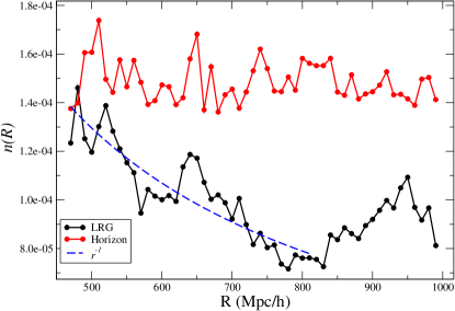
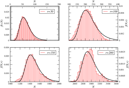
The analysis of fluctuations by studying $n(z)$ shows clearly that the observed behavior is incompatible with model predictions. However the redshift distribution provides only a rough analysis of fluctuations, especially because it is not an average quantity and because it samples different scales differently as the volume in the different redshift bins is not the same. For this reason we determine the statistical properties of the stochastic variable $N_{i}(r)$ previously defined, which allows us to compute the full PDF in sub-samples of equal volume. In Fig.2 we report the PDF at different scales in the LRG sample, together with the best fit with Eq.2, which provides a reasonably good fit. A quantification of the difference of the measured PDF from the Gumbel or Gaussian behaviors is difficult for the problems discussed below.

Figure 2: PDF for $r=50,100,150,200$ Mpc/h together with the best with Eq.2. The number of points contributing to the histogram is respecitively $M(r)=26376,18916,6645,2829$.

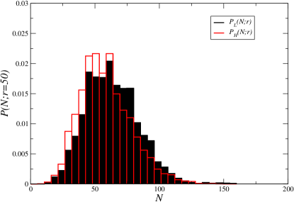
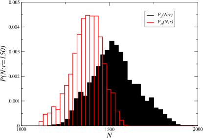
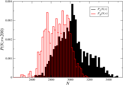
Let us now pass to the self-averaging test described in Sect.2. To this aim we divide the sample into two non-overlapping regions of same volume, one at low (L) redshifts and the other at high (H) redshifts. We then measure the PDF $P_{L}(N;r)$ and $P_{H}(N;r)$ in the two volumes. Given that the total number of points is not very large (i.e., $M(r)\sim 10^{4}$), in order to improve the statistics especially for large sphere radii, we allow a partial overlapping between the two sub-samples, so that galaxies in the L (H) sub-sample counts also galaxies in the H (L) sub-sample. This overlapping clearly can only smooth out differences between $P_{L}(N;r)$ and $P_{H}(N;r)$. Results are shown in Figs.3-6 for $r=50,100,150,200$ Mpc/h respectively. One may note that for $r=50$ Mpc/h the two determinations are much closer than for lager sphere radii for which there is actually a noticeable difference in the whole shape of the PDF . The fact that $P_{H}(N;r)$ is shifted toward smaller values than $P_{L}(N;r)$ is related to the decaying behavior of the redshift counts (see Fig.1): most of the galaxies at low redshifts see a relatively larger local density than the galaxies at higher redshift.

Figure 3: PDF for $r=50$ Mpc/h in the low (L) redshifts and the high (H) redshifts sample. The number of points contributing to the histogram is respecitively for L and H $M(r)=13277,13099$.

Figure 4: As Fig.3 but for $r=100$ Mpc/h. Here $M(r)=7929,7690$.

Figure 5: As Fig.3 but for $r=150$ Mpc/h. Here $M(r)=3495,3150$.

Figure 6: As Fig.3 but for $r=200$ Mpc/h. Here $M(r)=1465,1354$.

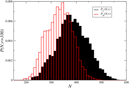
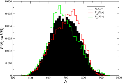
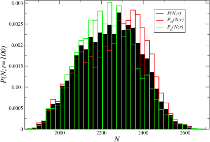
To clarify the features expected in LCDM models, we have done the same analysis in realization of the LRG sample from the Horizon mock samples Kim et al. (2010). In Figs.7-8 we report the PDF computed in the full sample $P(N;r)$ and in the two half-samples $P_{L}(N;r)$ and $P_{H}(N;r)$ as done for the real sample. One may note that the PDF is much more regular and has a bell-shape. Indeed the Gaussian fit is reasonably good. A complementary aspects of these features is provided, as discussed above, by the behavior of the radial density that is almost constant but noisy, where in this case fluctuations are only due to Poisson noise and radial clustering (see Fig.1). These results are clearly expected from a simple theoretical analysis: LCDM models are such that non-linear clustering occurs only at small scales $r<10$ Mpc/h and thus the distribution properties at $\sim 100$ Mpc/h are characterized by Gaussianity, small amplitude fluctuations and weak two-point correlations (see discussion in Sylos Labini et al. (2009a)).

Figure 7: PDF for $r=100$ Mpc/h in the low (L) redshifts and the high (H) redshifts sample for the Horizon mock LRG sample.

Figure 8: PDF for $r=150$ Mpc/h in the low (L) redshifts and the high (H) redshifts sample for the Horizon mock LRG sample.

As a final remark, we note that when applying a random selection to the mock catalog, in such a way to get the same $n(z)$ of the real data, the results of our tests are compatible with the data. Thus, a possible, but as mentioned, unsatisfactory, conclusion is that the LRG is compatible with the mock catalog. We stress again that this conclusion is based on the assumption that an important selection effect, which is not smooth with redshift, occurs in the definition of the sample.

5 Discussion

We have discussed that the number density as a function redshift $n(z)$ of the LRG sample shows, for a wide redshift range, a decreasing behavior as a function of redshift, followed by a sharp increase around $z\sim 0.36$. A different behavior was detected by the $n(z)$ of the bright galaxies in the MGS. In particular Loveday (2004) found that the number density of bright galaxies increases by a factor $\approx 3$ as redshift increases from $z=0$ to $z=0.3$. This is shown, for instance, by the increase of $n(R)$ up tp $z\sim 0.2$ in the two volume limited samples VL4 and VL5 of the MGS shown in Fig.9 (from the Sylos Labini et al. (2009a)). At smaller scales the differential number density shows a fluctuating behavior. To explain the rise of the differential number density in the deepest samples, which contain in average the brightest galaxies of the MGS, a significant evolution in the luminosity and/or number density of galaxies at redshifts $z<0.3$ as been invoked (Loveday, 2004). On the other hand, Sylos Labini et al. (2009a) by measuring the PDF of galaxy counts in spheres, concluded that the volume-limited samples of the MGS, extracted from the SDSS sixth data release, are characterized by the breaking of self-averaging properties for scales $r>30$ Mpc/h and that the increase in the bright galaxies number density is interpreted as an effect due to large scale inhomogeneities.

Figure 9: Radial density in the volume limited samples of the MGS (from Sylos Labini et al. (2009a)) and in the LRG sample. the $n(z)$ for the MGS volume limited samples has been normalized by taking into account the different selection in luminosity in the different samples while for the LRG units are arbitrary.

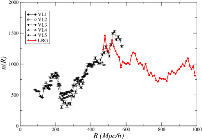
In addition, for galaxies with magnitudes around $M^{*}$ it was subsequently shown by Antal et al. (2009) that self-averaging properties are verified when the larger volumes of the final data release of SDSS is considered. This actually poofs that the breaking of self-averaging properties is due to a finite volume effect and not to galaxy evolution (Sylos Labini and Baryshev, 2010). Moreover in the deeper samples, containing the brightest galaxies, self-averaging properties were found not to be satisfied even in the SDSS final data release (Sylos Labini and Baryshev, 2010). In that case, in agreement with Loveday (2004), it was observed a growth of radial density rather than a decrease. In summary, these behaviors support the conclusion that galaxies from the MGS of the SDSS are not compatible with spatial homogeneity at scales $\sim 100$ Mpc/h. A similar conclusion was drawn from the analysis of the 2dFGRS by Sylos Labini et al. (2009c, d). Recently Yang and Saslaw (2010) found that cosmic variance in the SDSS causes the counts-in-cells distributions in different quadrants to differ from each other by up to 20%, a result which corroborate the results discussed here.

We note that the same systematic effects discussed for the behavior of conditional fluctuations similarly affect the determinations of the two-point correlation function and clearly the detection of the so-called baryon acoustic oscillations (Eisenstein et al., 2005; Kazin et al., 2010; Martínez, et al., 2009). It was indeed shown by Sylos Labini et al. (2009e) that major systematic effects are present in the estimators of $\xi(r)$ and that the variance estimated from the sample itself is much larger than the one deduced from the analysis of mock catalogs, making the detection of the baryon acoustic oscillations statistically unreliable.

Instead of investigating the origin of the fluctuating behavior of $n(z)$, Kazin et al. (2010) focused their attention on the effect of the radial counts on the determination of the two-point correlation function $\xi(r)$. In particular, they proposed mainly two different tests to study what is the effect of $n(z)$ on the determination of $\xi(r)$. The first test consists in taking a mock LRG sample, constructed from a cosmological N-body simulation of the LCDM model, and by applying a redshift selection which randomly excludes points in such a way that the resulting distribution has the same $n(z)$ of the real sample. Then one can compare $\xi(r)$ obtained in the original mock and in redshift-sampled mock. Kazin et al. (2010) find that there is a good agreement between the two. This shows that the particular kind of redshift-dependent random sampling considered for the given distribution, does not alter the determination of the correlation function. In other words this shows that, under the assumption that the observed LRG sample is a realization of the mock LCDM simulation, the $n(z)$ does not affect the result. However, if we want to test whether the LRG sample has the same statistical properties of the mock catalog, we cannot clearly proof (or disproof) this hypothesis by assuming a priori that this is true.

The second test consists in computing $\xi(r)$ in the data, by using a pair-counting method which measures two-point correlations by using a random distribution as reference and by comparing the number of data-data pairs with the number of data-random and/or random-random pairs (Davis and Peebles,, 1983; Landay and Szalay, 1993). Then, to include the variations of $n(z)$ in the data one considers a random sample that is not a purely Poisson distribution. Instead, the random sample is generated so that it has the same $n(z)$ behavior as in the data. This means that in each redshift shell at distance $z$ and of thickness $\Delta z$ the distribution is Poisson with the same density $n(z)$ as observed. This test shows only that a random sample modified in such a way, does not alter the determination of $\xi(r)$ (as it is found by Kazin et al. (2010)). Instead, it does not show that the features in the observed $n(z)$ behavior are taken into account by the fact that the random sample has the same features in the redshift counts.

The behavior of the average conditional properties is clearly ill-defined as long as self-averaging properties are not found to be stable: indeed the average conditional density is just the first moment of the PDF. In Sylos Labini et al. (2009a) we have discussed that up to $\sim 30$ Mpc/h the average conditional density shows approximately a $\sim r^{-1}$ behavior, while in Antal et al. (2009) we find that there is an apparent change of slope at larger scales where the average conditional density decays as $\sim r^{-0.3}$ approximately up to $100$ Mpc/h. A change of slope at $\sim 30$ Mpc/h from $\sim r^{-1}$ was found by Hogg et al. (2004) in a preliminary sample of the LRG. However they claimed that a clear transition to a flat behavior, signaling uniformity, was reached at $\sim 70$ Mpc/h. With the present data, which represent an improvement of almost a factor 3 in volume with respect to the data considered by Hogg et al. (2004), because of the breaking of self-averaging properties, we are not able to make a reliable determination of the average conditional density at scales of the order of $\sim 100$ Mpc/h. However, we note that our results are not compatible with a transition to uniformity at those scales.

6 Conclusions

The number density as a function of redshift in the final LRG sample from the SDSS (Kazin et al., 2010) shows an irregular and mainly decaying behavior which cannot be simply explained by a smooth redshift-dependent selection. We have discussed that the behavior of $n(z)$ is closely related to the properties of fluctuations in this sample. We conclude that these are not self-averaging and thus they do not allow us to make a precise statement on the behavior of volume average quantities, as the average conditional density or the two-point correlation function. Either the behavior of $n(z)$ is determined by intrinsic fluctuations in the LRG distribution which are in amplitude and spatial extension much larger than the ones expected in LCDM models, or there are major observational selection effects intervening in the definition of the LRG sample. For this reason we conclude that forthcoming galaxy samples, as the data from the Baryon Oscillation Spectroscopic Survey (White el al., 2010), with more controlled selection effects, will hopefully clarify the situation.