MPP-2010-151

$W^{\mp}H^{\pm}$ production and CP asymmetry at the LHC

DAO Thi Nhung, Wolfgang HOLLIK and LE Duc Ninh

Max-Planck-Institut für Physik (Werner-Heisenberg-Institut),
D-80805 München, Germany

1 Introduction

The discovery of charged Higgs bosons at the running Large Hadron Collider (LHC) would be unambiguous evidence for new physics. Important mechanisms to produce $H^{\pm}$ include $gb\to tH^{-}$; $q\bar{q},gg\to H^{+}H^{-}$ and $b\bar{b},gg\to W^{\pm}H^{\mp}$ (see [1] for a review and references). The first and the last channel are of particular interest since they allow to search for CP-violating effects at the LHC associated with physics beyond the Standard Model. Recently, the CP-violating asymmetry for $tH^{-}/\bar{t}H^{+}$ production has been calculated in [2].

There have been many discussions devoted to the $pp\to W^{\pm}H^{\mp}$ processes in the Minimal Supersymmetric Standard Model (MSSM) over the last two decades. These studies assume that all the soft supersymmetry-breaking parameters are real and hence CP violation is absent. The two main partonic processes are $b\bar{b}$ annihilation and the loop-induced $gg$ fusion. The first study [3] computed the tree-level $b\bar{b}$ contribution and the $gg$ process with third-generation quarks in the loops using $m_{b}=0$ approximation. This calculation was then extended for finite $m_{b}$, thus allowing the investigation of the process for arbitrary values of $\tan\beta$ (the ratio $v_{2}/v_{1}$ of the vacuum expectation values of the two Higgs doublets) [4, 5]. The inclusion of the squark-loop contribution to the $gg$ channel was done in [6, 7]. The next-to-leading order (NLO) corrections to the $b\bar{b}$ annihilation are more complicated and not complete as yet; the full NLO electroweak (EW) corrections are still missing. The Standard Model QCD (SM-QCD) corrections were calculated in [8, 9], the supersymmetric-QCD (SUSY-QCD) corrections in [10, 11], and the Yukawa part of the electroweak corrections in [12]. There are also studies on the experimental possibility of observing $W^{\mp}H^{\pm}$ production at the LHC with subsequent hadronic $H^{-}\to\bar{t}b$ decay [13] and leptonic $H^{-}\to\tau^{-}\bar{\nu_{\tau}}$ decay [14, 15].

The aim of this paper is multifold. First, we extend the calculation for $pp\to W^{\pm}H^{\mp}$ to the MSSM with complex parameters (complex MSSM, or cMSSM). Second, the full NLO EW corrections to the $b\bar{b}$ annihilation channel are calculated and consistently combined with the other contributions to provide the complete NLO corrections to the $pp\to W^{\pm}H^{\mp}$ processes. Third, CP-violating effects arising in the cMSSM are discussed. The important issues related to the neutral Higgs mixing and large radiative corrections to the bottom-Higgs couplings are also systematically addressed.

In the cMSSM, new sources of CP violation are associated with the phases of soft-breaking parameters and of the Higgsino-mass parameter $\mu$. Through loop contributions, CP violation also enters the Higgs sector, which is CP conserving at lowest order (see for example [16] for more details and references). As a consequence, the $h$, $H$ and $A$ neutral Higgs bosons in general mix and form the mass eigenstates $h_{1,2,3}$ with both CP even and odd properties, which can have important impact on many physical observables.

The bottom-Higgs Yukawa couplings are subject to large quantum corrections in the MSSM. We use the usual QCD running bottom-quark mass to absorb large QCD corrections to the LO results. The potentially large SUSY-QCD corrections, in the large $\tan\beta$ limit, are included into the quantity $\Delta m_{b}$, which is complex in the cMSSM and can be resummed (Section 2.1).

The paper is organized as follows. Section 2 is devoted to the subprocess $b\bar{b}\to W^{\pm}H^{\mp}$, including the issues of effective bottom-Higgs couplings and neutral Higgs mixing. The calculation of the $gg$ fusion part is shown in Section 3. Hadronic cross sections and CP-violating asymmetry are defined in Section 4. Numerical results are presented in Section 5 and conclusions in Section 6. Feynman diagrams, counterterms, and renormalization constants can be found in the Appendices.

2 The subprocess $\boldmath{b\bar{b}\to W^{\mp}H^{\pm}}$

Figure 1: Tree-level diagrams for the partonic process $b\bar{b}\to W^{\pm}H^{\mp}$. $h_{i}$ with $i=1,2,3$ denote the neutral Higgs bosons $h$, $H$ and $A$, respectively.

At the tree level, there are four Feynman diagrams including three $s$-channel diagrams with a neutral Higgs exchange and a $t$-channel diagram, as shown in Fig. 1. The tree-level bottom-Higgs couplings read as follows,

$$\lambda_{b\bar{b}h} = \frac{iem_{b}}{2s_{W}M_{W}}\frac{{\sin{\alpha}}}{{\cos{\beta}}}(P_{L}+P_{R}),$$

$$\lambda_{b\bar{b}H} = \frac{-iem_{b}}{2s_{W}M_{W}}\frac{{\cos{\alpha}}}{{\cos{\beta}}}(P_{L}+P_{R}),$$

$$\lambda_{b\bar{b}A} = \frac{em_{b}}{2s_{W}M_{W}}{\tan{\beta}}(P_{L}-P_{R}),$$

$$\lambda_{b\bar{t}H^{+}} = \frac{ie}{\sqrt{2}s_{W}M_{W}}\left(\frac{m_{t}}{{\tan{\beta}}}P_{L}+m_{b}{\tan{\beta}}P_{R}\right),$$

$$\lambda_{t\bar{b}H^{-}} = \frac{ie}{\sqrt{2}s_{W}M_{W}}\left(m_{b}{\tan{\beta}}P_{L}+\frac{m_{t}}{{\tan{\beta}}}P_{R}\right),$$ (1)

where $P_{L,R}=(1\mp\gamma_{5})/2$, $s_{W}=\sin\theta_{W}$, and $\alpha$ is the tree-level mixing angle of the two CP-even Higgs bosons. In order to obtain reliable predictions, two important issues related to the bottom-Higgs Yukawa couplings and the neutral Higgs mixing have to be addressed. These quantities can get large radiative corrections as will be detailed in the next two sections.

2.1 Bottom-Higgs couplings

In the context of the MSSM, the bottom-Higgs couplings can get large SM-QCD, SUSY-QCD and EW corrections. These large universal corrections can be absorbed into the bottom-Higgs couplings in two steps. First, the SM-QCD corrections are absorbed by using the running bottom-quark mass at one-loop order via

$$m_{b}\longrightarrow m_{b}^{\overline{\text{DR}}}(\mu_{R})=m_{b}\left[1-\frac{\alpha_{s}}{\pi}\left(\frac{5}{3}-\ln\frac{m_{b}^{2}}{\mu_{R}^{2}}\right)\right].$$ (2)

We note, in passing, that the relation between the pole mass and the ${\overline{\text{MS}}}$ mass is different

$$m_{b}^{{\overline{\text{MS}}}}(\mu_{R})=m_{b}\left[1-\frac{\alpha_{s}}{\pi}\left(\frac{4}{3}-\ln\frac{m_{b}^{2}}{\mu_{R}^{2}}\right)\right].$$ (3)

It can be proved that by using the running bottom-quark mass in Eq. (1) the SM-QCD one-loop corrections are independent of $\alpha_{s}\ln(m_{b}^{2})$ [17]. We will therefore replace $m_{b}=m_{b}^{\overline{\text{DR}}}(\mu)$ in Eq. (1). $m_{b}^{\overline{\text{DR}}}$ can be related to the QCD-${\overline{\text{MS}}}$ mass $\overline{m}_{b}(\overline{m}_{b})$, which is extracted from experimental data and is usually taken as an input parameter, at two-loop order as follows [18]

$$m_{b}^{\overline{\text{DR}}}(\mu_{R})=m_{b}^{{\overline{\text{MS}}}}(\mu_{R})\left[1-\frac{\alpha_{s}}{3\pi}-\frac{\alpha_{s}^{2}}{144\pi^{2}}(73-3n)\right],$$ (4)

where $n$ is the number of active quark flavours and the ${\overline{\text{MS}}}$ running mass is evaluated with the two-loop formula

$$m_{b}^{\overline{\text{MS}}}(\mu_{R})=\begin{cases}U_{6}(\mu_{R},m_{t})U_{5}(m_{t},\overline{m}_{b})\overline{m}_{b}(\overline{m}_{b})\quad&\text{for}\quad\mu_{R}>m_{t}\\ U_{5}(\mu_{R},\overline{m}_{b})\overline{m}_{b}(\overline{m}_{b})\quad&\text{for}\quad\mu_{R}\leq m_{t}\end{cases}$$ (5)

where the evolution factor $U_{n}$ reads (see e.g. [19])

$$U_{n}(Q_{2},Q_{1}) = \left(\frac{\alpha_{s}(Q_{2})}{\alpha_{s}(Q_{1})}\right)^{d_{n}}\left[1+\frac{\alpha_{s}(Q_{1})-\alpha_{s}(Q_{2})}{4\pi}J_{n}\right],\quad Q_{2}>Q_{1}$$

$$d_{n} = \frac{12}{33-2n},\quad J_{n}=-\frac{8982-504n+40n^{2}}{3(33-2n)^{2}}.$$ (6)

The second step is to absorb large universal SUSY-QCD and EW corrections into the couplings in Eq. (1). This is achieved by using the following effective bottom-Higgs couplings [19, 20, 21, 22]:

$$\bar{\lambda}_{b\bar{b}h} = \frac{iem_{b}^{\overline{\text{DR}}}}{2s_{W}M_{W}}\frac{{\sin{\alpha}}}{{\cos{\beta}}}\left(\Delta_{b}^{1}P_{L}+\Delta_{b}^{1*}P_{R}\right),$$

$$\bar{\lambda}_{b\bar{b}H} = \frac{-iem_{b}^{\overline{\text{DR}}}}{2s_{W}M_{W}}\frac{{\cos{\alpha}}}{{\cos{\beta}}}(\Delta_{b}^{2}P_{L}+\Delta_{b}^{2*}P_{R}),$$

$$\bar{\lambda}_{b\bar{b}A} = \frac{em_{b}^{\overline{\text{DR}}}}{2s_{W}M_{W}}{\tan{\beta}}(\Delta_{b}^{3}P_{L}-\Delta_{b}^{3*}P_{R}),$$

$$\bar{\lambda}_{b\bar{t}H^{+}} = \frac{ie}{\sqrt{2}s_{W}M_{W}}\left(\frac{m_{t}}{{\tan{\beta}}}P_{L}+m_{b}^{\overline{\text{DR}}}{\tan{\beta}}\Delta_{b}^{3*}P_{R}\right),$$

$$\bar{\lambda}_{t\bar{b}H^{-}} = \frac{ie}{\sqrt{2}s_{W}M_{W}}\left(m_{b}^{\overline{\text{DR}}}{\tan{\beta}}\Delta_{b}^{3}P_{L}+\frac{m_{t}}{{\tan{\beta}}}P_{R}\right),$$ (7)

where

$$\Delta_{b}^{1} = \frac{1-\Delta_{b}/({\tan{\beta}}{\tan{\alpha}})}{1+\Delta_{b}},$$

$$\Delta_{b}^{2} = \frac{1+\Delta_{b}{\tan{\alpha}}/{\tan{\beta}}}{1+\Delta_{b}},$$

$$\Delta_{b}^{3} = \frac{1-\Delta_{b}/({\tan{\beta}})^{2}}{1+\Delta_{b}}.$$ (8)

The leading corrections proportional to ${\cal{O}}(\alpha_{s}{\tan{\beta}},\alpha_{t}{\tan{\beta}},\alpha{\tan{\beta}})$ with $\alpha_{t}=h_{t}^{2}/(4\pi)$ and $h_{t}$ being the superpotential top coupling are included in $\Delta m_{b}$ [19]. This quantity is UV finite and can be calculated by considering the one-loop corrections to the $H_{2}^{0}b\bar{b}$ coupling (which is zero at tree level) where $H_{2}^{0}$ is the neutral component of the second Higgs doublet. It can also be extracted from the one-loop bottom-quark self-energy [23, 24]. In the cMSSM, we find

$$\Delta m_{b} = \Delta m_{b}^{SQCD}+\Delta m_{b}^{SEW},$$

$$\Delta m_{b}^{SQCD} = \frac{2\alpha_{s}(Q)}{3\pi}M_{3}^{*}\mu^{*}\tan\beta\;I(m_{\tilde{b}_{1}}^{2},m_{\tilde{b}_{2}}^{2},m_{\tilde{g}}^{2}),\quad Q=(m_{\tilde{b}_{1}}+m_{\tilde{b}_{2}}+m_{\tilde{g}})/3,$$

$$\Delta m_{b}^{SEW} = \Delta m_{b}^{\tilde{H}\tilde{t}}+\Delta m_{b}^{\tilde{W}}+\Delta m_{b}^{\tilde{B}},$$

$$\Delta m_{b}^{\tilde{H}\tilde{t}} = \frac{\alpha_{t}}{4\pi}A_{t}^{*}\mu^{*}\tan\beta\;I(m_{\tilde{t}_{1}}^{2},m_{\tilde{t}_{2}}^{2},|\mu|^{2})$$

$$\Delta m_{b}^{\tilde{W}} = -\frac{\alpha}{8\pi s_{W}^{2}}M_{2}^{*}\mu^{*}{\tan{\beta}}\big{[}2|U_{11}^{\tilde{t}}|^{2}I(m_{\tilde{t}_{1}}^{2},|M_{2}|^{2},|\mu|^{2})+2|U_{21}^{\tilde{t}}|^{2}I(m_{\tilde{t}_{2}}^{2},|M_{2}|^{2},|\mu|^{2})$$

$$+|U_{11}^{\tilde{b}}|^{2}I(m_{\tilde{b}_{1}}^{2},|M_{2}|^{2},|\mu|^{2})+|U_{21}^{\tilde{b}}|^{2}I(m_{\tilde{b}_{2}}^{2},|M_{2}|^{2},|\mu|^{2})\big{]}$$

$$\Delta m_{b}^{\tilde{B}} = -\frac{\alpha}{72\pi c_{W}^{2}}M_{1}^{*}\mu^{*}{\tan{\beta}}\big{[}3(|U_{11}^{\tilde{b}}|^{2}+2|U_{12}^{\tilde{b}}|^{2})I(m_{\tilde{b}_{1}}^{2},|M_{1}|^{2},|\mu|^{2})$$ (9)

$$+3\,(2|U_{22}^{\tilde{b}}|^{2}+|U_{21}^{\tilde{b}}|^{2})I(m_{\tilde{b}_{2}}^{2},|M_{1}|^{2},|\mu|^{2})+2I(m_{\tilde{b}_{1}}^{2},m_{\tilde{b}_{2}}^{2},|M_{1}|^{2})\big{]},$$

with the auxiliary function

$$I(a,b,c)=-\frac{1}{(a-b)(b-c)(c-a)}\left(ab\ln\frac{a}{b}+bc\ln\frac{b}{c}+ca\ln\frac{c}{a}\right).$$ (10)

$M_{1}$, $M_{2}$, $M_{3}$ (each with a phase $M_{j}=|M_{j}|e^{i\phi_{j}}$) and $\mu=|\mu|e^{i\phi_{\mu}}$ are the bino ($\tilde{B}$), wino ($\tilde{W}$), gluino ($\tilde{g}$) and Higgsino ($\tilde{H}$) mass parameters, respectively. $A_{f}=|A_{f}|e^{i\phi_{f}}$, here $f$ means fermion, denotes the soft supersymmetry-breaking trilinear scalar coupling. $\tilde{b}_{i}$ and $\tilde{t}_{i}$ with $i=1,2$ are the sbottom and stop mass eigenstates, respectively. $U^{\tilde{b}}$ and $U^{\tilde{t}}$ are $2\times 2$ mixing matrices. By setting all the phases to zero we obtain the results for the real MSSM (rMSSM), which agree with those given in [25, 19]. Since we are also interested in the effect of the $A_{b}$ phase, corrections proportional to $A_{b}$ are resummed by [26, 20]

$$\Delta_{b} = \frac{\Delta m_{b}}{1+\Delta_{1}},$$

$$\Delta_{1} = -\frac{2\alpha_{s}(Q)}{3\pi}M_{3}^{*}A_{b}I(m_{\tilde{b}_{1}}^{2},m_{\tilde{b}_{2}}^{2},m_{\tilde{g}}^{2}).$$ (11)

We remark that $\Delta_{b}$ is complex and depends on $\phi_{\mu}$, $\phi_{f}$, $\phi_{i}$ with $i=1,2,3$. The effective couplings in Eq. (7) are used in the calculations of the tree-level, SM-QCD and SUSY-QCD contributions to the $b\bar{b}\to W^{\mp}H^{\pm}$ process and the $gg$ fusion. For the NLO EW corrections we use the tree-level couplings Eq. (1) with $m_{b}=m_{b}^{\overline{\text{DR}}}(\mu_{R})$.

In the explicit one-loop calculations, we have to subtract the $\Delta_{b}$-related corrections which have already included into the tree-level contribution to avoid double counting. This can be done by adding the following counterterms

$$\delta m_{b}^{h} = m_{b}^{\overline{\text{DR}}}\left(1+\frac{1}{{\tan{\alpha}}{\tan{\beta}}}\right)(\Delta_{b}P_{L}+\Delta_{b}^{*}P_{R}),$$

$$\delta m_{b}^{H} = m_{b}^{\overline{\text{DR}}}\left(1-\frac{{\tan{\alpha}}}{{\tan{\beta}}}\right)(\Delta_{b}P_{L}+\Delta_{b}^{*}P_{R}),$$

$$\delta m_{b}^{A} = m_{b}^{\overline{\text{DR}}}\left[1+\frac{1}{({\tan{\beta}})^{2}}\right](\Delta_{b}P_{L}-\Delta_{b}^{*}P_{R}),$$

$$\delta m_{b}^{H^{+}} = m_{b}^{\overline{\text{DR}}}\left[1+\frac{1}{({\tan{\beta}})^{2}}\right]\Delta_{b}^{*}P_{R},$$

$$\delta m_{b}^{H^{-}} = m_{b}^{\overline{\text{DR}}}\left[1+\frac{1}{({\tan{\beta}})^{2}}\right]\Delta_{b}P_{L}$$ (12)

to $\delta m_{b}$ in the corresponding bottom-Higgs-coupling counterterms, as listed in Appendix B. Moreover, Eq. (12) is used with $\Delta_{b}=$ $\Delta m_{b}^{SQCD}$, $\Delta m_{b}^{SEW}$ for the SUSY-QCD and EW corrections, respectively.

2.2 Neutral Higgs-boson propagators

In the MSSM, the neutral Higgs boson masses are subject to large radiative corrections in particular from the Yukawa sector of the theory. As a consequence, the tree-level Higgs masses can be quite different from the physical ones. This important effect should be considered in the NLO calculations of processes with intermediate neutral Higgs exchange.

In our calculation, both subprocesses include $s$-channel diagrams with internal neutral Higgs bosons, (Fig. 1 and Fig. 20). For $b\bar{b}\to W^{\mp}H^{\pm}$ there is also a $t$-channel diagram at tree level which gives the dominant contribution at high energies. Thus, the higher-order corrections to the internal Higgs propagators are not expected to have important effects in this subprocess at high energies. This will be verified in our numerical studies in Section 5.3. The situation is different with the $gg$ fusion since the $s$-channel (triangle) contribution is large. The higher-order corrections to the internal Higgs propagators can therefore be significant in this case, as will be confirmed in Section 5.5. This issue has not been addressed in the previous studies.

In a general amplitude with internal neutral Higgs bosons that do not appear inside loops, the structure describing the Higgs-exchange part of an amplitude is given by

$${\cal{A}}(p^{2})=\sum_{ij}\Gamma_{i}\,\Delta_{ij}(p^{2})\,\Gamma_{j},\quad i=h,H,A,$$ (13)

where $\Gamma_{i,j}$ are one-particle irreducible Higgs vertices. $p$ is the momentum in the Higgs propagator, which is given in terms of the $3\times 3$ propagator matrix

$$\Delta(p^{2}) = i[p^{2}-{\mathbf{M}}(p^{2})]^{-1},$$

$${\mathbf{M}}(p^{2}) = \begin{pmatrix}m_{h}^{2}-\hat{\Sigma}_{hh}(p^{2})&-\hat{\Sigma}_{hH}(p^{2})&-\hat{\Sigma}_{hA}(p^{2})\\ -\hat{\Sigma}_{hH}(p^{2})&m_{H}^{2}-\hat{\Sigma}_{HH}(p^{2})&-\hat{\Sigma}_{HA}(p^{2})\\ -\hat{\Sigma}_{hA}(p^{2})&-\hat{\Sigma}_{HA}(p^{2})&m_{A}^{2}-\hat{\Sigma}_{AA}(p^{2})\end{pmatrix}.$$ (14)

$m_{i}$ ($i=h,H,A$) are the lowest-order Higgs-boson masses, and $\hat{\Sigma}_{ij}$ the renormalized self-energies. The physical masses can be found by diagonalizing the above matrix [27]. By using this propagator matrix we effectively resum all the one-loop corrections to the neutral Higgs self-energies.

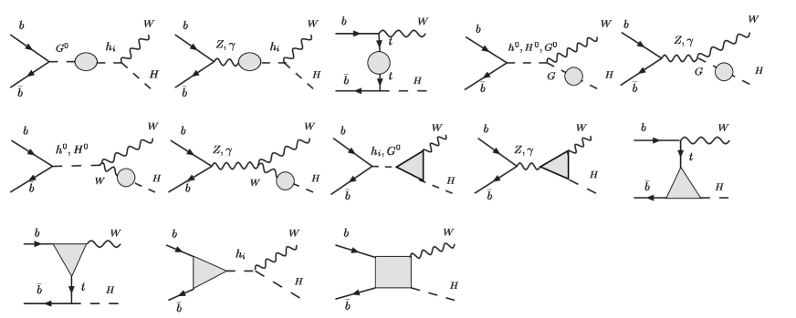
Figure 19: One-loop EW contributions for the partonic process $b\bar{b}\to W^{\mp}H^{\pm}$. The shaded regions are the one-particle irreducible vertices. The diagrams are drawn with Jaxodraw [61].

In our calculation, we keep the full propagator matrix and Eq. (13) whenever neutral Higgs-bosons are exchanged connecting three-point vertices in the tree-level $b\bar{b}$ contributions and in the $gg$ fusion diagrams. As a consequence, when including the NLO EW corrections, we have to discard all Feynman diagrams containing diagonal and nondiagonal $h_{i}h_{j}$ self-energies to avoid double counting (see Fig. 19). Whenever neutral Higgs bosons appear inside a loop, the tree-level expressions are used for propagators and couplings.

The renormalized Higgs self-energies in Eq. (14) are calculated at NLO by using the hybrid on-shell and $\overline{\text{DR}}$ scheme (see Section 2.6 and [27] for details). Our results have been successfully checked against the ones of FeynHiggs [27, 28, 29, 30]. It is noted that FeynHiggs has the option to include the leading two-loop ${\cal{O}}(\alpha_{s}\alpha_{t})$ corrections in the cMSSM [31, 32]. We have verified that the effects of these two-loop corrections are negligible in our numerical analysis and we thus chose to perform the numerical evaluation with the one-loop self-energies.

To quantify the effect of the neutral Higgs propagators we introduce two approximations for the subprocess $b\bar{b}\to W^{\mp}H^{\pm}$: The improved-Born approximation (IBA) including both the $\Delta_{b}$ resummation and the neutral Higgs mixing resummation, and the simpler version IBA1 which contains only the resummed $\Delta_{b}$ together with tree-level Higgs boson masses and couplings. By LO we refer to the tree-level $b\bar{b}\to W^{\mp}H^{\pm}$ contribution with $m_{b}=m_{b}^{\overline{\text{DR}}}(\mu_{R})$ and the tree-level Higgs sector.

2.3 SM-QCD corrections

The NLO contribution includes the virtual and real gluonic corrections. The virtual corrections, displayed by the Feynman graphs in Fig. 16, contain an extra gluon in the loops. The calculation is done by using the technique of constrained differential renormalisation (CDR) [33] which is, at one-loop level, equivalent to regularization by dimensional reduction [34, 35]. We have also checked by explicit calculations that it is also equivalent to dimensional regularization [36] in this case.

Concerning renormalization, the bottom-quark mass appearing in the Yukawa couplings is renormalized by using the $\overline{\text{DR}}$ scheme. It means that the running $m_{b}^{\overline{\text{DR}}}(\mu_{R})$ (see Section 2.1) is used in the Yukawa couplings and the one-loop counterterm reads

$$\delta m_{b}^{\overline{\text{DR}}}=-m_{b}\frac{C_{F}\alpha_{s}}{4\pi}3C_{UV},$$ (15)

where $C_{F}=4/3$, $C_{UV}=1/\varepsilon-\gamma_{E}+\ln(4\pi)$ in $D=4-2\varepsilon$ space-time dimensions with $\gamma_{E}$ denoting Euler’s constant. The bottom-quark mass related to the initial state (in the kinematics $p_{b,\bar{b}}^{2}=m_{b}^{2}$ and the spinors) is treated as the pole mass since the correct on-shell (OS) behavior must be assured. Indeed the $m_{b}^{{\text{OS}}}$ effect here is very small and can be neglected. As mentioned in Section 2.1, the final results are independent of $\ln(m_{b}^{{\text{OS}}})$. We will therefore set $m_{b}^{{\text{OS}}}=m_{b}^{\overline{\text{DR}}}(\mu_{R})$ everywhere in this paper. The finite wave-function normalization factors for the bottom quarks can be taken care of by using the OS scheme for the wave-function renormalization. For the top quark, the pole mass is used throughout this paper. Accordingly, the mass counterterm is calculated by using the OS scheme (Appendix B).

The real QCD corrections consist of the processes with external gluons,

$$b+\bar{b} \to W^{-}+H^{+}+g,$$

$$b+g \to b+H^{+}+W^{-},$$

$$\bar{b}+g \to \bar{b}+W^{-}+H^{+},$$ (16)

corresponding to the Feynman diagrams shown in Fig. 17. For the gluon-radiation process, soft and collinear divergences occur. The soft singularities cancel against those from the virtual corrections, while the collinear singularities are regularized by the bottom-quark mass. The gluon–bottom-induced processes are infrared finite but contain collinear singularities, which are regularized by the bottom-quark mass as well. After adding the virtual and real corrections, the result is collinear divergent and proportional to $\ln(m_{b}^{2}/\hat{s})$, where $\sqrt{\hat{s}}$ is the center-of-mass energy. These singularities are absorbed into the bottom and gluon parton distribution functions (PDF), as discussed in Section 4.

Following the line of [37], we apply both the dipole subtraction scheme [38, 39] and the two-cutoff phase space slicing method [40] to extract the singularities from the real corrections. The two techniques give the same results within the integration errors. However, the error of the dipole subtraction scheme is much smaller than the one of the phase space slicing method. We will therefore use the dipole subtraction scheme in the numerical analysis.

2.4 Subtracting the on-shell top-quark contribution

A special feature of the gluon-induced processes in (16) is the appearance of on-shell top-quarks decaying into $bW$ (and $bH^{+}$ when kinematically allowed), which requires a careful treatment and has been discussed in the previous literature, e.g. in [41, 42, 43]. Our approach is similar to the one described in [41, 42], with the difference that we perform the zero top-quark width limit.

We demonstrate the procedure in terms of the process $\bar{b}g\to W^{-}H^{+}\bar{b}$. The Feynman diagrams (Fig. 17c) include a subclass involving the decay $\bar{t}\to\bar{b}W^{-}$. When the internal $\bar{t}$ can be on-shell, the propagator pole must contain a finite width $\Gamma_{t}$, which is regarded here as a regulator:

$$\frac{i}{q^{2}-m_{t}^{2}}\longrightarrow\frac{i}{q^{2}-m_{t}^{2}+im_{t}\Gamma_{t}}.$$ (17)

This on-shell contribution is primarily a $\bar{t}H^{+}$ production and should therefore not be considered a NLO contribution. For the genuine NLO correction, the on-shell top contribution has to be discarded in a gauge invariant way. Starting from the full set of diagrams, the squared matrix element reads as follows,

$$|M|^{2}=|M_{{\text{OS}}}|^{2}+2\operatorname{Re}[M_{{\text{OS}}}M_{\text{non-OS}}^{*}]+|M_{\text{non-OS}}|^{2},$$ (18)

where the subscripts ${}_{{\text{OS}}}$ and ${}_{\text{non-OS}}$ denote the contribution of the on-shell $\bar{t}$ diagrams and the remainder, respectively. The OS part, differential in the $bW$ invariant mass, to be subtracted can be identified as

$$\frac{d\sigma^{\bar{b}g\to W^{-}H^{+}\bar{b}}}{dM_{bW}^{2}}\bigg{|}_{OS}^{\text{sub}}=\sigma^{\bar{b}g\to H^{+}\bar{t}}{\rm{Br}}(\bar{t}\to\bar{b}W^{-})\frac{m_{t}\Gamma_{t}}{\pi[(M_{bW}^{2}-m_{t}^{2})^{2}+m_{t}^{2}\Gamma_{t}^{2}]},$$ (19)

where ${\rm{Br}}(\bar{t}\to\bar{b}W^{-})=\Gamma_{\bar{t}\to\bar{b}W^{-}}^{LO}/\Gamma_{t}$. The ratio on the right-hand side (rhs) of Eq. (19) approaches $\delta(M_{bW}^{2}-m_{t}^{2})$ when $\Gamma_{t}\to 0$. The subtracted NLO contribution, regularised with the help of $\Gamma_{t}$, can be written in the following way,

$$\sigma^{\bar{b}g\to W^{-}H^{+}\bar{b}}_{\text{reg}}(\Gamma_{t}) = \int dM_{bW}^{2}\left(\frac{d\sigma_{{\text{OS}}}^{\bar{b}g\to W^{-}H^{+}\bar{b}}}{dM_{bW}^{2}}-\sigma^{\bar{b}g\to H^{+}\bar{t}}\frac{m_{t}\Gamma_{t}{\rm{Br}}(\bar{t}\to\bar{b}W^{-})}{\pi[(M_{bW}^{2}-m_{t}^{2})^{2}+m_{t}^{2}\Gamma_{t}^{2}]}\right)$$ (20)

$$+ \sigma^{\bar{b}g\to W^{-}H^{+}\bar{b}}_{\text{inter}}+\sigma^{\bar{b}g\to W^{-}H^{+}\bar{b}}_{\text{non-OS}},$$

where the interference and non-OS terms arise from the second and third terms in Eq. (18).

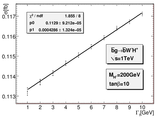
Figure 2: Dependence of the partonic cross section $\sigma^{\bar{b}g\to W^{-}H^{+}\bar{b}}_{\text{reg}}$ on the width regulator $\Gamma_{t}$.

There is strong cancellation between the first term in the rhs of Eq. (20) and the rest after subtraction of the collinear part, which makes the result of Eq. (20) very small, yielding an essentially linear dependence on $\Gamma_{t}$ as displayed in Fig. 2. We can thus perform the limit $\Gamma_{t}\to 0$ and obtain a gauge invariant expression by

$$\sigma^{\bar{b}g\to W^{-}H^{+}\bar{b}}_{\text{reg}}=\lim_{\Gamma_{t}\to 0}\sigma^{\bar{b}g\to W^{-}H^{+}\bar{b}}_{\text{reg}}(\Gamma_{t}).$$ (21)

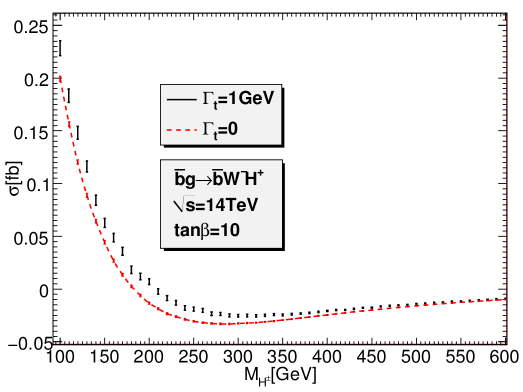
Figure 3: The finite hadronic cross section $\sigma^{\bar{b}g\to W^{-}H^{+}\bar{b}}_{\text{reg}}$ after subtracting the OS top-quark and the collinear-singularity contributions as a function of $M_{H^{\pm}}$.

Fig. 3 shows that the finite gluon-induced contribution obtained in this way at the hadronic level (after proper subtraction of the collinear part) is very small for large values of $M_{H^{\pm}}$, but it can be of some significance when the charged Higgs boson is light.

The method described above is completely analogous for the process $bg\to W^{-}H^{+}b$. For low masses, $M_{H^{\pm}}<m_{t}$, the intermediate on-shell top quark can also decay into $H^{+}b$. This additional OS contribution can be extracted by using the same extrapolation method. For completeness, we list here the expressions for the decay widths of $t\to bW^{+}$ and $t\to bH^{+}$ at lowest order,

$$\Gamma^{LO}_{t\to bW^{+}} =\frac{\alpha}{16m_{t}^{3}M_{W}^{2}s_{W}^{2}}(m_{t}^{2}-M_{W}^{2})^{2}(m_{t}^{2}+2M_{W}^{2}),$$ (22)

$$\Gamma^{LO}_{t\to bH^{+}} =\frac{\alpha}{16m_{t}^{3}M_{W}^{2}s_{W}^{2}}(m_{t}^{2}-M_{H^{\pm}}^{2})^{2}\left[(m_{b}^{\overline{\text{DR}}}\tan\beta)^{2}|\Delta_{b}^{3}|^{2}+\frac{m_{t}^{2}}{\tan^{2}\beta}\right],$$ (23)

where the $b$-quark mass has been neglected.

2.5 SUSY-QCD corrections

The NLO SUSY-QCD contribution consists only of the virtual one-loop corrections, visualized by the Feynman diagrams with gluino loops in Fig. 18. The only divergent part is the top-quark self energy, which is renormalized in the on-shell scheme. As discussed in Section 2.1, large corrections proportional to $\alpha_{s}M_{3}^{*}\mu^{*}\tan\beta$ have been summed up to all orders in the bottom-Higgs couplings included in the IBA. We therefore have to subtract this part from the explicit one-loop SUSY-QCD corrections to avoid double counting.

2.6 Electroweak corrections

The full NLO EW contributions to the processes $b\bar{b}\to W^{\mp}H^{\pm}$ in the cMSSM have not been computed yet. They comprise both virtual and real corrections. For the virtual part, Fig. 19 illustrates the various classes of one-loop Feynman diagrams. As before, the calculation is performed using the CDR technique. We have also worked out all the necessary counterterms in the cMSSM and implemented them in FeynArts-3.4[44, 45]. Explicit expressions for the counterterms can be found in Appendix B. For the Higgs field renormalization and $\tan\beta$, we use the $\overline{\text{DR}}$ renormalization scheme as specified in [27]. Hence, the correct OS behavior of the external $H^{\pm}$ must be ensured by including the finite wave-function renormalization factor [46]

$$\sqrt{Z_{H^{-}H^{+}}}=1-\frac{1}{2}\operatorname{Re}\frac{\partial}{\partial p^{2}}\hat{\Sigma}_{H^{-}H^{+}}(p^{2})\big{|}_{p^{2}=M_{H^{\pm}}^{2}},$$ (24)

where $\hat{\Sigma}_{H^{-}H^{+}}(p^{2})$ is the $H^{\pm}$ renormalized self-energy. The other renormalization constants are determined according to the OS scheme. To make the EW corrections independent of $\ln m_{f}$ from the light fermions $f\neq t$, we use the fine-structure constant at $M_{Z}$, $\alpha=\alpha(M_{Z})$ as an input parameter. This means that we have to modify the counterterm as

$$\delta Z_{e}^{\alpha(M_{Z})} = \delta Z_{e}^{\alpha(0)}-\frac{1}{2}\Delta\alpha(M_{Z}^{2}),$$

$$\Delta\alpha(M_{Z}^{2}) = \frac{\partial\Sigma_{T}^{AA}}{\partial k^{2}}\bigg{|}_{k^{2}=0}-\frac{\operatorname{Re}\Sigma_{T}^{AA}(M_{Z}^{2})}{M_{Z}^{2}},$$ (25)

where the photon self-energy includes only the light fermion contribution, to avoid double counting.

The real EW contributions correspond to the processes with external photons,

$$b+\bar{b} \to W^{-}+H^{+}+\gamma,$$

$$b+\gamma \to b+H^{+}+W^{-},$$

$$\bar{b}+\gamma \to \bar{b}+W^{-}+H^{+},$$ (26)

described by the Feynman diagrams of Fig. 21. They are calculated in the same way as the real QCD corrections, discussed in Section 2.3 and Section 2.4. Naively, we would expect this photon contribution to be much smaller than the one from the gluon, due to the smallness of the EW coupling $\alpha$ and the photon PDF. This is not always true, however, since the photon couples to the $W^{\pm}$ and $H^{\pm}$ as well. The soft singularities are completely cancelled, as in the case of QCD. The EW splitting $\gamma\to H^{+}H^{-}$ (similarly for $\gamma\to W^{+}W^{-}$), on the other side, can introduce large collinear correction in the limit $M_{H^{\pm}}/Q\to 0$, $Q$ is a typical energy scale. The constraint $M_{H}^{\pm}>M_{W}$ prevents those splittings from becoming divergent. We observe, however, that the finite corrections (after subtracting the collinear bottom-photon and the OS top-quark contributions) from the above $\bar{b}\gamma$ process are still larger than the corresponding QCD ones for $M_{H^{\pm}}<200{~{}\text{GeV}}$, e.g. for $M_{H}=150{~{}\text{GeV}}$ and $\sqrt{s}=14{~{}\text{TeV}}$ by a factor of 2. The photon-induced contribution should thus be included in the NLO calculations for $W^{\pm}/H^{\pm}$ production at high energies. This requires the knowledge of the photon density in the proton, which at present is contained in the set MRST2004qed [47] of PDFs.

3 The subprocess $gg\to W^{\mp}H^{\pm}$

The subprocess $gg\to W^{\mp}H^{\pm}$ is loop induced, in the MSSM with quark- and squark-loop contributions. Fig. 20 summarizes the various one-loop Feynman diagrams, which involve three- and four-point vertex functions. Since the (s)quarks are always coupled to a Higgs boson, the one-loop amplitude is proportional to (s)quark-Higgs couplings. The dominant contributions therefore arise from the diagrams with the third-generation (s)quarks. As in [7], the contribution from the first two generations of (s)quarks is neglected in this paper. Compared to the previous work [7], our calculation is improved by using the effective bottom-Higgs couplings and the resummed neutral Higgs propagators. It turns out that these improvements sizably affect both the cross section and CP-violating asymmetry. We have checked our results against those of [7] for the case of the real MSSM using the tree-level couplings and Higgs propagators and found good agreement.

Figure 4: Feynman diagrams that can produce three-point Landau singularities.

We notice an interesting feature related to the anomalous thresholds. Fig. 1b of [7] shows a very sharp peak close to the normal $t\bar{t}$ threshold. Careful observation reveals that the peak position is slightly above $2m_{t}$ and is obviously more singular than the normal thresholds in Fig. 1a of [7]. This is indeed an anomalous threshold corresponding to the three-point Landau singularity (see [48, 49] and references therein) of the triangle and box diagrams in Fig. 4. A simple calculation following [48] yields the peak position at

$$\hat{s}_{\text{peak}} = \frac{1}{2m_{b}^{2}}\big{[}(M_{H^{\pm}}^{2}+M_{W}^{2})(m_{t}^{2}+m_{b}^{2})-(m_{b}^{2}-m_{t}^{2})^{2}-M_{H^{\pm}}^{2}M_{W}^{2}$$ (27)

$$-\lambda^{1/2}(m_{t}^{2},m_{b}^{2},M_{H_{\pm}}^{2})\lambda^{1/2}(m_{t}^{2},m_{b}^{2},M_{W}^{2})\big{]},$$

with $\lambda(x,y,z)=x^{2}+y^{2}+z^{2}-2(xy+yz+xz)$. The partonic cross section is divergent at $\hat{s}=\hat{s}_{\text{peak}}$ but the result is finite at the hadronic level, i.e. after integrating over $\hat{s}$, since this singularity is logarithmic and thus integrable. The conditions for this anomalous threshold to be in the physical region can also be given [48],

$$2m_{t} \leq \sqrt{\hat{s}}\leq\sqrt{\frac{m_{t}}{m_{b}}[(m_{t}+m_{b})^{2}-M_{W}^{2}]},$$

$$m_{b}+m_{t} \leq M_{H^{\pm}}\leq\sqrt{2(m_{t}^{2}+m_{b}^{2})-M_{W}^{2}}.$$ (28)

Similarly, the three-point Landau singularities can occur in the squark diagrams.

4 Hadronic cross section and CP asymmetry

The LO hadronic cross section, in terms of the LO partonic $b\bar{b}$ annihilation cross section, is given by

$$\sigma^{pp}_{LO}=\int{\rm{d}}x_{1}{\rm{d}}x_{2}[F_{b}^{p}(x_{1},\mu_{F})F_{\bar{b}}^{p}(x_{2},\mu_{F}){\hat{\sigma}}^{b\bar{b}}_{LO}(\alpha^{2},\mu_{R})+(1\leftrightarrow 2)],$$ (29)

where $F_{b/\bar{b}}^{p}(x,\mu_{F})$ is the bottom PDF at momentum faction $x$ and factorization scale $\mu_{F}$. Other $q\bar{q}$-subprocesses ($q=u,d,c,s$) are neglected due to the smallness of light-quark-Higgs couplings.

The NLO hadronic cross section reads as follows,

$$\sigma^{pp}_{NLO} = \sum_{i,j}\frac{1}{1+\delta_{ij}}\int{\rm{d}}x_{1}{\rm{d}}x_{2}[F_{i}^{p}(x_{1},\mu_{F})F_{j}^{p}(x_{2},\mu_{F}){\hat{\sigma}}^{ij}_{NLO}(\alpha^{2},\alpha^{2}\alpha_{s},\alpha^{3},\alpha^{2}\alpha_{s}^{2},\mu_{R})$$ (30)

$$+ (1\leftrightarrow 2)],$$

where $i,j$ = ($b,\bar{b},g,\gamma$) and

$${\hat{\sigma}}^{ij}_{NLO} = {\hat{\sigma}}^{b\bar{b}}_{IBA}(\alpha^{2})+\Delta_{\text{SM-QCD}}{\hat{\sigma}}^{ij}_{NLO}(\alpha^{2}\alpha_{s})+\Delta_{\text{SUSY-QCD}}{\hat{\sigma}}^{ij}_{NLO}(\alpha^{2}\alpha_{s})$$ (31)

$$+ \Delta_{EW}{\hat{\sigma}}^{ij}_{NLO}(\alpha^{3})+{\hat{\sigma}}^{gg}(\alpha^{2}\alpha_{s}^{2})$$

contain the various NLO contributions at the parton level, discussed in the previous sections. As mentioned there, the mass singularities of the type $\alpha_{s}\ln(m_{b})$ and $\alpha\ln(m_{b})$ are absorbed in the quark distributions. We use the MRST2004qed set of PDFs [47], which include ${\cal{O}}(\alpha_{s})$ QCD and ${\cal{O}}(\alpha)$ photonic corrections. As explained in [50], the consistent use of these PDFs requires the ${\overline{\text{MS}}}$ factorization scheme for the QCD, but the DIS scheme for the photonic corrections. We therefore redefine the (anti-)bottom PDF as follows,

$$q(x) = q(x,\mu_{\text{F}}^{2})-\frac{\alpha_{s}C_{F}}{2\pi}\int_{x}^{1}\frac{dz}{z}q\left(\frac{x}{z},\mu_{F}^{2}\right)\bigg{\{}\ln\begin{pmatrix}\frac{\mu_{F}^{2}}{m_{b}^{2}}\end{pmatrix}[P_{qq}(z)]_{+}$$ (32)

$$-\,[P_{qq}(z)(\ln(1-z)^{2}+1)]_{+}+C_{qq}^{{\overline{\text{MS}}}}(z)\bigg{\}}$$

$$-\frac{\alpha Q_{b}^{2}}{2\pi}\int_{x}^{1}\frac{dz}{z}q\left(\frac{x}{z},\mu_{F}^{2}\right)\bigg{\{}\ln\begin{pmatrix}\frac{\mu_{F}^{2}}{m_{b}^{2}}\end{pmatrix}[P_{qq}(z)]_{+}$$

$$-\,[P_{qq}(z)(\ln(1-z)^{2}+1)]_{+}+C_{qq}^{{\text{DIS}}}(z)\bigg{\}}$$

$$-\,\frac{\alpha_{s}T_{F}}{2\pi}\int_{x}^{1}\frac{dz}{z}g\left(\frac{x}{z},\mu_{F}^{2}\right)\bigg{[}\ln\begin{pmatrix}\frac{\mu_{F}^{2}}{m_{b}^{2}}\end{pmatrix}P_{qg}+C_{qg}^{{\overline{\text{MS}}}}(z)\bigg{]}$$

$$-\,\frac{3\alpha Q_{b}^{2}}{2\pi}\int_{x}^{1}\frac{dz}{z}\gamma\left(\frac{x}{z},\mu_{F}^{2}\right)\bigg{[}\ln\begin{pmatrix}\frac{\mu_{F}^{2}}{m_{b}^{2}}\end{pmatrix}P_{q\gamma}+C_{q\gamma}^{{\text{DIS}}}(z)\bigg{]},$$

with $C_{F}=4/3$, $T_{F}=1/2$. The splitting functions are given by

$$P_{qq}(z)=\frac{1+z^{2}}{1-z},\quad P_{qg}(z)=P_{q\gamma}(z)=z^{2}+(1-z)^{2},$$ (33)

and the $[\ldots]_{+}$ prescription is understood in the usual way,

$$\int_{x}^{1}dzf(z)\left[\frac{g(z)}{1-z}\right]_{+}=\int_{x}^{1}dz\frac{[f(z)-f(1)]g(z)}{1-z}-f(1)\int_{0}^{x}dz\frac{g(z)}{1-z}.$$ (34)

Following the standard conventions of QCD, the factorization schemes are specified by

$$C_{qq}^{{\overline{\text{MS}}}}(z) = C_{qg}^{{\overline{\text{MS}}}}(z)=0,$$

$$C_{qq}^{{\text{DIS}}}(z) = \left[P_{qq}(z)\left(\ln(\frac{1-z}{z})-\frac{3}{4}\right)+\frac{9+5z}{4}\right]_{+},$$

$$C_{q\gamma}^{{\text{DIS}}}(z) = P_{q\gamma}\ln(\frac{1-z}{z})-8z^{2}+8z-1.$$ (35)

Having constructed in this way the hadronic cross sections $\sigma(pp\to W^{\pm}H^{\mp})$, we can define the CP-violating asymmetry at the hadronic level in the following way,

$$\delta^{\text{CP }}_{pp} = \frac{\sigma(pp\to W^{-}H^{+})-\sigma(pp\to W^{+}H^{-})}{\sigma(pp\to W^{-}H^{+})+\sigma(pp\to W^{+}H^{-})}.$$ (36)

The numerator gets contributions from the NLO-$b\bar{b}$ corrections (the LO is CP conserving) and the loop-induced $gg$ process. However, the latter is much larger than the former due to the dominant gluon PDF. The CP-violating effect is therefore mainly generated by the $gg$ channel. The LO-$b\bar{b}$ contribution adds only to the CP invariant part and therefore reduces the magnitude of the CP asymmetry.

5 Numerical studies

5.1 Input parameters

We use the following set of input parameters for the SM sector [51, 52],

$$\alpha_{s}(M_{Z}) =0.1197,\quad \alpha(M_{Z}) =1/128.926,$$ (37)

$$M_{W} =80.398{~{}\text{GeV}},\quad M_{Z} =91.1876{~{}\text{GeV}},$$

$$m_{t} =173.1{~{}\text{GeV}},\quad \overline{m}_{b}(\overline{m}_{b}) =4.2{~{}\text{GeV}}.$$

We take here $\alpha_{s}=\alpha_{s}^{{\overline{\text{MS}}}}(\mu_{R})$ at three-loop order [51]. $\overline{m}_{b}(\overline{m}_{b})$ is the QCD-${\overline{\text{MS}}}$ $b$-quark mass, while the top-quark mass is understood as the pole mass. CKM matrix elements are approximated by $V_{td}=V_{ts}=0$ and $V_{tb}=1$.

For the soft SUSY-breaking parameters, we use the adapted CP-violating benchmark scenario (CPX) [53, 54],

$$\begin{aligned} |\mu|&=2{~{}\text{TeV}},|M_{2}|=200{~{}\text{GeV}},\,|M_{3}|=1{~{}\text{TeV}},\,|A_{t}|=|A_{b}|=|A_{\tau}|=900{~{}\text{GeV}},\\ M_{\tilde{Q}}&=M_{\tilde{D}}=M_{\tilde{U}}=M_{\tilde{L}}=M_{\tilde{E}}=M_{\text{SUSY}}=500{~{}\text{GeV}}.\end{aligned}$$ (38)

Since the Yukawa couplings of the first two fermion generations proportional to the small fermion masses are neglected in our calculations, we set $A_{f}=0$ for $f=e,\mu,u,d,c,s$. The values of $M_{1}$ and $M_{2}$ are connected via the GUT relation $|M_{1}|=5/3\tan^{2}\theta_{W}|M_{2}|$. We can set $\phi_{2}=0$ while keeping $\phi_{1}$ as a free parameter. The complex phases of the trilinear couplings $A_{t}$, $A_{b}$, $A_{\tau}$ and the gaugino-mass parameters $M_{i}$ with $i=1,2,3$ are chosen as default according to

$$\phi_{t}=\phi_{b}=\phi_{\tau}=\phi_{3}=\phi_{1}=\frac{\pi}{2},$$ (39)

unless specified otherwise. The phase of $\mu$ is chosen to be zero in order to be consistent with the experimental data of the electric dipole moment. We will study the dependence of our results on $\tan\beta$, $M_{H^{\pm}}$, $\phi_{t}$ and $\phi_{3}$ in the numerical analysis. The $\phi_{b}$ dependence is not very interesting since it is similar to but much weaker than that of $\phi_{t}$.

The scale of $\alpha_{s}$ in the SUSY-QCD resummation of the effective bottom-Higgs couplings Eq. (9) is set to be $Q=(m_{\tilde{b}_{1}}+m_{\tilde{b}_{2}}+m_{\tilde{g}})/3$. If not otherwise specified, we set the renormalization scale equal to the factorization scale, $\mu_{R}=\mu_{F}$, in all numerical results. Our default choice for the factorization scale is $\mu_{F0}=M_{W}+M_{H^{\pm}}$.

Our study is done for the LHC at $7{~{}\text{TeV}}$ and $14{~{}\text{TeV}}$ center-of-mass energy. In the numerical analysis, we will focus on the latter since the total cross section is about an order of magnitude larger. Important results will be shown for both energies.

5.2 Checks on the results

The results in this paper have been obtained by two independent calculations. We have produced, with the help of FeynArts-3.4 and FormCalc-6.0 [35], two different Fortran 77 codes. Loop integrals are calculated by using LoopTools/FF [35, 55]. The phase-space integration is done by using the Monte Carlo integrators BASES [56] and VEGAS [57]. The results of the two codes are in full agreement. On top, we have also performed a number of other checks:

For the process $gg\to W^{\mp}H^{\pm}$, we have verified that the results are QCD gauge invariant. This can be easily done in practice by changing the numerical value of the gluon polarization vector $\epsilon_{\mu}(p,q)$, where $p$ is the gluon momentum and $q$ is an arbitrary reference vector. QCD gauge invariance means that the squared amplitudes are independent of $q$. More details can be found in [58]. As already mentioned, we compared our results also to the ones of [7] for the rMSSM and obtained good agreement.

For the process $b\bar{b}\to W^{\mp}H^{\pm}$, besides the common checks of UV and IR finiteness, we compared our virtual EW corrections to those obtained by using SloopS [59, 60], and the SUSY-QCD corrections to the results of Rauch [11] for the case of vanishing phases. Again, good agreement was found.

5.3 $pp/b\bar{b}\to W^{\mp}H^{\pm}$: LO and improved-Born approximations

In this section, we study the effect of the bottom-Higgs coupling resummation described in Section 2.1 and of the Higgs propagator matrix discussed in Section 2.2.

 

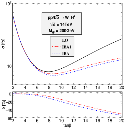
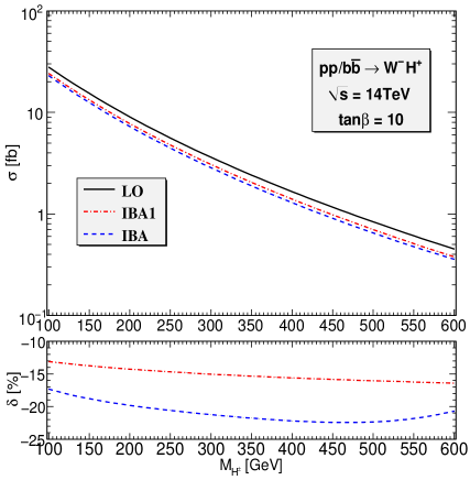
Figure 5: The leading order (LO) cross section with $m_{b}=m_{b}^{\overline{\text{DR}}}$ and the two improved Born approximations (IBA) as functions of $\tan\beta$ (left) and $M_{H^{\pm}}$ (right). $\sigma_{IBA1}$ includes the $\Delta_{b}$ resummation but not the Higgs mixing resummation, while $\sigma_{IBA}$ includes both. The lower panels show the corresponding relative corrections with respect to the LO result.

 

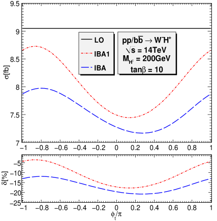
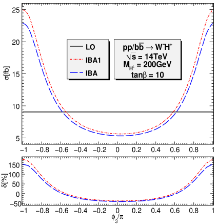
Figure 6: Similar to Fig. 5, but with $\phi_{t}$ (left) and $\phi_{3}$ (right) varied instead.

The results for the approximations IBA and IBA1 defined in section 2.2 are illustrated in Fig. 5 showing the dependence on $\tan\beta$ in the left panel and on the mass $M_{H^{\pm}}$ in the right panel. The relative correction $\delta$, with respect to the LO cross section, is defined as $\delta=(\sigma_{\text{IBA}}-\sigma_{\text{LO}})/\sigma_{\text{LO}}$. For small values of $\tan\beta$ the left-chirality contribution proportional to $m_{t}/\tan\beta$ is dominant while the right-chirality contribution proportional to $m_{b}\tan\beta$ dominates at large $\tan\beta$. The cross section has a minimum around $\tan\beta=8$.

The effect of $\Delta_{b}$ resummation is best understood in terms of Fig. 5 and Fig. 6. The important point is that $\Delta_{b}$ is a complex number and only its real part can interfere with the LO amplitude. Thus, the $\Delta_{b}$ effect is minimum at $\phi_{t,3}=\pm\pi/2$ where the dominant $\Delta m_{b}^{SQCD,\tilde{H}\tilde{t}}$ are purely imaginary and is largest at $\phi_{t,3}=0,\pm\pi$. $\phi_{t}$ enters via EW corrections and $\phi_{3}$ via the SUSY-QCD contributions. Fig. 6 shows that the $\Delta_{b}$ effect can be more than $150\%$. In Fig. 5 where $\Delta_{b}$ is mostly imaginary we see the effect of order ${\cal{O}}(\Delta_{b}^{2})$ which is about $-15\%$ at $\tan\beta=10$. We also observe that the Higgs mixing resummation in the $s$-channel diagrams has a much smaller impact, less than $10\%$, as expected.

5.4 $pp/b\bar{b}\to W^{\mp}H^{\pm}$: full NLO results

 

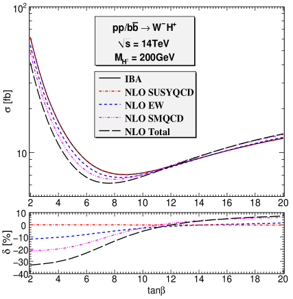
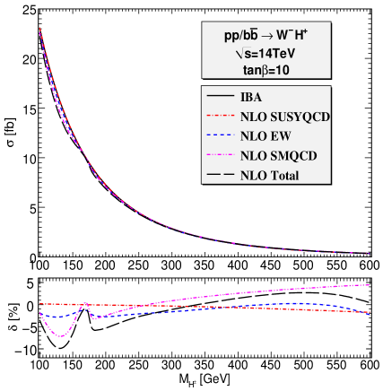
Figure 7: The cross section obtained by using IBA and including various nonuniversal NLO corrections as functions of $\tan\beta$ (left) and $M_{H^{\pm}}$ (right). The lower panels show the corresponding relative corrections to the IBA result.

 

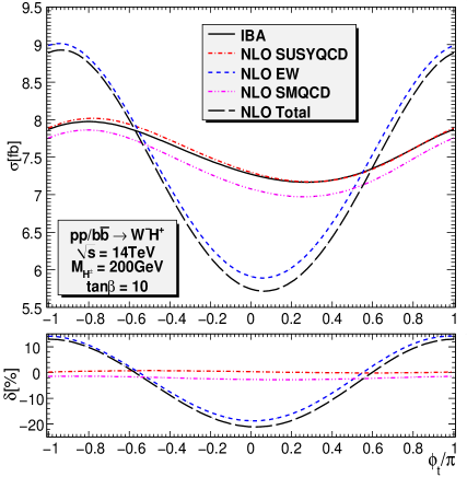
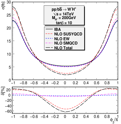
Figure 8: Similar to Fig. 7, but with $\phi_{t}$ (left) and $\phi_{3}$ (right) varied instead.

In this section, we investigate the effects of the SUSY-QCD, SM-QCD, and EW contributions at NLO. As in the previous section, we present here two sets of plots. In Fig. 7 we show the dependence of the total cross sections on $\tan\beta$ and $M_{H^{\pm}}$ at the default CPX phases, in particular $\phi_{t}=\phi_{3}=\pi/2$. As explained above, the ${\cal{O}}(\Delta_{b})$ effect is turned off in this CPX scenario. The SUSY-QCD and EW NLO terms are therefore small at large $\tan\beta$, as shown in Fig. 7 (left). The SM-QCD correction is about $-20\%$ for small $\tan\beta$ and changes the sign around $\tan\beta=11$ due to the competition between the $b\bar{b}$ and the $g$-induced contributions. All the NLO contributions for different values of $\tan\beta$ and $M_{H^{\pm}}$ can be found in Table 1. Fig. 8 shows the dependence of the total cross sections on $\phi_{t}$ and $\phi_{3}$ for $\tan\beta=10$ and $M_{H^{\pm}}=200$GeV. The EW corrections depend strongly on $\phi_{t}$, and the SUSY-QCD corrections on $\phi_{3}$. At $\phi_{t}=\phi_{3}=0,\pm\pi$ the effects are largest. The remaining EW and SUSY-QCD corrections, beyond the ${\cal{O}}(\Delta_{b})$ contribution, are still rather large.

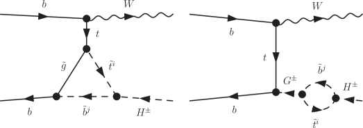
Figure 9: Diagrams that can introduce large SUSY-QCD (left) and EW (right) corrections. $G^{\pm}$ are the charged Goldstone bosons.

In particular, there is the following term of the SUSY-QCD correction,

$$\tilde{\Delta}_{t} = \frac{2\alpha_{s}}{3\pi}M_{3}^{*}\mu^{*}\tan\beta J(m_{\tilde{g}}^{2}),$$

$$J(m^{2}) = |U_{11}^{\tilde{b}}|^{2}|U_{12}^{\tilde{t}}|^{2}I(m^{2},m_{\tilde{t}_{1}}^{2},m_{\tilde{b}_{1}}^{2})+|U_{21}^{\tilde{b}}|^{2}|U_{12}^{\tilde{t}}|^{2}I(m^{2},m_{\tilde{t}_{1}}^{2},m_{\tilde{b}_{2}}^{2})$$ (40)

$$+ |U_{11}^{\tilde{b}}|^{2}|U_{22}^{\tilde{t}}|^{2}I(m^{2},m_{\tilde{t}_{2}}^{2},m_{\tilde{b}_{1}}^{2})+|U_{21}^{\tilde{b}}|^{2}|U_{22}^{\tilde{t}}|^{2}I(m^{2},m_{\tilde{t}_{2}}^{2},m_{\tilde{b}_{2}}^{2}),$$

which can be included in the top-Yukawa part of charged Higgs couplings as follows

$$\tilde{\lambda}_{b\bar{t}H^{+}} = \frac{ie}{\sqrt{2}s_{W}M_{W}}\left(\frac{m_{t}}{{\tan{\beta}}}(1-\tilde{\Delta}_{t})P_{L}+m_{b}^{\overline{\text{DR}}}{\tan{\beta}}\Delta_{b}^{3*}P_{R}\right),$$

$$\tilde{\lambda}_{t\bar{b}H^{-}} = \frac{ie}{\sqrt{2}s_{W}M_{W}}\left(m_{b}^{\overline{\text{DR}}}{\tan{\beta}}\Delta_{b}^{3}P_{L}+\frac{m_{t}}{{\tan{\beta}}}(1-\tilde{\Delta}^{*}_{t})P_{R}\right).$$ (41)

This term originates from the left diagram in Fig. 9 and is important for small $\tan\beta$. This finding agrees with the discussion in [26] where other subleading corrections are also discussed. If the couplings Eq. (41) are used we find that the new-improved LO results move significantly closer to the full NLO results in Fig. 8 (right). The situation in the left part of Fig. 8 is due to the EW corrections. It indicates that there are still large corrections proportional to $A_{t}\mu\alpha_{t}/(4\pi)$ which can be associated with the right diagram in Fig. 9.

The SM-QCD corrections (and EW corrections to a lesser extend) have a striking structure for small masses $M_{H^{\pm}}<m_{t}$ (Fig. 7, right part). This is due to the finite contribution of the process $bg\to W^{-}H^{+}b$. When $M_{H^{\pm}}<m_{t}$ the intermediate top quark can be on-shell and can decay to $H^{+}b$. As discussed in Section 2.4, this OS contribution has to be properly subtracted. The structure indicates that the OS top-quark effect cannot be completely removed and this quantum effect on the $W^{-}H^{+}$ production rate is an interesting feature, which was not discussed in previous studies [8, 9].

5.5 $pp/gg\to W^{\mp}H^{\pm}$: neutral Higgs-propagator effects

 

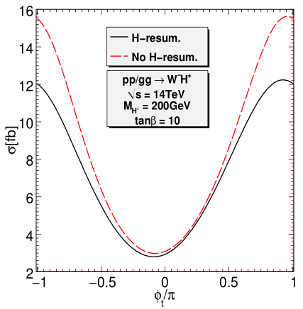
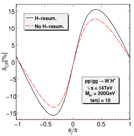
Figure 10: The cross section (left) and CP asymmetry (right) as functions of $\phi_{t}$.

Even though the $gg$-fusion subprocess is loop induced, its contribution can be of the same order as the tree-level $b\bar{b}\to W^{\mp}H^{\pm}$ contribution. Neutral Higgs bosons are exchanged in the $s$-channel and can be described by using effective bottom-Higgs couplings and the full Higgs-propagator matrix. The impact of the latter on the total cross section and CP asymmetry is large as can be seen from Fig. 10. The cross section can be reduced by $20\%$ at $\phi_{t}=\pm\pi$, while the CP asymmetry increases about $25\%$ at $\phi_{t}=\pm\pi/2$. This is consistent with the discussion in Section 2.2. We also observe that the $gg$ contribution is very sensitive to $\phi_{t}$.

5.6 $pp\to W^{\mp}H^{\pm}$: total results at $7{~{}\text{TeV}}$ and $14{~{}\text{TeV}}$

The total production cross section for the $W^{-}H^{+}$ final state at the LHC is shown in Fig. 11 and Fig. 12, as well as in Table 1. The cross section increases by an order of magnitude when the center-of-mass energy goes from $7{~{}\text{TeV}}$ to $14{~{}\text{TeV}}$. The $gg$ contribution is largest for small $\tan\beta$ and large $M_{H^{\pm}}$ while the $b\bar{b}$ dominates when $\tan\beta>12$ and, approximately, $M_{H^{\pm}}<200{~{}\text{GeV}}$. In the right panel of Fig. 11, one can see a little bump on the $gg$ contribution around $M_{H^{\pm}}=200$GeV, attributed to the three-point Landau singularities discussed in Section 3. The total cross section depends strongly on the phases $\phi_{t}$ and $\phi_{3}$ as can be seen from Fig. 12. The $gg$ contribution is almost independent of $\phi_{3}$ since the gluino does not appear at the one-loop level (the contribution through $\Delta_{b}$ resummation is of higher-order effect).

The CP violating asymmetry is shown in Fig. 13 as a function of $\tan\beta$ and $M_{H^{\pm}}$, and in Fig. 14 versus $\phi_{t}$ and $\phi_{3}$. The uncertainty bands obtained by varying the renormalization and factorization scales (we set $\mu_{R}=\mu_{F}$ for simplicity) in the range $\mu_{F0}/2<\mu_{F}<2\mu_{F0}$ are shown only in Fig. 13 since the uncertainty depends strongly on $\tan\beta$ and in particular on $M_{H^{\pm}}$, but not on the phases. A more detailed account of the scale uncertainty of our results is given in the next section. As discussed at the end of Section 4, the CP violating effect is dominantly generated by the gluon-gluon fusion channel. The $b\bar{b}$ channel contributes significantly to the symmetric cross section and thus to the denominator of the CP asymmetry. It is therefore easy to understand why $\delta_{CP}$ is small for large $\tan\beta$ and small $M_{H^{\pm}}$, as seen in Fig. 13. The dependence on $\phi_{3}$ is explained by the same reasons: the numerator is independent of $\phi_{3}$ while the denominator including $\sigma_{b\bar{b}}$ has a minimum at $\phi_{3}=0$. The CP asymmetry is therefore maximum around $\phi_{3}=0$.

Table 1: The total cross section in fb for $pp/bb\to W^{-}H^{+}$ including the IBA and various nonuniversal NLO corrections and for $pp/gg\to W^{-}H^{+}$ at $\sqrt{s}=14{~{}\text{TeV}}$. The charged Higgs-boson masses are given in GeV.

$\tan\beta$	$M_{H^{\pm}}$	$\sigma_{\text{IBA}}$		$\Delta_{\text{EW}}$		$\Delta_{\text{SMQCD}}$		$\Delta_{\text{SUSYQCD}}$		$\sigma_{gg}$		all
5	200	11.	241(1)	-1.	0383(3)	-2.	012(3)	-0.	00821(1)	13.	194(1)	21.	377(3)
10	200	7.	2568(9)	-0.	1989(5)	-0.	178(1)	-0.	00721(2)	7.	9428(5)	14.	815(2)
20	200	12.	546(2)	0.	1881(6)	0.	752(3)	-0.	03570(6)	7.	9968(6)	21.	447(4)
10	150	12.	497(1)	-0.	2574(5)	-0.	561(2)	0.	00191(4)	8.	7064(5)	20.	387(3)
10	400	1.	2907(2)	-0.	00530(7)	0.	0328(2)	-0.	008954(7)	4.	4386(3)	5.	7477(4)
10	600	0.	35740(5)	-0.	00832(2)	0.	01594(5)	-0.	006263(4)	2.	7481(1)	3.	1069(2)

 

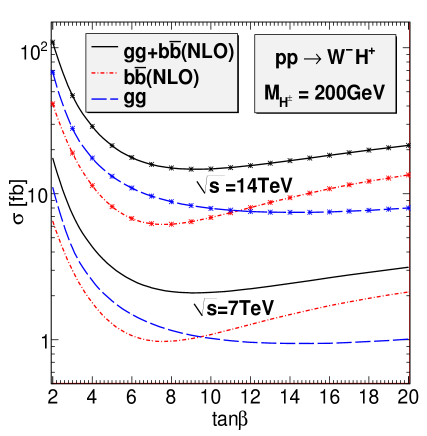
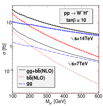
Figure 11: The cross section as a function of $\tan\beta$ (left) and $M_{H^{\pm}}$ (right).

 

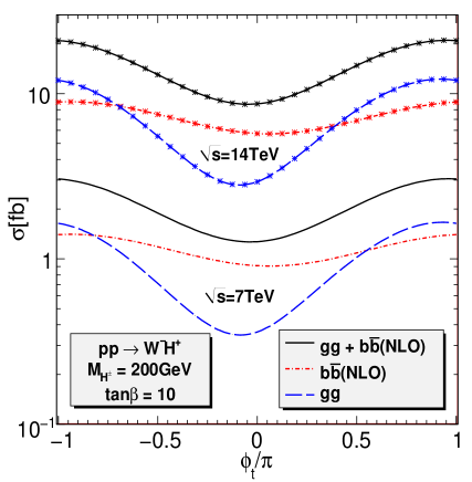
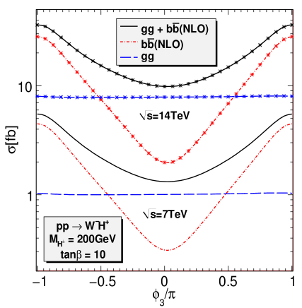
Figure 12: The cross section as a function of $\phi_{t}$ (left) and $\phi_{3}$ (right).

 

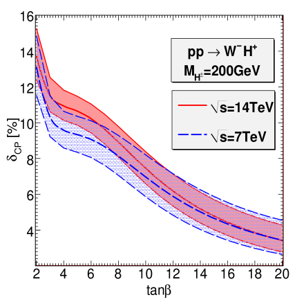
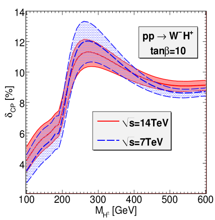
Figure 13: CP asymmetry as a function of $\tan\beta$ (left) and $M_{H^{\pm}}$ (right). Within the band, the scale $\mu_{R}=\mu_{F}$ is varied in the range $\mu_{F0}/2<\mu_{F}<2\mu_{F0}$.

 

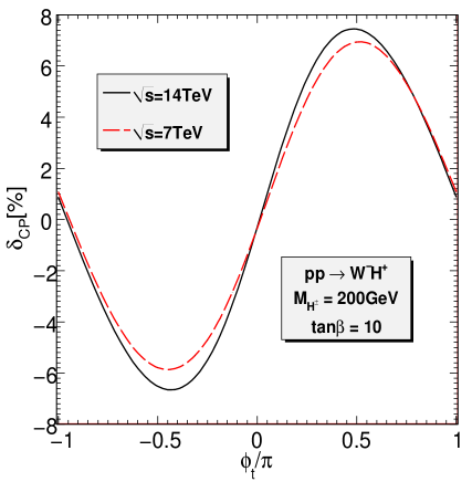
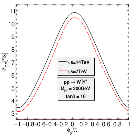
Figure 14: CP asymmetry as a function of $\phi_{t}$ (left) and $\phi_{3}$ (right).

5.7 Scale dependence

 

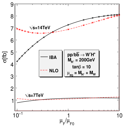
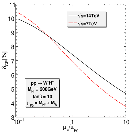
Figure 15: The cross section (left) and CP asymmetry (right) as functions of the renormalization and factorization scales ($\mu_{R}=\mu_{F}$).

In this section we discuss the scale dependence of the total cross sections and CP asymmetries. Since the calculation of the loop-induced subprocess $gg\to W^{\mp}H^{\pm}$ includes only the leading order contribution (with improvements on the bottom-Higgs couplings and neutral Higgs-mixing propagators), there is no cancellation of the renormalization/factorization-scale dependence in this channel. We therefore concentrate on the scale dependence of the $b\bar{b}\to W^{\mp}H^{\pm}$ cross section calculated at NLO, see Fig. 15 (left). We set $\mu_{R}=\mu_{F}$ for simplicity. The remaining uncertainty of the NLO scale dependence is approximately $9\%$ ($9\%$) when $\mu_{F}$ is varied between $\mu_{F0}/2$ and $2\mu_{F0}$, compared to approximately $14\%$ ($7\%$) for the IBA, at $14{~{}\text{TeV}}$ ($7{~{}\text{TeV}}$) center-of-mass energy. The uncertainty is defined as $\delta=[|\sigma(\mu_{F0}/2)-\sigma(\mu_{F0})|+|\sigma(2\mu_{F0})-\sigma(\mu_{F0})|]/\sigma(\mu_{F0})$. The IBA scale dependence looks quite small because we have set both renormalization and factorization scales equal, leading to an “accidental” cancellation. The IBA cross section increases as $\mu_{F}$ increases while it decreases as $\mu_{R}$ increases. We recall that $\mu_{F}$ enters via the bottom-distribution functions and $\mu_{R}$ appears in the running $b$-quark mass. That accidental cancellation depends strongly on the value of $\tan\beta$. We have verified, by studying separately the renormalization and factorization scale dependence, that including NLO corrections does reduce significantly each scale dependence.

Table 2: Cross sections in fb for $pp/b\bar{b}\to W^{-}H^{+}$ and $pp/gg\to W^{-}H^{+}$ at different values of the factorization(renormalization) scale. The CP asymmetries in percentage are also shown.

	$\sqrt{s}=7{~{}\text{TeV}}$								$\sqrt{s}=14{~{}\text{TeV}}$
$\mu_{R}=\mu_{F}$	$\sigma_{\text{IBA}}$		$\sigma^{b\bar{b}}_{\text{NLO}}$		$\sigma^{gg}$		$\delta_{\text{CP}}$		$\sigma_{\text{IBA}}$		$\sigma^{b\bar{b}}_{\text{NLO}}$		$\sigma^{gg}$		$\delta_{\text{CP}}$
$\mu_{F0}/2$	1.	1028(2)	1.	0434(3)	1.	42088(9)	8.	207(8)	6.	6774(8)	6.	633(2)	10.	4606(6)	8.	380(7)
$\mu_{F0}$	1.	1544(1)	1.	0870(2)	1.	02168(6)	6.	967(8)	7.	2568(9)	6.	873(1)	7.	9428(5)	7.	457(8)
$2\mu_{F0}$	1.	1790(1)	1.	1445(2)	0.	7631(5)	5.	868(7)	7.	6648(9)	7.	224(1)	6.	2204(4)	6.	591(8)

Concerning the CP asymmetries, the scale dependence is shown in Fig. 15 (right). We again set here $\mu_{R}=\mu_{F}$. If $\mu_{F}$ is varied between $\mu_{F0}/2$ and $2\mu_{F0}$, the uncertainty is approximately $24\%$ ($34\%$) for $14{~{}\text{TeV}}$ ($7{~{}\text{TeV}}$) center-of-mass energy. This uncertainty is so large because the dominant contribution to the CP asymmetries (the subprocess $gg\to W^{\mp}H^{\pm}$) is calculated only at LO.

In Table 2 we show the values of the cross sections for the two subprocesses as well as the CP asymmetries. The scale-dependence uncertainty of the $gg\to W^{\mp}H^{\pm}$ process is indeed very large. It is mainly due to the running strong coupling $\alpha_{s}(\mu_{R})$ which depends logarithmically on the renormalization scale.

6 Conclusions

In this paper we have studied the production of charged Higgs bosons in association with a $W$ gauge boson at the LHC in the context of the complex MSSM. The NLO EW, SM-QCD and SUSY-QCD contributions to the $b\bar{b}$ annihilation are calculated together with the loop-induced $gg$ fusion. Special care is dedicated to the use of the effective bottom-Higgs couplings and the neutral-Higgs boson propagator matrix. Moreover, the CP violating asymmetry, dominantly generated by the $gg$ fusion parton subprocess, has been investigated. We have shown that the $\Delta_{b}$ and the Higgs-mixing resummations can have large effects on the production rates and CP asymmetry.

Numerical results have been presented for the CPX scenario. It is shown that the production rate and the CP asymmetry depend strongly on $\tan\beta$, $M_{H^{\pm}}$ and the phases $\phi_{t},\phi_{3}$. Large production rates prefer small $\tan\beta$, small $M_{H^{\pm}}$ and the phases $\phi_{t},\phi_{3}$ about $\pm\pi$. Large CP asymmetries occur at small $\tan\beta$, for $M_{H^{\pm}}$ of about $250{~{}\text{GeV}}$, and $\phi_{t}\approx\pm\pi/2$ and $\phi_{3}=0$.

We have also studied the dependence of the results on the renormalization and factorization scales. For the $b\bar{b}$ subprocess, the NLO corrections reduce significantly the scale dependence while the $gg$ fusion suffers from large scale uncertainty mainly due to the running $\alpha_{s}(\mu_{R})$. This makes the final results, in particular the CP asymmetry, depend significantly on the scales. A two-loop calculation would be needed to reduce this uncertainty to the level of a few percents.

Acknowledgments
We are grateful to Fawzi Boudjema for discussions and for sending us the code SloopS. This work was supported in part by the European Community’s Marie-Curie Research Training Network under contract MRTN-CT-2006-035505 ‘Tools and Precision Calculations for Physics Discoveries at Colliders’ (HEPTOOLS).

Appendix A Feynman diagrams

We present here the classes of Feynman diagrams that contribute to the two subprocesses $b\bar{b}\to W^{\mp}H^{\pm}$ and $gg\to W^{\mp}H^{\pm}$. We use $h_{i}$ ($i=1,2,3$) to denote the neutral Higgs bosons ($h,H,A$).

Figure 16: One-loop SM-QCD diagrams for the partonic process $b\bar{b}\to W^{\mp}H^{\pm}$.

(a)

(b)

(c)

Figure 17: Gluon-radiation and gluon-induced QCD diagrams.

Figure 18: One-loop SUSY QCD diagrams for the partonic process $b\bar{b}\to W^{\mp}H^{\pm}$.

Figure 20: One-loop Feynman diagrams for the partonic process $gg\to W^{\mp}H^{\pm}$.

(a)

(b)

(c)

Figure 21: Photon-radiation and photon-induced EW diagrams.

Appendix B Counterterms and renormalization constants

In this section, we list the Feynman rules and counterterms for vertices and propagators which appear in the $b\bar{b}\to W^{\mp}H^{\pm}$ channel. They can be expressed in terms of coupling and field renormalization constants (RC) which relate the bare and renormalized quantities. The RCs are defined as in Ref. [62] for the SM-like fields and as in Ref. [27] for the Higgs sector. The following one-loop Feynman rules use the standard convention and notation of FeynArts [45]. In the vertices all momenta are considered as incoming. We introduce the shorthand notation $s_{\alpha}=\sin\alpha$, $c_{\alpha}=\cos\alpha$, $t_{\alpha}=\tan\alpha$, $s_{\beta}=\sin\beta$, $c_{\beta}=\cos\beta$, $t_{\beta}=\tan\beta$.

Fermion-Fermion-Scalar:

$$\bar{b}bh^{0}: \begin{cases}C^{-}=\frac{s_{\alpha}\,m_{b}}{2c_{\beta}M_{W}s_{W}}\big{(}1+\delta Z_{e}+\frac{\delta m_{b}}{m_{b}}+s^{2}_{\beta}\delta\tan\beta-\frac{\delta M_{W}^{2}}{2M_{W}^{2}}-\frac{\delta s_{W}}{s_{W}}+\frac{1}{2}\delta Z_{hh}\\ \qquad\qquad\qquad\qquad-\frac{1}{2t_{\alpha}}\delta Z_{Hh}+\frac{1}{2}\delta Z_{b,L}+\frac{1}{2}\delta Z_{b,R}^{*}\big{)}\\ C^{+}=\frac{s_{\alpha}\,m_{b}}{2c_{\beta}M_{W}s_{W}}\big{(}1+\delta Z_{e}+\frac{\delta m_{b}}{m_{b}}+s^{2}_{\beta}\delta\tan\beta-\frac{\delta M_{W}^{2}}{2M_{W}^{2}}-\frac{\delta s_{W}}{s_{W}}+\frac{1}{2}\delta Z_{hh}\\ \qquad\qquad\qquad\qquad-\frac{1}{2t_{\alpha}}\delta Z_{Hh}+\frac{1}{2}\delta Z_{b,L}^{*}+\frac{1}{2}\delta Z_{b,R}\big{)}\end{cases}$$

$$\bar{b}bH^{0}: \begin{cases}C^{-}=-\frac{c_{\alpha}\,m_{b}}{2c_{\beta}M_{W}s_{W}}\big{(}1+\delta Z_{e}+\frac{\delta m_{b}}{m_{b}}+s^{2}_{\beta}\delta\tan\beta-\frac{\delta M_{W}^{2}}{2M_{W}^{2}}-\frac{\delta s_{W}}{s_{W}}+\frac{1}{2}\delta Z_{HH}\\ \qquad\qquad\qquad\qquad-\frac{1}{2}t_{\alpha}\delta Z_{hH}+\frac{1}{2}\delta Z_{b,L}+\frac{1}{2}\delta Z_{b,R}^{*}\big{)}\\ C^{+}=-\frac{c_{\alpha}\,m_{b}}{2c_{\beta}M_{W}s_{W}}\big{(}1+\delta Z_{e}+\frac{\delta m_{b}}{m_{b}}+s^{2}_{\beta}\delta\tan\beta-\frac{\delta M_{W}^{2}}{2M_{W}^{2}}-\frac{\delta s_{W}}{s_{W}}+\frac{1}{2}\delta Z_{HH}\\ \qquad\qquad\qquad\qquad-\frac{1}{2}t_{\alpha}\delta Z_{hH}+\frac{1}{2}\delta Z_{b,L}^{*}+\frac{1}{2}\delta Z_{b,R}\big{)}\end{cases}$$

$$\bar{b}bA^{0}: \begin{cases}C^{-}=-i\frac{t_{\beta}\,m_{b}}{2M_{W}s_{W}}\big{(}1+\delta Z_{e}+\frac{\delta m_{b}}{m_{b}}+s^{2}_{\beta}\delta\tan\beta-\frac{\delta M_{W}^{2}}{2M_{W}^{2}}-\frac{\delta s_{W}}{s_{W}}+\frac{1}{2}\delta Z_{AA}\\ \qquad\qquad\qquad\qquad-\frac{1}{2t_{\beta}}\delta Z_{G^{0}A}+\frac{1}{2}\delta Z_{b,L}+\frac{1}{2}\delta Z_{b,R}^{*}\big{)}\\ C^{+}=i\frac{t_{\beta}\,m_{b}}{2M_{W}s_{W}}\big{(}1+\delta Z_{e}+\frac{\delta m_{b}}{m_{b}}+s^{2}_{\beta}\delta\tan\beta-\frac{\delta M_{W}^{2}}{2M_{W}^{2}}-\frac{\delta s_{W}}{s_{W}}+\frac{1}{2}\delta Z_{AA}\\ \qquad\qquad\qquad\qquad-\frac{1}{2t_{\beta}}\delta Z_{G^{0}A}+\frac{1}{2}\delta Z_{b,L}^{*}+\frac{1}{2}\delta Z_{b,R}\big{)}\end{cases}$$

$$\bar{d}_{j}u_{i}H^{-}: \begin{cases}C^{-}=\frac{s_{\beta}}{\sqrt{2}c_{\beta}s_{W}M_{W}}\Big{\{}V_{ij}^{*}\delta m_{d}+V_{ij}^{*}m_{d}(1+\delta Z_{e}-\frac{\delta s_{W}}{s_{W}}+s^{2}_{\beta}\delta\tan\beta-\frac{\delta M_{W}^{2}}{2M_{W}^{2}}\\ \qquad+\frac{1}{2}\delta Z_{H^{-}H^{+}}-\frac{1}{2}\delta Z_{G^{-}H^{+}}/t_{\beta})+\frac{m_{d}}{2}\big{[}2\delta V^{*}_{ij}+\sum_{k}(V^{*}_{ik}\delta Z^{d*}_{kj,R}+V^{*}_{kj}\delta Z^{u}_{ki,L})\big{]}\Big{\}}\\ C^{+}=\frac{c_{\beta}}{\sqrt{2}s_{\beta}s_{W}M_{W}}\Big{\{}V_{ij}^{*}\delta m_{u}+V_{ij}^{*}m_{u}(1+\delta Z_{e}-\frac{\delta s_{W}}{s_{W}}-c^{2}_{\beta}\delta\tan\beta-\frac{\delta M_{W}^{2}}{2M_{W}^{2}}\\ \qquad+\frac{1}{2}\delta Z_{H^{-}H^{+}}+\frac{1}{2}\delta Z_{G^{-}H^{+}}t_{\beta})+\frac{m_{u}}{2}\big{[}2\delta V^{*}_{ij}+\sum_{k}(V^{*}_{ik}\delta Z^{d*}_{kj,L}+V^{*}_{kj}\delta Z^{u}_{ki,R})\big{]}\Big{\}}\par\end{cases}$$

$$\bar{u}_{i}d_{j}H^{+}: \begin{cases}C^{-}=\frac{c_{\beta}}{\sqrt{2}s_{\beta}s_{W}M_{W}}\Big{\{}V_{ij}\delta m_{u}+V_{ij}m_{u}(1+\delta Z_{e}-\frac{\delta s_{W}}{s_{W}}-c^{2}_{\beta}\delta\tan\beta-\frac{\delta M_{W}^{2}}{2M_{W}^{2}}\\ \qquad+\frac{1}{2}\delta Z_{H^{-}H^{+}}+\frac{1}{2}\delta Z_{G^{-}H^{+}}t_{\beta})+\frac{m_{u}}{2}\big{[}2\delta V_{ij}+\sum_{k}(V_{ik}\delta Z^{d}_{kj,L}+V_{kj}\delta Z^{u*}_{ki,R})\big{]}\Big{\}}\\ C^{+}=\frac{s_{\beta}}{\sqrt{2}c_{\beta}s_{W}M_{W}}\Big{\{}V_{ij}\delta m_{d}+V_{ij}m_{d}(1+\delta Z_{e}-\frac{\delta s_{W}}{s_{W}}+s^{2}_{\beta}\delta\tan\beta-\frac{\delta M_{W}^{2}}{2M_{W}^{2}}\\ \qquad+\frac{1}{2}\delta Z_{H^{-}H^{+}}-\frac{1}{2}\delta Z_{G^{-}H^{+}}/t_{\beta})+\frac{m_{d}}{2}\big{[}2\delta V_{ij}+\sum_{k}(V_{ik}\delta Z^{d}_{kj,R}+V_{kj}\delta Z^{u*}_{ki,L})\big{]}\Big{\}}\end{cases}$$

Fermion-Fermion-Vector:

$$\bar{d}_{j}u_{i}W^{-}: C^{-}=-\frac{1}{\sqrt{2}s_{W}}\big{[}V^{*}_{ij}(1+\delta Z_{e}-\frac{\delta s_{W}}{s_{W}}+\frac{1}{2}\delta Z_{W})+\delta V^{*}_{ij}+\frac{1}{2}\sum_{k}(V^{*}_{kj}\delta Z_{ki,L}^{u}+V^{*}_{ik}\delta Z_{kj,L}^{d*})\big{]}$$

$$\bar{u}_{i}d_{j}W^{+}: C^{-}=-\frac{1}{\sqrt{2}s_{W}}\big{[}V_{ij}(1+\delta Z_{e}-\frac{\delta s_{W}}{s_{W}}+\frac{1}{2}\delta Z_{W})+\delta V_{ij}+\frac{1}{2}\sum_{k}(V_{kj}\delta Z_{ki,L}^{u*}+V_{ik}\delta Z_{kj,L}^{d})\big{]}.$$

Scalar-Scalar-Vector:

$$hH^{-}W^{+}: C=-\frac{\cos(\beta-\alpha)}{2s_{W}}\big{[}1+\delta Z_{e}-\frac{\delta s_{W}}{s_{W}}+\frac{1}{2}\delta Z_{WW}+\frac{1}{2}\delta Z_{hh}+\frac{1}{2}\delta Z_{H^{+}H^{-}}$$

$$\qquad\qquad\qquad\qquad-\frac{\sin(\beta-\alpha)}{2\cos(\beta-\alpha)}\big{(}\delta Z_{Hh}-\delta Z_{G^{-}H^{+}})\big{]}$$

$$hH^{+}W^{-}: C=\frac{\cos(\beta-\alpha)}{2s_{W}}\big{[}1+\delta Z_{e}-\frac{\delta s_{W}}{s_{W}}+\frac{1}{2}\delta Z_{WW}+\frac{1}{2}\delta Z_{hh}+\frac{1}{2}\delta Z_{H^{+}H^{-}}$$

$$\qquad\qquad\qquad\qquad-\frac{\sin(\beta-\alpha)}{2\cos(\beta-\alpha)}\big{(}\delta Z_{Hh}-\delta Z_{G^{-}H^{+}})\big{]}$$

$$HH^{-}W^{+}: C=\frac{\sin(\beta-\alpha)}{2s_{W}}\big{[}1+\delta Z_{e}-\frac{\delta s_{W}}{s_{W}}+\frac{1}{2}\delta Z_{WW}+\frac{1}{2}\delta Z_{HH}+\frac{1}{2}\delta Z_{H^{+}H^{-}}$$

$$\qquad\qquad\qquad\qquad-\frac{\cos(\beta-\alpha)}{2\sin(\beta-\alpha)}\big{(}\delta Z_{hH}+\delta Z_{G^{-}H^{+}})\big{]}$$

$$HH^{+}W^{-}: C=-\frac{\sin(\beta-\alpha)}{2s_{W}}\big{[}1+\delta Z_{e}-\frac{\delta s_{W}}{s_{W}}+\frac{1}{2}\delta Z_{WW}+\frac{1}{2}\delta Z_{HH}+\frac{1}{2}\delta Z_{H^{+}H^{-}}$$

$$\qquad\qquad\qquad\qquad-\frac{\cos(\beta-\alpha)}{2\sin(\beta-\alpha)}\big{(}\delta Z_{hH}+\delta Z_{G^{-}H^{+}})\big{]}$$

$$AH^{\pm}W^{\mp}: C=-\frac{i}{2s_{W}}\big{[}1+\delta Z_{e}-\frac{\delta s_{W}}{s_{W}}+\frac{1}{2}\delta Z_{WW}+\frac{1}{2}\delta Z_{AA}+\frac{1}{2}\delta Z_{H^{+}H^{-}}\big{]}$$

$$G^{0}H^{\pm}W^{\mp}: C=-\frac{i}{4s_{W}}(\delta Z_{AG}+\delta Z_{G^{-}H^{+}})$$

Vector-Vector-Scalar:

The vertices $VW^{\mp}H^{\pm}$ with $V=\gamma,Z$ do not appear at tree level. The counterterms are generated at one-loop level, however.

$$\gamma W^{\pm}H^{\mp}: C=\frac{M_{W}}{2}(\delta Z_{G^{-}H^{+}}+\sin{2\beta}\delta\tan\beta),$$

$$ZW^{\pm}H^{\mp}: C=-\frac{M_{W}s_{W}}{2c_{W}}(\delta Z_{G^{-}H^{+}}+\sin{2\beta}\delta\tan\beta).$$ (43)

One also needs counterterms for the renormalized propagators. The complete set of counterterms for the scalar-scalar case can be found in Ref. [27]. We list here extra pieces needed in our calculation.

Scalar-Vector:

Fermion-Fermion:
The renormalization of the fermion fields in the presence of CP violation is a bit more involved than the CP-conserving case. We therefore give here explicit formulae for mass and wave function RCs of the quark fields. The quark self-energy can be decomposed as

$$\Sigma_{q}(p)=p\kern-5.50003pt{/}P_{L}\Sigma_{q,L}(p^{2})+p\kern-5.50003pt{/}P_{R}\Sigma_{q,R}(p^{2})+P_{L}\Sigma_{q,l}(p^{2})+P_{R}\Sigma_{q,r}(p^{2}).$$ (44)

We note that $\Sigma_{q,l}(p^{2})=\Sigma_{q,r}(p^{2})=\Sigma_{q,S}(p^{2})$ in the case of CP invariance. The renormalized self-energy is written as

$$\hat{\Sigma}_{q}(p)= \Sigma_{q}(p)+\tilde{\Sigma}_{q}(p),$$ (45)

$$\tilde{\Sigma}_{q}(p)= \frac{1}{2}(\delta Z_{q,L}+\delta Z_{q,L}^{*})p\kern-5.50003pt{/}P_{L}+\frac{1}{2}(\delta Z_{q,R}+\delta Z_{q,R}^{*})p\kern-5.50003pt{/}P_{L}$$

$$+\frac{m_{q}}{2}(2\frac{\delta m_{q}}{m_{q}}+\delta Z_{q,L}+\delta Z_{q,R}^{*})P_{L}+\frac{m_{q}}{2}(2\frac{\delta m_{q}}{m_{q}}+\delta Z_{q,L}^{*}+\delta Z_{q,R})P_{R}.$$ (46)

In general, $\delta Z_{q,L}$ and $\delta Z_{q,R}$ are complex. $\delta m_{q}$ can always be made real by rephasing the field $\psi_{L}$ (or $\psi_{R}$). At this step any phases can be absorbed into the two factors $\delta Z_{q,L}$ and $\delta Z_{q,R}$ which will have to be determined. It is obvious that the squared amplitude is invariant under a global rephasing

$$\psi=\psi_{L}+\psi_{R}\longrightarrow e^{i\phi_{\psi}}(\psi_{L}+\psi_{R}).$$ (47)

From this freedom we can, for example, make $\delta Z_{q,R}$ real while $\delta Z_{q,L}$ remains complex. We therefore need four conditions to determine the three renormalisation constants. The OS conditions are

$$\operatorname{\widetilde{Re}}\hat{\Gamma}_{q}(p)u(m_{q}) = 0,\quad\left[\frac{1}{p\kern-5.50003pt{/}-m_{q}}\operatorname{\widetilde{Re}}\hat{\Gamma}_{q}(p)\right]u(m_{q})=iu(m_{q}),$$ (48)

$$\operatorname{\widetilde{Re}}\bar{u}(m_{q})\hat{\Gamma}_{q}(p) = 0,\quad\bar{u}(m_{q})\left[\operatorname{\widetilde{Re}}\hat{\Gamma}_{q}(p)\frac{1}{p\kern-5.50003pt{/}-m_{q}}\right]=i\bar{u}(m_{q}),$$ (49)

where $\hat{\Gamma}_{q}(p)=i[p\kern-5.50003pt{/}-m_{q}+\hat{\Sigma}_{q}(p)]$ and $p^{2}=m_{q}^{2}$. $\operatorname{\widetilde{Re}}$ sets the imaginary part of the loop integrals to zero since they are not involved in the renormalisation. The Hermiticity of the Lagrangian imposes[63]

$$\hat{\Gamma}_{q}(p)=-\gamma_{0}^{\dagger}\hat{\Gamma}_{q}^{\dagger}(p)\gamma_{0}.$$ (50)

It is obvious that Eq. (49) can be derived from Eq. (48) and Eq. (50). From these conditions we get the following results

$$\delta m_{q} = \frac{1}{2}\operatorname{\widetilde{Re}}\Big{\{}m_{q}\big{[}\Sigma_{q,L}(m_{q}^{2})+\Sigma_{q,R}(m_{q}^{2})\big{]}+\Sigma_{q,l}(m_{q}^{2})+\Sigma_{q,r}(m_{q}^{2})\Big{\}},$$

$$\delta Z_{q,L} = -\operatorname{\widetilde{Re}}\Big{\{}\Sigma_{q,L}(m_{q}^{2})-\frac{1}{2m_{q}}\big{(}\Sigma_{q,l}(m_{q}^{2})-\Sigma_{q,r}(m_{q}^{2})\big{)}$$

$$+ m_{q}\frac{d}{dp^{2}}\big{[}m_{q}\big{(}\Sigma_{q,L}(p^{2})+\Sigma_{q,R}(p^{2})\big{)}+\Sigma_{q,l}(p^{2})+\Sigma_{q,r}(p^{2})\big{]}_{p^{2}=m_{q}^{2}}\Big{\}},$$

$$\delta Z_{q,R} = -\operatorname{\widetilde{Re}}\Big{\{}\Sigma_{q,R}(m_{q}^{2})-\frac{1}{2m_{q}}\big{(}\Sigma_{q,r}(m_{q}^{2})-\Sigma_{q,l}(m_{q}^{2})\big{)}$$ (51)

$$+ m_{q}\frac{d}{dp^{2}}\big{[}m_{q}\big{(}\Sigma_{q,L}(p^{2})+\Sigma_{q,R}(p^{2})\big{)}+\Sigma_{q,l}(p^{2})+\Sigma_{q,r}(p^{2})\big{]}_{p^{2}=m_{q}^{2}}\Big{\}},$$

where we have used the freedom Eq. (47) to take $\operatorname{Im}(\delta Z_{q,R})=-\operatorname{Im}(\delta Z_{q,L})$. These results agree with the ones in [21].

References

- [1] A. Djouadi, Phys. Rept. 459, 1 (2008), hep-ph/0503173.
- [2] E. Christova, H. Eberl, E. Ginina, and W. Majerotto, Phys. Rev. D79, 096005 (2009), arXiv:0812.4392.
- [3] D. A. Dicus, J. L. Hewett, C. Kao, and T. G. Rizzo, Phys. Rev. D40, 787 (1989).
- [4] A. A. Barrientos Bendezu and B. A. Kniehl, Phys. Rev. D59, 015009 (1999), hep-ph/9807480.
- [5] A. A. Barrientos Bendezu and B. A. Kniehl, Phys. Rev. D61, 097701 (2000), hep-ph/9909502.
- [6] A. A. Barrientos Bendezu and B. A. Kniehl, Phys. Rev. D63, 015009 (2001), hep-ph/0007336.
- [7] O. Brein, W. Hollik, and S. Kanemura, Phys. Rev. D63, 095001 (2001), hep-ph/0008308.
- [8] W. Hollik and S.-h. Zhu, Phys. Rev. D65, 075015 (2002), hep-ph/0109103.
- [9] J. Gao, C. S. Li, and Z. Li, Phys. Rev. D77, 014032 (2008), arXiv:0710.0826.
- [10] J. Zhao, C. S. Li, and Q. Li, Phys. Rev. D72, 114008 (2005), hep-ph/0509369.
- [11] M. Rauch, (2008), arXiv:0804.2428.
- [12] Y.-S. Yang, C.-S. Li, L.-G. Jin, and S. H. Zhu, Phys. Rev. D62, 095012 (2000), hep-ph/0004248.
- [13] S. Moretti and K. Odagiri, Phys. Rev. D59, 055008 (1999), hep-ph/9809244.
- [14] D. Eriksson, S. Hesselbach, and J. Rathsman, Eur. Phys. J. C53, 267 (2008), hep-ph/0612198.
- [15] M. Hashemi, (2010), arXiv:1008.3785.
- [16] E. Accomando et al., (2006), hep-ph/0608079.
- [17] E. Braaten and J. P. Leveille, Phys. Rev. D22, 715 (1980).
- [18] L. V. Avdeev and M. Y. Kalmykov, Nucl. Phys. B502, 419 (1997), hep-ph/9701308.
- [19] M. S. Carena, D. Garcia, U. Nierste, and C. E. M. Wagner, Nucl. Phys. B577, 88 (2000), hep-ph/9912516.
- [20] J. Guasch, P. Hafliger, and M. Spira, Phys. Rev. D68, 115001 (2003), hep-ph/0305101.
- [21] K. E. Williams, PhD thesis, Durham University (2008).
- [22] S. Dittmaier, M. Kramer, M. Spira, and M. Walser, (2009), arXiv:0906.2648.
- [23] S. Heinemeyer, W. Hollik, H. Rzehak, and G. Weiglein, Eur. Phys. J. C39, 465 (2005), hep-ph/0411114.
- [24] L. Hofer, U. Nierste, and D. Scherer, JHEP 10, 081 (2009), arXiv:0907.5408.
- [25] S. Dittmaier, M. Kramer, 1, A. Muck, and T. Schluter, JHEP 03, 114 (2007), hep-ph/0611353.
- [26] M. S. Carena, J. R. Ellis, S. Mrenna, A. Pilaftsis, and C. E. M. Wagner, Nucl. Phys. B659, 145 (2003), hep-ph/0211467.
- [27] M. Frank et al., JHEP 02, 047 (2007), hep-ph/0611326.
- [28] G. Degrassi, S. Heinemeyer, W. Hollik, P. Slavich, and G. Weiglein, Eur. Phys. J. C28, 133 (2003), hep-ph/0212020.
- [29] S. Heinemeyer, W. Hollik, and G. Weiglein, Eur. Phys. J. C9, 343 (1999), hep-ph/9812472.
- [30] S. Heinemeyer, W. Hollik, and G. Weiglein, Comput. Phys. Commun. 124, 76 (2000), hep-ph/9812320.
- [31] S. Heinemeyer, W. Hollik, H. Rzehak, and G. Weiglein, Phys. Lett. B652, 300 (2007), arXiv:0705.0746.
- [32] T. Hahn, S. Heinemeyer, W. Hollik, H. Rzehak, and G. Weiglein, (2010), arXiv:1007.0956.
- [33] F. del Aguila, A. Culatti, R. Munoz Tapia, and M. Perez-Victoria, Nucl. Phys. B537, 561 (1999), hep-ph/9806451.
- [34] W. Siegel, Phys. Lett. B84, 193 (1979).
- [35] T. Hahn and M. Perez-Victoria, Comput. Phys. Commun. 118, 153 (1999), hep-ph/9807565.
- [36] G. ’t Hooft and M. J. G. Veltman, Nucl. Phys. B44, 189 (1972).
- [37] F. Boudjema, L. D. Ninh, S. Hao, and M. M. Weber, Phys. Rev. D81, 073007 (2010), arXiv:0912.4234.
- [38] S. Catani and M. H. Seymour, Nucl. Phys. B485, 291 (1997), [Erratum-ibid. B510, 503 (1998)], hep-ph/9605323.
- [39] S. Dittmaier, Nucl. Phys. B565, 69 (2000), hep-ph/9904440.
- [40] U. Baur, S. Keller, and D. Wackeroth, Phys. Rev. D59, 013002 (1999), hep-ph/9807417.
- [41] W. Beenakker, R. Hopker, M. Spira, and P. M. Zerwas, Nucl. Phys. B492, 51 (1997), hep-ph/9610490.
- [42] T. M. P. Tait, Phys. Rev. D61, 034001 (2000), hep-ph/9909352.
- [43] S. Frixione, E. Laenen, P. Motylinski, B. R. Webber, and C. D. White, JHEP 07, 029 (2008), arXiv:0805.3067.
- [44] T. Hahn, Comput. Phys. Commun. 140, 418 (2001), hep-ph/0012260.
- [45] T. Hahn and C. Schappacher, Comput. Phys. Commun. 143, 54 (2002), hep-ph/0105349.
- [46] W. Hollik and D. T. Nhung, (2010), arXiv:1008.2659.
- [47] A. D. Martin, R. G. Roberts, W. J. Stirling, and R. S. Thorne, Eur. Phys. J. C39, 155 (2005), hep-ph/0411040.
- [48] F. Boudjema and L. D. Ninh, Phys. Rev. D78, 093005 (2008), arXiv:0806.1498.
- [49] L. D. Ninh, PhD thesis, Université de Savoie (2008), arXiv:0810.4078.
- [50] K. P. O. Diener, S. Dittmaier, and W. Hollik, Phys. Rev. D72, 093002 (2005), hep-ph/0509084.
- [51] Particle Data Group, C. Amsler et al., Phys. Lett. B667, 1 (2008).
- [52] Tevatron Electroweak Working Group, (2009), arXiv:0903.2503.
- [53] K. E. Williams and G. Weiglein, Phys. Lett. B660, 217 (2008), arXiv:0710.5320.
- [54] M. S. Carena, J. R. Ellis, A. Pilaftsis and C. E. M. Wagner, Phys. Lett. B495, 155 (2000), arXiv:hep-ph/0009212.
- [55] G. J. van Oldenborgh, Comput. Phys. Commun. 66, 1 (1991).
- [56] S. Kawabata, Comp. Phys. Commun. 88, 309 (1995).
- [57] G. P. Lepage, J. Comput. Phys. 27, 192 (1978).
- [58] F. Boudjema and L. D. Ninh, Phys. Rev. D77, 033003 (2008), arXiv:0711.2005.
- [59] N. Baro, F. Boudjema, and A. Semenov, Phys. Rev. D78, 115003 (2008), arXiv:0807.4668.
- [60] N. Baro and F. Boudjema, Phys. Rev. D80, 076010 (2009), arXiv:0906.1665.
- [61] D. Binosi and L. Theussl, Comput. Phys. Commun. 161, 76 (2004), hep-ph/0309015.
- [62] A. Denner, Fortschr. Phys. 41, 307 (1993), arXiv:0709.1075.
- [63] K. I. Aoki, Z. Hioki, M. Konuma, R. Kawabe, and T. Muta, Prog. Theor. Phys. Suppl. 73, 1 (1982).