Wang-Landau study of the triangular Blume-Capel ferromagnet

Abstract

We report on numerical simulations of the two-dimensional Blume-Capel ferromagnet embedded in the triangular lattice. The model is studied in both its first- and second-order phase transition regime for several values of the crystal field via a sophisticated two-stage numerical strategy using the Wang-Landau algorithm. Using classical finite-size scaling techniques we estimate with high accuracy phase-transition temperatures, thermal, and magnetic critical exponents and we give an approximation of the phase diagram of the model.

1 Introduction

The Blume-Capel model consisting of a spin-one Ising Hamiltonian with a single-ion uniaxial crystal field anisotropy blume ; capel is one of the most studied models in the communities of Statistical Mechanics and Condensed Matter Physics. This is not only because of the relative simplicity with which approximate calculations for this model can be carried out and tested, as well as the fundamental theoretical interest arising from the richness of its phase diagram, but also because versions and extensions of the model can be applied for the description of many different physical structures, some of them being multi-component fluids, ternary alloys, and ³He - ⁴He mixtures lawrie . Noteworthy, latest applications of the Blume-Capel model include analyzes of ferrimagnets, as recently discussed in a thorough contribution by Selke and Oitmaa selke-10 .

The Blume-Capel model is described by the Hamiltonian

$$H=-J\sum_{<ij>}s_{i}s_{j}+\Delta\sum_{i}s_{i}^{2},$$ (1)

where the spin variables $s_{i}$ take on the values $-1,0$, or $+1$, $<ij>$ indicates summation over all nearest-neighbor pairs of sites, and $J>0$ is the ferromagnetic exchange interaction (here we set $J=1$ and $k_{B}=1$ to fix the temperature scale). The parameter $\Delta$ is known as the crystal-field coupling that controls the density of vacancies ($s_{i}=0$). For $\Delta\rightarrow-\infty$ vacancies are suppressed and the model maps onto the Ising model.

As it is well known, the model of equation (1) has been analyzed, besides the original mean-field theory blume ; capel , by a variety of approximations and numerical approaches, mostly on the square lattice. These include the real space renormalization group, Monte Carlo (MC) simulations and MC renormalization-group calculations landau , $\epsilon$-expansion renormalization groups stephen , high- and low-temperature series calculations fox , a phenomenological finite-size scaling analysis using a strip geometry nightingale ; beale , and, finally, the most recent numerical approaches via the Wang-Landau algorithm silva ; hurt ; malakis . The phase diagram of the model consists of a segment of continuous Ising-like transitions at high temperatures and low values of the crystal field which ends at a tricritical point, where it is joined with a second segment of first-order transitions between ($\Delta_{t},T_{t}$) and ($\Delta=zJ/2,T=0$), where the subscript $t$ refers to the tricritical point and $z$ denotes the coordination number of the considered lattice.

In the present paper we are interested in the critical properties of the Blume-Capel model embedded in the triangular lattice ($z=6$). For this particular case, Mahan and Girvin mahan were the first to apply position-space renormalization-group methods to solve the model. These authors estimated the critical frontier of the model with the location of the tricritical point $(\Delta_{t},T_{t})$ at $(2.686,1.493)$. Many years later, Du et al. du performed a further sophisticated analytical calculation using an expanded Bethe-Peierls approximation to find respectively the estimates $(\Delta_{t},T_{t})=(2.818,1.598)$. Here, we employ MC simulations to investigate several aspects of the phase diagram of the model and refine mean-field-type estimates, which, as is well known, suffer from large errors.  Our extensive simulations follow a sophisticated numerical scheme, as described in the following Section, that enabled us to perform a detailed finite-size scaling analysis of the critical properties of the model in both its first- and second-order phase transition regimes. These results, together with an approximation of the phase diagram of the model and the estimation of the tricritical value of $\Delta_{t}$ via a new scheme are presented in Section 3. This contribution is ended in Section 4, where a brief summary of our conclusions is given.

2 Outline of the Numerical Approach

In the last few years we have used an entropic sampling implementation of the Wang-Landau algorithm wang to study some simple malakis04 , but also some more complex systems malakis06 ; fytas08a ; fytas08c . One basic ingredient of this implementation is a suitable restriction of the energy subspace for the implementation of the Wang-Landau algorithm. This was originally termed as the critical minimum energy subspace restriction malakis04 and it can be carried out in many alternative ways, the simplest being that of observing the finite-size behavior of the tails of the energy probability density function of the system malakis04 .

Complications that may arise in complex systems, i.e. random systems or systems showing a first-order phase transition, can be easily accounted for by various simple modifications that take into account possible oscillations in the energy probability density function and expected sample-to-sample fluctuations of individual realizations. In our recent papers malakis ; fytas08a ; fytas08c , we have presented details of various sophisticated routes for the identification of the appropriate energy subspace $(E_{1},E_{2})$ for the entropic sampling of each realization. In estimating the appropriate subspace from a chosen pseudocritical temperature one should be careful to account for the shift behavior of other important pseudocritical temperatures and extend the subspace appropriately from both low- and high-energy sides in order to achieve an accurate estimation of all finite-size anomalies. Of course, taking the union of the corresponding subspaces, insures accuracy for the temperature region of all studied pseudocritical temperatures.

The up to date version of our implementation uses a combination of several stages of the Wang-Landau process. First, we carry out a starting (or preliminary) multi-range (multi-R) stage, in a very wide energy subspace. This preliminary stage is performed up to a certain level of the Wang-Landau random walk. The Wang-Landau refinement is $G(E)\rightarrow f\cdot G(E)$, where $G(E)$ is the density of states (DOS) and we follow the usual modification factor adjustment $f_{j+1}=\sqrt{f_{j}}$ and $f_{1}=e$. The preliminary stage may consist of the levels : $j=1,\ldots,j=18$ and to improve accuracy the process may be repeated several times. However, in repeating the preliminary process and in order to be efficient, we use only the levels $j=13,\ldots,18$ after the first attempt, using as starting DOS the one obtained in the first random walk at the level $j=12$. From our experience, this practice is almost equivalent to simulating the same number of independent Wang-Landau random walks. Also in our recent studies we have found out that is much more efficient and accurate to loosen up the originally applied very strict flatness criteria malakis04 . Thus, a variable flatness process starting at the first levels with a very loose flatness criteria and assuming at the level $j=18$ the original strict flatness criteria is nowadays used. After the above described preliminary multi-R stage, in the wide energy subspace, one can proceed in a safe identification of the appropriate energy subspace using one or more alternatives outlined in reference malakis04 .

The process continues in two further stages (two-stage process), using now mainly high iteration levels, where the modification factor is very close to unity and there is not any significant violation of the detailed balance condition during the Wang-Landau process. These two stages are suitable for the accumulation of histogram data (for instance energy-magnetization histograms), which can be used for an accurate entropic calculation of non-thermal thermodynamic parameters, such as the order parameter and its susceptibility malakis04 . In the first (high-level) stage, we follow again a repeated several times (typically $\sim 5-10$) multi-R Wang-Landau approach, carried out now only in the restricted energy subspace. The Wang-Landau levels may be now chosen as $j=18,19,20$ and as an appropriate starting DOS for the corresponding starting level the average DOS of the preliminary stage at the starting level may be used. Finally, the second (high-level) stage is applied in the refinement Wang-Landau levels $j=j_{i},\ldots,j_{i}+3$ (typically $j_{i}=21$), where we usually test both an one-range (one-R) or a multi-R approach with large energy intervals. In the case of the one-R approach we have found very convenient and in most cases more accurate to follow the Belardinelli and Pereyra belardinelli07 adjustment of the Wang-Landau modification factor according to the rule $\ln f\sim t^{-1}$. Finally, it should be also noted that by applying in our scheme a separate accumulation of histogram data in the starting multi-R stage (in the wide energy subspace) offers the opportunity to inspect the behavior of all basic thermodynamic functions in an also wide temperature range and not only in the neighborhood of the finite-size anomalies. The approximation outside the dominant energy subspace is not of the same accuracy with that of the restricted dominant energy subspace but is good enough for the observation of the general behavior and provides also a route of inspecting the degree of approximation.

In the present work, the above described numerical approach was used to estimate the properties of the triangular Blume-Capel model for lattice sizes in the range $L\in\{20-100\}$ for all values of the crystal field considered. For each pair $(L,\Delta)$, $50$ independent runs were performed. We close this outline of our numerical scheme with some comments concerning statistical errors. Even for the larger lattice size studied here ($L=100$), and depending on the thermodynamic parameter, the statistical errors of the Wang-Landau method were found to be of reasonable magnitude and in some cases to be of the order of the symbol sizes, or even smaller. Thus, the error bars shown in all our figures in the following Section have been estimated as standard deviations from the ensemble of the $50$ independent runs.

3 Results and Analysis

We present in this Section our numerical results and analysis for the triangular Blume-Capel model. For convenience we separate our discussion in three parts. The first (subsection 3.1) refers to the second-order phase transition regime of the model, the following (subsection 3.2) to the first-order phase transition regime, and finally in the last subsection 3.3 we give our approximation on the phase diagram of the model together with a novel estimation approach of the tricritical crystal field value $\Delta_{t}$. Preliminary runs, as shown in figures 1 and 2, indicate that the location of the tricritical point of the model is in the regime $\Delta>2.915$. More specifically, in figure 1 we plot the energy probability density function $P(e)$, where $e=H/L^{d}$ and $d$ the lattice dimensionality ($d=2$ in the present study), for a lattice size $L=60$ for several values of the crystal field in the regime $\Delta=2.9-2.95$. The double-peaked structure in the energy probability density function, signaling a first-order phase transition binder84 ; binder87 , appears after the value $\Delta=2.915$. Respectively, figure 2 illustrates the corresponding specific heats $C$ (main panel) and magnetic susceptibilities $\chi$ (inset) as a function of the temperature for the same values of the crystal field of figure 1. Again the sharp peak in both quantities, characteristic of a first-order phase transition, is observed in the same $\Delta$-regime.

Thus, using the above information, we have chosen to simulate the values $\Delta\in\{0,0.5,1,1.5,2,2.5,2.75\}$ in the second-order phase transition regime of the model and the value $\Delta=2.95$ in the first-order phase transition regime, respectively.

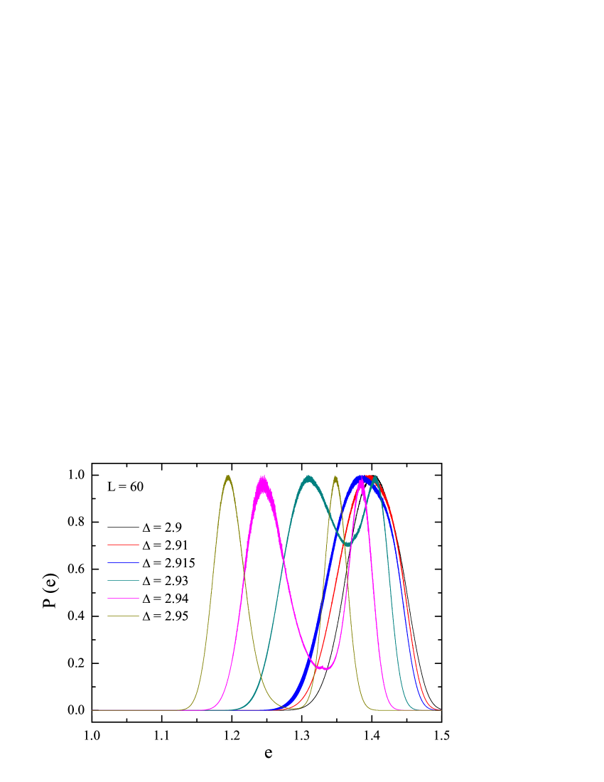
Figure 1: Energy probability density functions for a lattice size $L=60$ and several values of the crystal field, as indicated. For the cases of a double-peaked structure we have used the temperature where the two peaks are of equal height, whereas in the other single-peaked cases, we plot the densities at the corresponding pseudocritical temperatures of the specific heat.

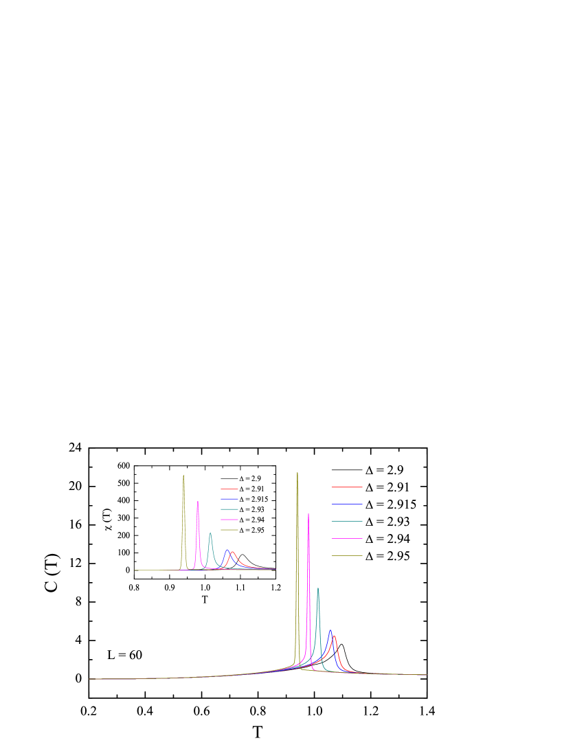
Figure 2: Corresponding specific heats (main panel) and magnetic susceptibilities (inset) as a function of temperature. This figure is complementary to figure 1.

3.1 Second-order phase transition regime

The triangular Blume-Capel model at the crystal field value $\Delta<\Delta_{t}$, undergoes a second-order transition between the ferromagnetic and paramagnetic phases, expected to be in the universality class of the simple $d=2$ Ising model. In the following, we present the finite-size scaling analysis of our numerical data for this case, to verify this expectation. In figure 3 we give an example, for the case $\Delta=1$, of the shift behavior of the pseudocritical temperatures corresponding to the peaks of the following six quantities: specific heat $C$, magnetic susceptibility $\chi$, derivative of the absolute order parameter with respect to the inverse temperature $K=1/T$ ferrenberg91

$$\frac{\partial\langle|M|\rangle}{\partial K}=\langle|M|H\rangle-\langle|M|\rangle\langle H\rangle,$$ (2)

and logarithmic derivatives of the first-, second-, and fourth-order powers of the order parameter with respect to the inverse temperature $K=1/T$ ferrenberg91

$$\frac{\partial\ln\langle M^{n}\rangle}{\partial K}=\frac{\langle M^{n}H\rangle}{\langle M^{n}\rangle}-\langle H\rangle.$$ (3)

Fitting our data to the expected power-law behavior

$$T_{L}^{\ast}=T_{c}+bL^{-1/\nu},$$ (4)

we find the critical temperature to be $T_{c}=2.395(2)$ and the correlation length exponent $\nu=1.007(19)$, in agreement with the value of $\nu=1$ of the simple Ising model. The analysis presented in figure 3 has been performed for all the values of the crystal field considered in the present paper to estimate transition temperatures, but are not shown here for brevity. These values will be used in the sequel in the construction of the phase diagram of the model.

Figure 4 gives an alternative estimation of the correlation length exponent via the finite-size scaling behavior of the logarithmic derivatives of the order parameter, whose maxima are expected to scale (in a second-order phase transition) as $\sim L^{1/\nu}$ with the system size ferrenberg91 . We chose to show in figure 4 the case $n=2$ of equation (3). A simultaneous fitting for all the values of the crystal field considered gives an excellent estimate of $1.008(11)$ for the critical exponent $\nu$ of the correlation length.

We proceed with figures 5 and 6 to estimate the magnetic exponent ratios of the triangular Blume-Capel model. In particular in figure 5 we present the order-parameter data at the estimated critical temperatures as a function of the lattice size. The lines show a simultaneous fitting for the whole spectrum of $\Delta$-values of the form $M_{c}\sim L^{-\beta/\nu}$ that gives an estimate $0.126(2)$ for the critical exponent ratio $\beta/\nu$, in very good agreement with expected value $0.125$ of the pure Ising case. Respectively, in figure 6 we plot the maxima of the magnetic susceptibility, again as a function of the lattice size. As in figure 5, the lines show a simultaneous power-law fitting of the form $\chi^{\ast}\sim L^{\gamma/\nu}$ that gives an estimate $1.756(9)$ for the magnetic exponent ratio $\gamma/\nu$, also in very good agreement with expected value $1.75$ of the pure Ising case.

Closing this subsection, we deal with the most intriguing thermodynamic quantity in the study of spin models: the specific heat. The specific heat is an extremely sensitive quantity and it is well known that it is, at least in some cases, a very hard task to identify with good accuracy its scaling behavior. However, in the present work, our careful numerical implementation of the Wang-Landau scheme and the repeated sampling gave very well numerical data, as can be shown in figure 7, where we present the finite-size scaling behavior of the specific heat maxima. The solid lines show a excellent simultaneous logarithmic fitting of the form

$$C^{\ast}=C_{1}+C_{2}\ln L.$$ (5)

Note here that, the expected logarithmic divergence of the specific heat is very well obtained even from the smaller lattice sizes shown.

Summarizing, the results and analysis presented in this subsection for the triangular Blume-Capel model at its second-order phase transition regime are in full agreement with universality arguments that place the Blume-Capel model for $\Delta<\Delta_{t}$ in the Ising universality class.

Figure 3: Simultaneous fitting of the form (4) of the six pseudocritical temperatures defined in the text for the case $\Delta=1$.

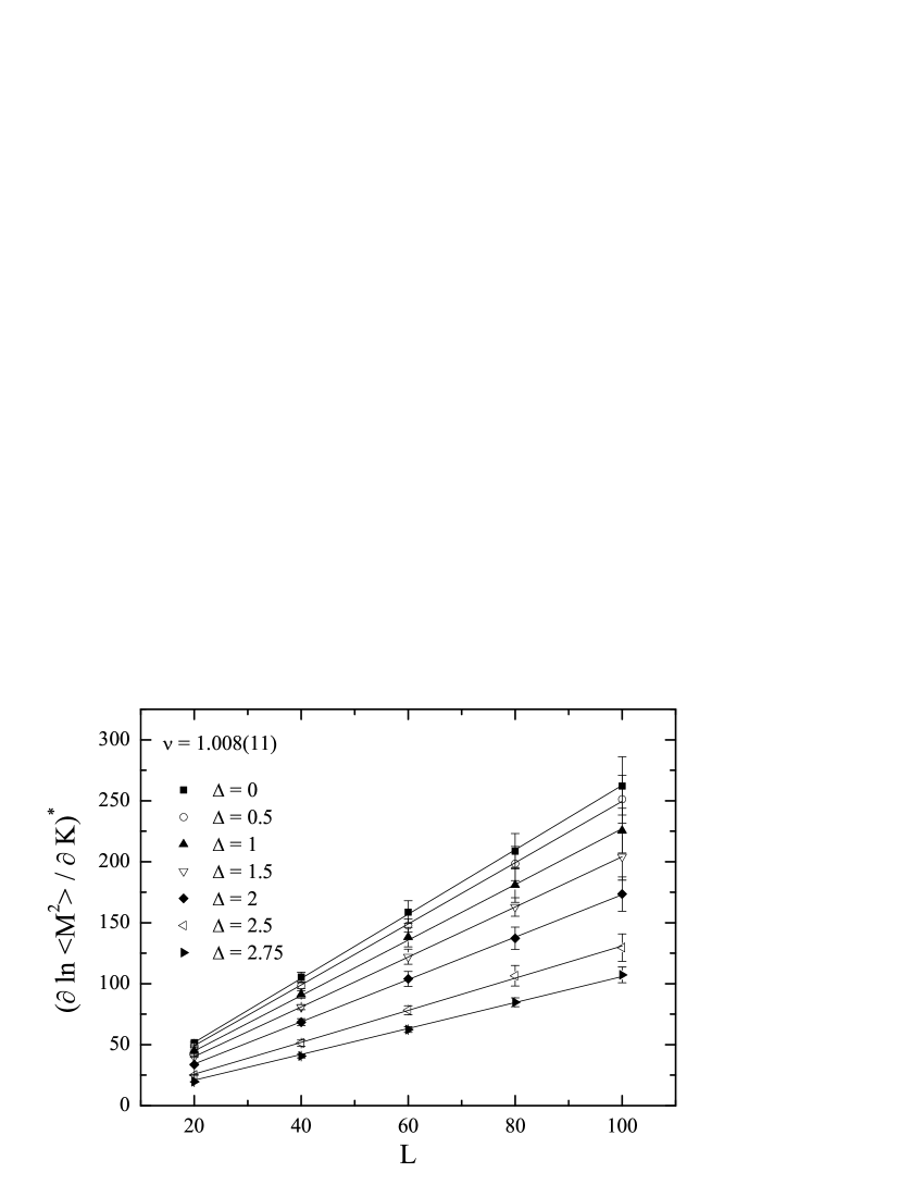
Figure 4: Simultaneous fitting of the maxima of the second-order logarithmic derivative of the order parameter for $\Delta\in[0-2.75]$.

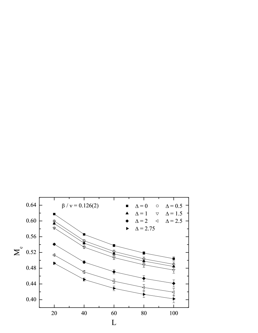
Figure 5: Simultaneous fitting of the critical order-parameter data for $\Delta\in[0-2.75]$.

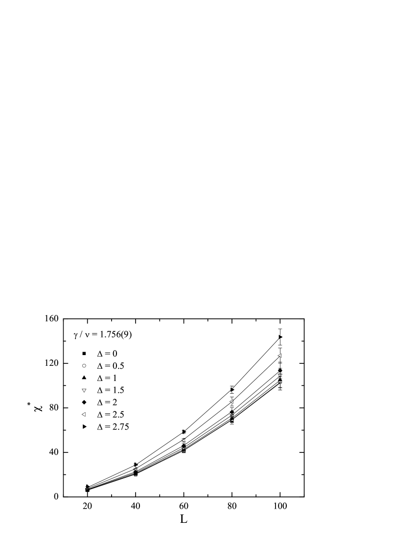
Figure 6: Simultaneous fitting of the maxima of the magnetic susceptibility for $\Delta\in[0-2.75]$.

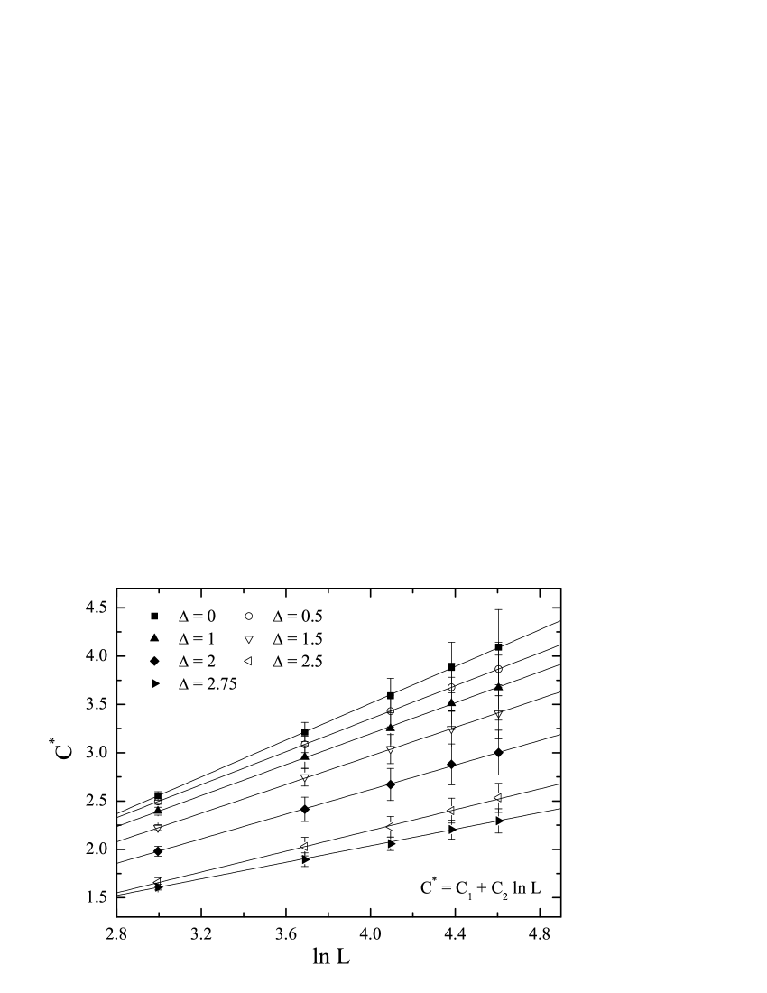
Figure 7: Finite-size scaling of the specific heat maxima. The lines show a simultaneous fitting of the form (5) for $\Delta\in[0-2.75]$. Note the logarithmic scale in the horizontal axis.

3.2 First-order phase transition regime

We now consider the case $\Delta=2.95$, for which the model undergoes a first-order transition between the ferromagnetic and paramagnetic phases. Our first attempt to elucidate the first-order transition features of the present model will closely follow previous analogous studies carried out on the $q\geq 5$ Potts model challa86 ; lee90 ; borgs92 ; janke93 and also our studies of the corresponding square lattice Blume-Capel model malakis and the triangular Ising model with nearest- and next-nearest-neighbor antiferromagnetic interactions malakis07 . As it is well known from the existing theories of first-order transitions, all finite-size contributions enter in the scaling equations in powers of the system size $L^{d}$ fisher82 . This holds for the general shift behavior and also for the finite-size scaling behavior of the peaks of various energy cumulants and of the magnetic susceptibility. It is also well known, as mentioned above, that the double-peaked structure of the energy probability density function $P(e)$ is signaling the emergence of the expected two delta-peak behavior in the thermodynamic limit, for a genuine first-order phase transition binder84 ; binder87 , and with increasing lattice size the barrier between the two peaks should steadily increase. According to the arguments of Lee and Kosterlitz lee90 the quantity $\Delta F(L)/L^{d-1}=[k_{B}T\ln{(P_{max}/P_{min})}]/L$, where $P_{max}$ and $P_{min}$ are the maximum and minimum energy probability density function values at the temperature $T_{h}$ where the two peaks are of equal height, should tend to a non-zero value.

Figure 8: The double-peaked structure of the energy probability density function at $T=T_{h}$ for $\Delta=2.95$ and $L=60$.

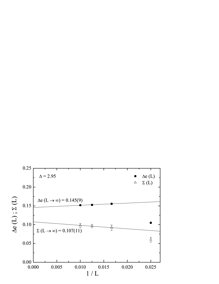
Figure 9: Limiting behavior for $\Delta=2.95$ of the surface tension $\Sigma(L)$, defined in the text, and the latent heat $\Delta e(L)$, shown in figure 8. The solid lines are linear fittings to $L\rightarrow\infty$.

Figure 8 shows the pronounced double-peaked structure of the energy probability density function of the model at the temperature $T=T_{h}$ where the two peaks are of equal height for $L=60$. From the double-peaked energy probability density function one can estimate the surface tension $\Sigma(L)=\Delta F(L)/L$ and the latent heat $\Delta e(L)$, whose values remain finite for a genuine first-order transition. Figure 9 shows the limiting behavior of these two quantities and verifies the persistence of the first-order character of the transition at $\Delta=2.95$. The limiting values of $\Sigma(L)$ and $\Delta e(L)$ are given in the graph by extrapolating at the larger lattice sizes studied.

Figures 10 and 11 illustrate that the traditionally used divergences in finite-size scaling of the specific heat $C$ and susceptibility $\chi$ follow very well a power-law behavior of the form $\sim L^{d}$, as expected for first-order transitions binder84 ; binder87 . Furthermore, figure 12 demonstrates that the divergences corresponding to the first-, second-, and fourth-order logarithmic derivatives of the order parameter defined in equation (3) follow also very well the same $L^{d}$ behavior, as expected.

Figure 10: Finite-size scaling behavior of the specific heat peaks at $\Delta=2.95$ giving a clear $L^{d}$ divergence.

Figure 11: Finite-size scaling behavior of the susceptibility maxima at $\Delta=2.95$. A clear $L^{d}$ divergence is observed as in the case of the specific heat.

Figure 12: Simultaneous fitting of the maxima of the three logarithmic derivatives of the order parameter (3) for $n=1$, $2$, and $4$, at $\Delta=2.95$. As in figures 10 and 11 a clear $L^{d}$ divergence is observed.

In this subsection we have presented a reliable analysis of the first-order transition features of the triangular Blume-Capel model at the value $\Delta=2.95$ of the crystal field and we have verified all the theoretical expectations of finite-size scaling in first-order phase transitions. Additionally, we have estimated important features of this transition, i.e. the surface tension and latent heat of the transition, using the well-established method of Lee and Kosterlitz lee90 .

3.3 Phase diagram and tricriticality

We close this Section with our results on the phase diagram of the model and the related issue of tricriticality. From figure 7 of subsection 3.1 one can observe the expected Ising logarithmic divergence of the specific-heat maxima. Avoiding the value $\Delta=0$, which suffers from (small) crossover effects, we attempted to estimate the tricritical value of the crystal field by fitting the decreasing logarithmic amplitudes $C_{2}$ estimated in the simultaneous fitting of figure 7 to a suitable power law, as shown in the figure 13. This may look like a questionable idea, since the behavior of specific heat data is the Achilles’ heel of finite-size scaling analysis. Yet, figure 13 shows that besides the rather large errors in the logarithmic amplitudes $C_{2}$, one may approximately estimate the tricritical crystal-field value to be $\Delta_{t}=2.925(8)$, as shown in the panel of the figure, in excellent agreement with the previous analysis of the energy probability density functions and the related thermodynamic quantities of figures 1 and 2. We should note here that, such an idea was first suggested and performed in the recent papers of reference malakis for the cases of the pure and random-bond square Blume-Capel model, where it has also produced quite acceptable results. Furthermore, we aim here only to a qualitative prediction of the tricritical crystal field value. A most accurate prediction of these first-order transition features of the phase diagram of the model should follow different routes, well-established in the literature, which are, in any case, well beyond the scope of the present paper.

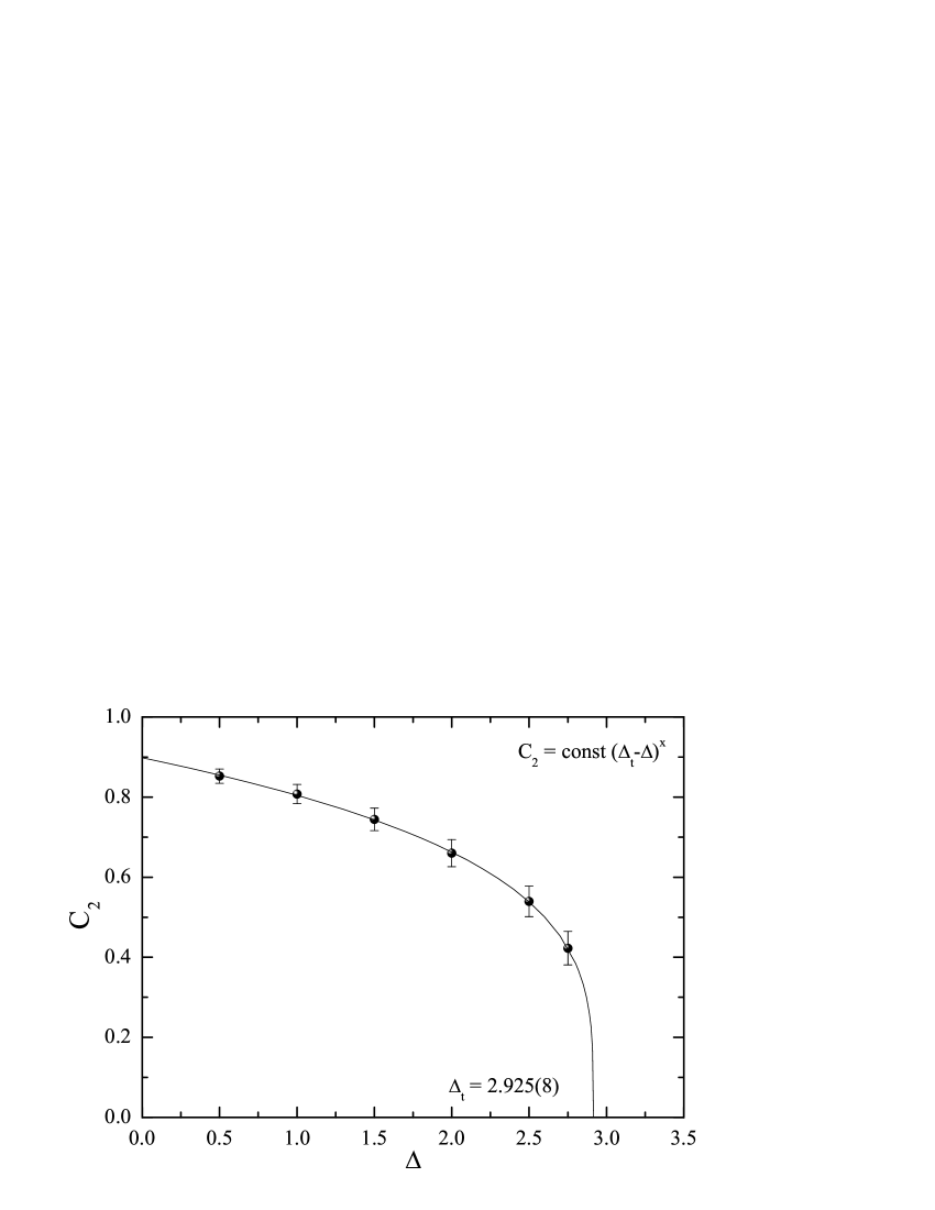
Figure 13: An approximate estimation of the tricritical value of the crystal field by fitting the decreasing logarithmic amplitudes $C_{2}$ of the model [see equation (5)] at suitable values of the crystal field to a power law, as shown in the figure.

Using now our estimates for the transition temperatures obtained throughout this paper for all the values of the crystal field considered we attempt to construct in figure 14 an approximation of the phase diagram of the model. We have fitted the points shown in figure 14 using the following power-law ansatz

$$T\sim(\Delta_{0}-\Delta)^{x},$$ (6)

where $\Delta_{0}$ in the above equation (6) denotes the crossing of the boundary to the horizontal axis ($T=0$) and should take the value $3(=zJ/2)$ for the present case of the triangular lattice ($z=6$). The solid and dotted curves that correspond to second- and first-order phase transitions lines that separate the ordered from the paramagnetic phase have been obtained from a fitting of the form (6) that gives the value $3.01(2)$ for $\Delta_{0}$, very close to the expected value, and a value $x=0.274(9)$ for the exponent. Using now equation (6) and the estimate for the $\Delta_{t}$ from figure 13 we obtain an estimate for $T_{t}=1.025(10)$. Thus, the overall estimate for the tricritical point is $(\Delta_{t},T_{t})=(1.025(10),2.925(8))$ and is marked with a black rhombus in figure 14. We should note here that, although with the power-law fitting (6) we get a very nice estimate for the value $\Delta_{0}$ and also an excellent concurrence between numerically estimated transition points and the applied law, our attempt above aims only at a numerical quantitative approximation for the main part of the diagram and not at the correct asymptotic behavior at its ends. In fact, is well known that the asymptotic approach of phase boundaries to the sections with the axis follows specific power-law behaviors with exponents related to the critical exponents describing the transitions in these part of the diagram aharony .

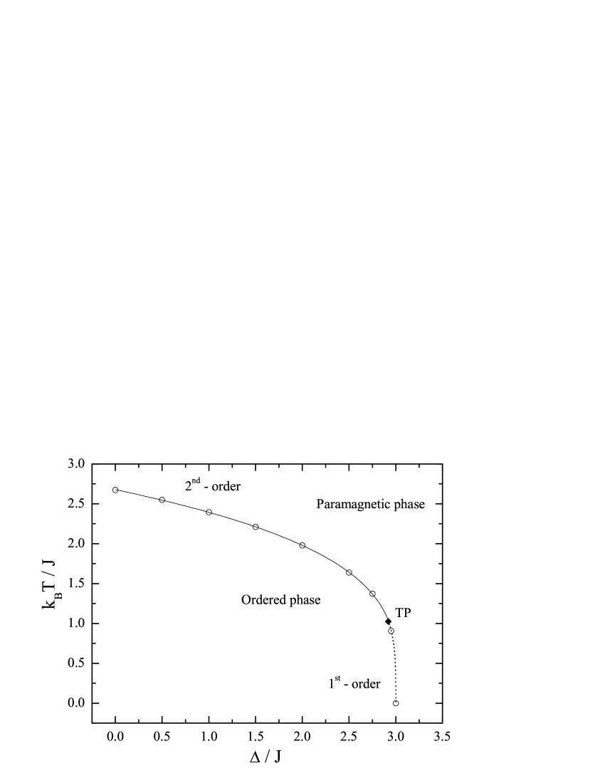
Figure 14: Approximation of the phase diagram of the triangular Blume-Capel model. The dotted and solid curves correspond respectively to first- and second-order phase transition lines that separate the ordered and paramagnetic phases. The black rhombus points the approximate location of the tricritical point (TP).

4 Conclusions

In the present paper we have performed a careful numerical investigation of the critical properties of the Blume-Capel model embedded in the triangular lattice. By applying an extensive two-stage Wang-Landau entropic sampling we have studied the finite-size scaling properties of the model for several values of the crystal field in both its first- and second-order phase transition regime and we have estimated with high accuracy transition temperatures and critical exponents.

In particular, for the regime of second-order phase transitions we have verified the theoretical expectation that the Blume-Capel model belongs to the universality class of the simple $d=2$ Ising model, whereas for the regime of first-order phase transitions we have identified the most characteristic features signaling a first-order phase transition and we have estimated the surface tension and latent heat of the transition using the method of Lee and Kosterlitz. Finally, using our estimates for the transition temperatures and a novel scheme that takes advantage of the logarithmic scaling behavior of the specific heat, we have proposed an approximation of the phase diagram of the model in the overall $(\Delta,T)$-plane and we have refined previous mean-field-type estimates for the tricritical point.

Closing, we would like to leave as an open research challenge the investigation of the phase diagram of the triangular Blume-Capel model via a multi-parametric Wang-Landau method that would give direct access to the estimation of the phase diagram. Such an analysis would be complementary to the present contribution and has been already successfully performed by Silva et al. silva for the case of the square lattice Blume-Capel model.

- (1) M. Blume, Phys. Rev. 141, 517 (1966)
- (2) H.W. Capel, Physica (Utr.) 32, 966 (1966); H.W. Capel, Physica (Utr.) 33, 295 (1967); H.W. Capel, Physica (Utr.) 37, 423 (1967)
- (3) I.D. Lawrie, S. Sarbach, in: C. Domb, J.L. Lebowitz (Eds.), Phase Transitions and Critical Phenomena, Vol. 9 (Academic Press, London, 1984)
- (4) W. Selke, J. Oitmaa, J. Phys. C 22, 076004 (2010)
- (5) D.P. Landau, Phys. Rev. Lett. 28, 449 (1972); A.N. Berker, M. Wortis, Phys. Rev. B 14, 4946 (1976); M. Kaufman, R.B. Griffiths, J.M. Yeomans, M. Fisher, Phys. Rev. B 23, 3448 (1981); W. Selke, J. Yeomans, J. Phys. A 16, 2789 (1983); D.P. Landau, R.H. Swendsen, Phys. Rev. B 33, 7700 (1986); J.C. Xavier, F.C. Alcaraz, D. Pena Lara, J.A. Plascak, Phys. Rev. B 57, 11575 (1998)
- (6) M.J. Stephen, J.L. McColey, Phys. Rev. Lett. 44, 89 (1973); T.S. Chang, G.F. Tuthill, H.E. Stanley, Phys. Rev. B 9, 4482 (1974); G.F. Tuthill, J.F. Nicoll, H.E. Stanley, Phys. Rev. B 11, 4579 (1975); F.J. Wegner, Phys. Lett. 54A, 1 (1975)
- (7) P.F. Fox, A.J. Guttmann, J. Phys. C 6, 913 (1973); T.W. Burkhardt, R.H. Swendsen, Phys. Rev. B 13. 3071 (191976); W.J. Camp, J.P. Van Dyke, Phys. Rev. B 11, 2579 (1975)
- (8) P. Nightingale, J. Appl. Phys. 53, 7927 (1982)
- (9) P.D. Beale, Phys. Rev. B 33, 1717 (1986)
- (10) C.J. Silva, A.A. Caparica, J.A. Plascak, Phys. Rev. E 73, 036702 (2006)
- (11) D. Hurt, M. Eitzel, R.T. Scalettar, G.G. Batrouni, in: Computer Simulation Studies in Condensed Matter Physics XVII, Springer Proceedings in Physics, Vol. 105, Eds. D.P. Landau, S.P. Lewis, H.-B. Schüttler, Springer-Verlag, Berin (2007)
- (12) A. Malakis, A.N. Berker, I.A. Hadjiagapiou, N.G. Fytas, Phys. Rev. E 79, 011125 (2009); A. Malakis, A.N. Berker, I.A. Hadjiagapiou, N.G. Fytas, T. Papakonstantinou, Phys. Rev. E 81, 041113 (2010)
- (13) G.D. Mahan, S.M. Girvin, Phys. Rev. B 17, 4411 (1978)
- (14) A. Du, Y.Q. Yü, H.J. Liu, Physica A 320, 387 (2003)
- (15) X.F. Qian, Y. Deng, and H.W.J. Blöte, Phys. Rev. E 72, 056132 (2005)
- (16) F. Wang, D.P. Landau, Phys. Rev. Lett. 86, 2050 (2001); F. Wang, D.P. Landau, Phys. Rev. E 64, 056101 (2001)
- (17) A. Malakis, A. Peratzakis, N.G. Fytas, Phys. Rev. E 70, 066128 (2004); A. Malakis, S.S. Martinos, I.A. Hadjiagapiou, N.G. Fytas, P. Kalozoumis, Phys. Rev. E 72, 066120 (2005)
- (18) A. Malakis, N.G. Fytas, Phys. Rev. E 73, 016109 (2006)
- (19) N.G. Fytas, A. Malakis, and K. Eftaxias, J. Stat. Mech.: Theory Exp. (2008) P03015
- (20) N.G. Fytas, A. Malakis, and I.A. Hadjiagapiou, J. Stat. Mech.: Theory Exp. (2008) P11009
- (21) R.E. Belardinelli, V.D. Pereyra, Phys. Rev. E 75, 046701 (2007)
- (22) K. Binder, D.P. Landau, Phys. Rev. B 30, 1477 (1984)
- (23) K. Binder, Rep. Prog. Phys. 50, 783 (1987)
- (24) A.M. Ferrenberg, D.P. Landau, Phys. Rev. B 44, 5081 (1991)
- (25) M.S.S. Challa, D.P. Landau, K. Binder, Phys. Rev. B 34, 1841 (1986)
- (26) J. Lee, J.M. Kosterlitz, Phys. Rev. Lett. 65, 137 (1990); J. Lee, J.M. Kosterlitz, Phys. Rev. B 43, 3265 (1991)
- (27) C. Borgs, W. Janke, Phys. Rev. Lett. 68, 1738 (1992)
- (28) W. Janke, Phys. Rev. B 47, 14757 (1993)
- (29) A. Malakis, N.G. Fytas, P. Kalozoumis, Physica A 383, 351 (2007)
- (30) M.E. Fisher, A.N. Berker, Phys. Rev. B 26, 2507 (1982)
- (31) A. Aharony, Phys. Rev. B 18, 3318 (1978); A. Aharony, Phys. Rev. B bf 18, 3328 (1978); T. Schneider, E. Pytte, Phys. Rev. B 15, 1519 (1977); D. Andelman, Phys. Rev. B 27, 3079 (1983); D. Andelman, A.N. Berker, Phys. Rev. B 29, 2630 (1984); Y. Shapir, A. Aharony, J. Phys. C 14, L905 (1984)