Zeno effect and ergodicity in finite-time quantum measurements

Abstract

We demonstrate that an attempt to measure a non-local in time quantity, such as the time average ${\langle}A{\rangle}_{T}$ of a dynamical variable $A$, by separating Feynman paths into ever narrower exclusive classes traps the system in eigensubspaces of the corresponding operator $\hat{A}$. Conversely, in a long measurement of ${\langle}A{\rangle}_{T}$ to a finite accuracy, the system explores its Hilbert space and is driven to a universal steady state in which von Neumann ensemble average of $\hat{A}$ coincides with ${\langle}A{\rangle}_{T}$. Both effects are conveniently analysed in terms of singularities and critical points of the corresponding amplitude distribution and the Zeno-like behaviour is shown to be a consequence of conservation of probability.

Quantum Zeno effect (see, for instance, Z0 -Z2 and Refs. therein) is often associated with the perturbation frequent projective von Neumann measurements vN made on the observed system. Suppose, for example, that one wishes to determine the duration $\tau_{\Omega}$ a quantum system spends in a particular subspace $\Omega$ of its Hilbert space. Checking ever more frequently whether the system is indeed inside $\Omega$ one eventually destroys the transitions between $\Omega$ and the rest of the Hilbert space. Thus, because of the Zeno effect, a continuoulsy observed system prepared inside $\Omega$ would spend there all available time, while for a system initially outside $\Omega$, $\tau_{\Omega}$ would be exactly zero ZW . Alternatively, one can perform a finite time measurement of $\tau_{\Omega}$ in which a meter monitors the system over a finite period of time, and one single observation is made at the end of the run. One example of such a meter is Larmor clock consisting of a spin which rotates only when the system resides in $\Omega$. From the clock’s final orientation one is able to determine the value of $\tau$, but can learn nothing about the precise moments the system enters and leaves $\Omega$. A conceptually similar measurement of the duration $\tau_{q}$ a qubit spends in its state $|q{\rangle}$ proposed in S1 employs a large number of bosons (e.g, a weakly interacting Bose-Einstein condensate) trapped in one of the wells of a symmetric double well potential. With atomic current between the wells increased whenever the qubit occupies the state of interest, the number of bosons found in the other well contains, like a reading of a Larmor clock, information about $\tau(q)$. The purpose of this paper is twofold: we analyse the Zeno effect arising in the high accuracy limit of a general finite-time measurement. We also study the effects of a measurement of long-time average of a quantum variable and search for any evidence of ergodic behaviour. Various approaches to quantum ergodicity can be found in Refs. E1 - E3 , with the importance of measurement(s) performed on the system emphasised in E2 . A variant of the Zeno effect arising solely from strong interaction between a system and its environment has been studied in Z2 .

Consider a quantum system in an $N$-dimensional Hilbert space with a Hamiltonian $\hat{H}$. Choosing an orthogonal basis $|a_{m}{\rangle}$, $m=1,2,..N$ in which $\hat{H}$ is not diagonal, we can write a transition amplitude between initial and final states $|i{\rangle}$ and $|f{\rangle}$ over a time $T$ as a sum over Feynman paths

$$U^{f\leftarrow i}(T)\equiv{\langle}f|\exp(-i\hat{H}T|i{\rangle}=lim_{K\rightarrow\infty}\sum_{m_{1},..,m_{K}}^{N}{\langle}f|a_{m_{K}}{\rangle}\times$$

$$\prod_{j=1}^{K-1}{\langle}a_{m_{j+1}}|\exp(-i\hat{H}\epsilon|a_{m_{j}}{\rangle}{\langle}a_{m_{1}}|i{\rangle}\equiv\sum_{paths}U^{f\leftarrow i}[path],\quad\quad$$ (1)

where $\epsilon\equiv T/(K-1)$ and each path is defined by a sequence $\{m_{1},...,m_{K}\}$ numbering the states $|a_{m}{\rangle}$ through which the system passes until reaching the final state $|f{\rangle}$. Consider a quantity $A$ represented by an operator $\hat{A}$ diagonal in the chosen representation,

$$\hat{A}=\sum_{n}A_{n}\hat{P}_{n},\quad\hat{P}_{n}\hat{P}_{m}=\hat{P}_{n}\delta_{mn},\quad\sum_{n}\hat{P}_{n}=1,$$ (2)

where $\hat{P}_{n}$ are mutually orthogonal projectors on (one- or multidimensional) subspaces spanned by vectors $|a_{m}{\rangle}$ corresponding to the same eigenvalue $A_{n}$. We wish to measure the value of a Feynman functional

$$F[path]=lim_{K\rightarrow\infty}\sum_{j=1}^{K-1}\beta(j\epsilon)A_{m_{j}}\epsilon$$ (3)

$$\equiv\int_{0}^{T}\beta(t)A(t)dt$$

where $\beta(t)$ is a known function FOOT1 and $A(t)$ denotes the (highly irregular) function traced by the value of $A$ along a given Feynman path. Equation (3) may, for example, represent the time average of a quantity $A$ if one chooses $\beta(t)=1/T=const$ and, in particular, the fraction of the time, $\tau_{\Omega}/T$, the system has spent in $\Omega$ if $\hat{A}$ is also chosen to be the projector onto a subspace $\Omega$ spanned by $|a_{n}{\rangle}$, $\hat{A}=\hat{P}_{\Omega}\equiv\sum_{n\in\Omega}|a_{n}{\rangle}{\langle}a_{n}|$ S1 . The probability amplitude for the value of $F$ to be $y$ is given by the restricted path sum

$$\Phi^{f\leftarrow i}(y,T)=\sum_{paths}\delta(F[path]-y)U^{f\leftarrow i}[path].$$ (4)

where $\delta(z)$ is the Dirac delta. Without loss of generality we choose the measuring device to be a Neumann pointer with position $y$ which interacts with the system over a time $T$, the full Hamiltonian being $\hat{\mathcal{H}}(t)=\hat{H}-i\partial_{y}\beta(t)\hat{A}$. At $t=T$ the pointer states of the meter, $|y{\rangle}$, are entangled with the system’s states obtained by propagation along Feynman paths satisfying the condition $F[path]=y$ S2 . In particular, for the system and the meter prepared at $t=0$ in an product state $|i{\rangle}|G{\rangle}$, the probability amplitude to find at $t=T$ the system in the state $|f{\rangle}$ and, simultaneously, the pointer reading $y$, $\Psi^{f\leftarrow i}(y)$, is given by

$$\Psi^{f\leftarrow i}(y,T)\equiv{\langle}y|{\langle}f|\exp[-i\int_{0}^{T}\hat{\mathcal{H}}(t)dt]|i{\rangle}|G{\rangle}=$$

$$\int G(y-y^{\prime})\Phi^{f\leftarrow i}(y^{\prime},T)dy,$$ (5)

where $G(y)\equiv{\langle}y|G{\rangle}$. Note that the second of Eqs.(Zeno effect and ergodicity in finite-time quantum measurements) is not specific to our choice of von Neumann meter and occurs for a wider class of quantum measurements, e.g., for the one considered in S1 . With $G(y)$ narrowly peaked around the origin, Feynman paths with different values of $F[path]$ contribute to different final meter states, and $|\Psi^{f\leftarrow i}(y)|^{2}$ yields the probability to reach the final state and obtain the value $y$ for the quantity in Eq.(3). The measured result contains, however, an intrinsic quantum uncertainty as the values of $y^{\prime}$ within the peak’s width around $y$ remain indistinguishable. With many different Feynman paths contributing to the transition (Zeno effect and ergodicity in finite-time quantum measurements) one might expect the values of $F$ to have a broad distribution, which a more accurate measurement would resolve in ever greater detail. The accuracy can be improved by making the initial pointer state narrower in the coordinate space, e.g., by replacing $G(y)$ with

$$G_{\alpha}(y)=\alpha^{1/2}G(\alpha y),\quad\quad lim_{\alpha\rightarrow\infty}|G_{\alpha}(y)|^{2}=\delta(y)$$ (6)

where the factor $\alpha^{1/2}$ ensures the correct normalisation of the new state, $\int|G_{\alpha}(y)|^{2}dy=\int|G(y)|^{2}dy=1$ .

With the help of Eqs.(Zeno effect and ergodicity in finite-time quantum measurements) and (6) we can now prove a general result: an accurate finite time measurement, $\alpha\rightarrow\infty$, $T<\infty$, would indicate that at all times $A(t)$ maintains a constant value equal to one of the eigenvalues $A_{n}$, with the value of the functional (3) equal exactly to $A_{n}\int_{0}^{T}\beta(t)dt$. The proof follows from observing first that $\Phi^{f\leftarrow i}(y)$ cannot be a smooth function for all final states $|f{\rangle}$. Indeed, increasing $\alpha$ while maintaining unit normalisation will cause the integral $\int G_{\alpha}(y)dy=\alpha^{-1/2}\int G(y)dy$ to vanish. With it would also vanish $\Psi^{f\leftarrow i}(y)$, $\lim_{\alpha\rightarrow\infty}\Psi^{f\leftarrow i}(y)=\Phi^{f\leftarrow i}(y)\alpha^{-1/2}\int G(y-y^{\prime})dy^{\prime}=0$, thus contradicting conservation of probability for the pointer. Thus, $\Phi^{f\leftarrow i}(y)$ must have a singular part, which we evaluate by rewriting Eq.(4) as a Fourier integral

$$\Phi^{f\leftarrow i}(y)=\quad\quad\quad$$ (7)

$$(2\pi)^{-1}\int\exp(i\lambda y){\langle}f|\exp[-i\int_{0}^{T}(\hat{H}+\lambda\beta(t)\hat{A})dt]|i{\rangle}d\lambda.$$

Further, writing $\exp\{-i\int_{0}^{T}[\hat{H}+\lambda\beta(t)\hat{A}]dt\}=lim_{K\rightarrow\infty}\prod_{j=1}^{K}\exp\{-i[\hat{H}+\lambda\beta(jT/K)\hat{A}]T/K\}$ we note that $lim_{\lambda\rightarrow\infty}\exp\{-i[\hat{H}+\lambda\beta(jT/K)\hat{A}]T/K\}=\sum_{n}\exp\{-i\lambda\beta(jT/K)A_{n}\}\exp(-i\hat{P}_{n}\hat{H}\hat{P}_{n}T/K)\hat{P}_{n}+O(\lambda^{-1})$. Defining a Zeno hamiltonian as (c.f. Z2 )

$$\hat{H}_{Z}=\sum_{n}\hat{P}_{n}\hat{H}\hat{P}_{n},$$ (8)

we obtain

$${\langle}f|\exp[-i\int_{0}^{T}(\hat{H}+\lambda\beta(t)\hat{A})dt]|i{\rangle}=\quad\quad\quad$$ (9)

$$\sum_{n}\exp\{-i\lambda A_{n}\int_{0}^{T}\beta(t)dt\}{\langle}f|\exp(-i\hat{H}_{Z}T)\hat{P}_{n}|i{\rangle}$$

$$+{\langle}f|\hat{u}(\lambda)|i{\rangle}$$

where the last terms vanishes as $\lambda\rightarrow\pm\infty$, $lim_{\lambda\rightarrow\infty}{\langle}f|\hat{u}(\lambda)|i{\rangle}=O(\lambda^{-1})$. Inserting Eq.(9) into Eq.(7) yields

$$\Phi^{f\leftarrow i}(y)=\sum_{n}{\langle}f|\exp(-i\hat{H}_{Z}T)\hat{P}_{n}|i{\rangle}\times$$ (10)

$$\delta(y-A_{n}\int_{0}^{T}\beta(t)dt)+\Phi^{f\leftarrow i}_{smooth}(y).$$

where $\Phi^{f\leftarrow i}_{smooth}(y)$ is the smooth Fourier transform of the last term in Eq.(9). With the contributions from the smooth term vanishing in the limit $\alpha\rightarrow\infty$ FOOT0 the monitored system is seen to undergo unitary evolution with a reduced Hamiltonian $\hat{P}_{n}\hat{H}\hat{P}_{n}$ in the subspaces corresponding to each of the distinct eigenvalues $A_{n}$, $n=1,2..$. As in the case of the Zeno effect caused by frequent observations,Z0 -Z2 , an accurate finite-time measurement suppresses transitions between different subspaces. Taking trace over the system’s variables we find the probability distribution for the functional (3)

$$lim_{\alpha\rightarrow\infty}W^{i}(y,T)\equiv\sum_{f}|\Phi^{f\leftarrow i}(y,T)|^{2}\approx$$

$$\sum_{n}\delta(y-A_{n}\int_{0}^{T}\beta(t)dt){\langle}i|\hat{P}_{n}|i{\rangle}.$$ (11)

In particular, a strongly observed system starting in a a state corresponding to a non-degenerate eigenvalue, $|i{\rangle}=|a_{M}{\rangle}$, $\hat{P}_{M}=|a_{M}{\rangle}{\langle}a_{M}|$, would follow a constant Feynman path $A(t)=A_{M}$, thus having the time average of $\hat{A}$ exactly equal to $A_{M}$, and spending all available time in its initial state, $\tau_{M}=T$. This failure to find real evidence of the irregular virtual motion suggested in Eq.(Zeno effect and ergodicity in finite-time quantum measurements) by separating Feynman paths into ever narrower exclusive classes according to the value of a functional (3) constitutes the finite-time Zeno effect and is the first result of this paper.

Next we show that the evidence of the virtual motion is recovered if one performes a long measurement of an arbitrarily high but fixed accuracy, $\alpha<\infty$ and $T\rightarrow\infty$. For simplicity we consider the time average of $A$, thus choosing $\beta(t)=1/T=const$. Changing variables in Eq.(7), $z=\lambda/T$, and using spectral representation for the operator $\hat{H}+z\hat{A}$ yields

$$\Phi^{f\leftarrow i}(y)=(2\pi)^{-1}T\times\quad\quad\quad$$ (12)

$$\sum_{n=1}^{N}\int{\langle}f|\psi_{n}(z){\rangle}\exp\{i[zy-\mathcal{E}_{n}(z)]T\}{\langle}\psi_{n}(z)|i{\rangle}dz.$$

where $(\hat{H}+z\hat{A})|\psi_{n}(z){\rangle}=\mathcal{E}_{n}(z)|\psi_{n}(z){\rangle}$. The long time behaviour of $\Phi^{f\leftarrow i}(y)$ is now determined by the critical points $z_{n}^{s}(y)$ of the exponent in Eq.(12),

$$\partial_{z}\mathcal{E}_{n}(z)_{z=z_{n}^{s}}=y.$$ (13)

Evaluating the integrals in Eq.(12) by the stationary phase method yields $N$ rapidly oscillating contributions containing factors $\exp[iS_{n}(y)T]$ with the phases given by the Legendre transforms of $\mathcal{E}_{n}(z)$, $S_{n}(y)=z_{n}^{s}y-\mathcal{E}_{n}(z_{n}^{s})$. The critical points $y_{n}^{s}$ of $S_{n}(y)$ are determined by the condition $z_{n}^{s}(y_{n}^{s})=0$ so that from Eq.(13) we have $y_{n}^{s}=\partial_{z}\mathcal{E}_{n}(z)|_{z=0}$. Calculating the derivatives with the help of the perturbation theory and evaluating the integrals in Eq.(Zeno effect and ergodicity in finite-time quantum measurements) by the stationary phase method, we find

$$lim_{T\rightarrow\infty}\Psi^{f\leftarrow i}(y)=\quad\quad$$

$$\sum_{n}G_{\alpha}(y-{\langle}\phi_{n}|A|\phi_{n}{\rangle}){\langle}f|\phi_{n}{\rangle}\exp(-iE_{n}T){\langle}\phi_{n}|i{\rangle},$$ (14)

where $\hat{H}|\phi_{n}{\rangle}=E_{n}|\phi_{n}{\rangle}$. Extension to mixed states is straightforward. For an initial state $\hat{\rho}_{i}$, all $E_{n}$ non-degenerate and all ${\langle}\phi_{n}|A|\phi_{n}{\rangle}$ distinct, the probability distribution of the meter’s readings is given by

$$lim_{\alpha\rightarrow\infty}lim_{T\rightarrow\infty}W^{i}(y,T)=$$ (15)

$$\sum_{n}\delta(y-{\langle}\phi_{n}|\hat{A}|\phi_{n}{\rangle}){\langle}\phi_{n}|\hat{\rho}_{i}|\phi_{n}{\rangle},$$

where the order in which the limits are taken is essential.

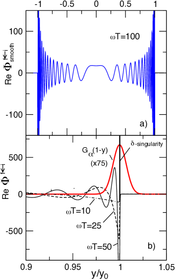
Figure 1: (colour online) a) Amplitude distribution $\Phi^{f\leftarrow i}_{smooth}(y,T)$ for $|i{\rangle}=|1{\rangle}$, $|f{\rangle}=|+{\rangle}$, $\hat{H}=\omega\hat{\sigma}_{z}$, $\hat{A}=\hat{\sigma}_{y}$, and $\omega T=100$; b) $\Phi^{f\leftarrow i}_{smooth}(y,T)$ for $\omega T=50$ (solid), $\omega T=25$ (dashed), and $\omega T=10$ (dot-dashed). Also shown is $G_{\alpha}(1-y)$ ($\times 75$) for $\alpha=100$ (thick solid).

We note that a strongly observed system prepared with a known energy $E_{k}$, ${\langle}\phi_{n}|\hat{\rho}_{i}|\phi_{n}{\rangle}=\delta_{kn}$, explores its Hilbert space is such a way that the long-time time average of a dynamical variable $A$ is sharply defined, with the value equal to the ensemble average in the projection von Neumann measurement of the operator $\hat{A}$, ${\langle}\phi_{k}|\hat{A}|\phi_{k}{\rangle}$. In particular, as $T\rightarrow\infty$, the fraction of time a system prepared in a pure state $|\phi_{k}{\rangle}$ spends in a subspace $\Omega$ spanned by the subset of eigenvectors {$|a_{m}{\rangle},m\in\Omega\}$ tends to the measure of the subset $\mu_{\Omega}=\sum_{m\in\Omega}|{\langle}a_{m}|\phi_{k}{\rangle}|^{2}$ This ergodic-like FOOTN property of bound quantum motion, to our knowledge not yet discussed in literature, is the second result of this paper. Further, as seen from Eq.(Zeno effect and ergodicity in finite-time quantum measurements), a system starting in a mixed state $\hat{\rho}_{i}$, undergoes relaxation to the same steady state diagonal in the energy representation, $\hat{\rho}_{f}=\sum_{n}|\phi_{n}{\rangle}{\langle}\phi_{n}|\hat{\rho}_{i}|\phi_{n}{\rangle}{\langle}\phi_{n}|$, regardless of the choice of $\hat{A}$. Thus, finite-time average of a quantity $A$, ${\langle}A{\rangle}_{T}\equiv\int yW^{i}(y,T)dy$, tends, as $T\rightarrow\infty$, to the von Neumann ensemble average $Tr\{\hat{A}\hat{\rho}_{f}\}$. As in the case of a frequently observed system E3 the equivalence between the time- and ensemble averages is established in the state produced at the end of measurement, $\hat{\rho}_{f}$, rather that in the initial state $\hat{\rho}_{i}$.

We illustrate the above with a simple example, where one wishes to measure the time average of the $y$-component of a spin $1/2$, $\hat{A}\equiv\hat{\sigma}_{y}$, for a two-level system with Hamiltonian $\hat{H}=\omega\hat{\sigma}_{x}$ prepared in its eigenstate $|1{\rangle}$, $\hat{H}|1,2{\rangle}=\pm\omega|1,2{\rangle}$. Choosing in Eq.(3) $\beta=const$ we then convert to dimensionless variables, $T\rightarrow\omega T$, $y\rightarrow y/y_{0}$, $y_{0}\equiv\beta T$, $\beta\rightarrow 1/T$. As in Ref.S1 , $G(y)$ in Eq.(Zeno effect and ergodicity in finite-time quantum measurements) is chosen to be a Gaussian,

$$G_{\alpha}(y)=(2/\pi)^{1/4}(\alpha)^{1/2}\exp(-\alpha^{2}y^{2}).$$ (16)

Figure 1a shows $\Phi^{+\leftarrow 1}_{smooth}(y)$, $\hat{\sigma}_{z}|\pm{\rangle}=\pm|\pm{\rangle}$, for $\omega T=100$, with the stationary region clearly seen around $y_{2}^{s}=y_{1}^{s}={\langle}1|\hat{\sigma}_{y}|1{\rangle}=0$.

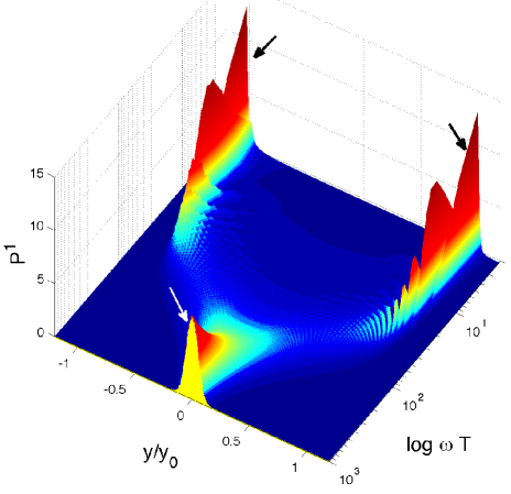
Figure 2: (colour online) Probability distribution of the time average of the $y$-component of the spin, $\hat{A}=\hat{\sigma}_{y}$, for a two-level system with the Hamiltonian $\hat{H}=\omega\hat{\sigma}_{x}$ vs. the averaging time $T$. The system is prepared in the eigenstate $|1{\rangle}$, $\hat{H}|1{\rangle}=\omega|1{\rangle}$, and the accuracy of the measurement is $\Delta y/y_{0}=0.05$. The ergodic peak and two Zeno peaks are indicated by white and black arrows, respectively.

Two Zeno peaks at $y/y_{0}=\pm 1$ predicted by Eq.(Zeno effect and ergodicity in finite-time quantum measurements) and a single ’ergodic’ (for want of a better word) peak predicted by Eq.(15) are shown in Fig.2. Transition between the regimes described by Eqs.(Zeno effect and ergodicity in finite-time quantum measurements) and (15) occurs as the Zeno peaks, however narrow $G_{\alpha}$ may be, are eventually cancelled by the contributions from $\Phi^{f\leftarrow i}_{smooth}(y)$, whose oscillations become more rapid as the time $T$ increases. This is illustrated in Fig. 1b, for the spin-$1/2$ system described above, with $\Psi^{+\leftarrow 1}(y=1)$ given by Eq.(Zeno effect and ergodicity in finite-time quantum measurements). For $\omega T=10$ the contribution from $\Phi^{+\leftarrow 1}_{smooth}(y)$ (dot-dashed) is negligible, and the Zeno peak is formed by the $\delta$-singularity of $\Phi^{+\leftarrow 1}$ (c.f. Eq. (10)) at $y=1$. For $\omega T=50$ the contribution of the singular term is largely cancelled by the first negative oscillation of $\Phi^{+\leftarrow 1}_{smooth}(y)$ (solid) that fits under the Gaussian $G_{\alpha}(1-y)$ (thick solid), thus making $\Psi^{+\leftarrow 1}(y=1)$ negligible.

In summary, we have considered a general finite-time measurement based on separating Feynman paths into exclusive classes according to the value of a functional such as time average of a dynamical variable $A$, ${\langle}A{\rangle}_{T}$. We have shown that: (i) A highly accurate measurement of a fixed duration traps the measured system in the eigenstates (eigensubspaces) of the corresponding operator $\hat{A}$. (ii) For any quantity $A$, a prolonged measurement of an arbitrary but fixed accuracy destroys coherences in the energy representation, thus leaving the system in a steady state with ${\langle}A{\rangle}_{T}$ equal to the von Neumann projection average of $\hat{A}$. In the special case of a system prepared in a pure stationary state, ${\langle}A{\rangle}_{T}$ is sharply defined, and the proportion of time spent in a given subspace $\Omega$ is exactly equal to the von Neumann probability to find the system there. Both effects are readily explained in terms of singularities and critical points of the corresponding amplitude distribution. Present analysis can be extended to the cases of ’self-measurement’, such as wavepacket tunnelling S3 , where no external meter is employed.

This work was supported by the Basque Goverment grant IT472 and MICINN (Ministerio de Ciencia e Innovaci n) grant FIS2009-12773-C02-01.

References

(1) D.Home and M.A.B. Whitaker, Ann. Phys., 258, 237 (1997).
(2) P.Facchi, H. Nakazato, and S.Pascazio, Phys.Rev.Lett., 86, 2699 (2002)
(3) P.Facchi and S.Pascazio, Phys.Rev.Lett., 89, 080401 (2002)
(4) J. von Neumann, Mathematical Foundation of Quantum Mechanics (Princeton University Press, Princeton, 1955).
(5) For a theory of less restrictive weak continuous measurements see
R.Ruskov, A.N. Korotkov, and A. Mizel, Phys.Rev.B., 73, 085317 (2006)
(6) M. Buettiker, Phys.Rev.B., 27, 6178 (1983);
D.Sokolovski and J.N.L.Connor, Phys.Rev.A, 47, 4677 (1993).
(9) P.Bocchieri and A.Loinger, Phys.Rev., 111, 668 (1958)
(10) M.J.Wilford, J.Phys.A, 19, L1144 (1986)
(11) S. Goldstein, J. L. Lebowitz, C. Mastrodonato, R. Tumulka and N. Zangh
Proc. R. Soc. A 466, 3203 (2010) contains a comprehensive list of relevant references.
(12) We assume in every finite interval of .
(13) D.Sokolovski and R.Sala Mayato, Phys. Rev. A 71, 042101 (2005)
(14)
More precisely, by Parceval’s theorem is a square
integrable function, . Therefore
can have, at most, integrable singularities which
would be even weaker for . Thus the integrals
are finite and would vanish
for .
(15)
We do not address the macroscopic aspect central to most studies of quantum ergodicity
E1 , E2 .
We do, however, address non-trivial statistical behaviour of an
observed completely specified quantum system, something not considered
if an unperturbed Schroedinger evolution is assumed E3 .