Phenomena of complex analytic dynamics in the non-autonomous, nonlinear ring system

Abstract

The model system manifesting phenomena peculiar to complex analytic maps is offered. The system is a non-autonomous ring cavity with nonlinear elements and filters,

Keywords:Mandelbrot and Julia sets; complex analytic maps; ring systems.

¹Kotel’nikov Institute of Radio-Engineering and Electronics of RAS, Saratov Branch
Zelenaya 38, Saratov, 410019, Russian Federation

²Saratov State University
Astrahanskaya 83 Saratov, 410026, Russian Federation

^∗IsaevaO@rambler.ru

When one studies simple quadratic map of a complex variable and with complex parameter

$$z_{n+1}=c+z_{n}^{2}.$$ (1)

the interesting phenomena can be observed. The complex phase plane of a variable $z$, appears subdivided to two domains. The start from one area gives trajectory $z_{n}$, escaping to infinity. The start from another area gives trajectory, remaining restricted: the trajectory wanders not far away from an origin. This second domain is named a Julia set. In a trivial case with $c=0$ it looks as a unit disk. With nonzero parameter values the Julia set is, fractal with non-smouth border, and has self-similar structure (see Fig. 1).

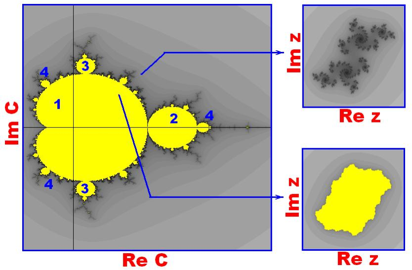
Figure 1: Mandelbrot set (left panel) and Julia sets (right panels) for the complex quadratic map (1) at parameter and phase plane charts. Yellow areas correspond to the periodic dynamics of the complex variable $z$ in a bounded domain (the periods are marked by figures). Black color designates bounded chaotic dynamics. Gray colors correspond to the escape of the trajectories to infinity by different steps of time (more dark color corresponds to more long escape time)

The restricted in a phase space dynamics is possible not with any parameter $c$ values. Moreover, with different parameter values it has different properties – it can be periodic or chaotic. The useful method for examination of a system is the drowing of a chart of a complex parameter plane, for example as a chart of dynamical regimes. At Fig. 1 such chart is represented. On the plane $c$ the object known as a Mandelbrot set is arises. It represents a fractal domain, parameter values from which corresponds to restricted dynamics. Mandelbrot set looks as a cardioid with a set of the attached round lobes (corresponded to periodic dynamics). This ”cartus” is enclosed by fractal ”mane”, corresponded to chaotic dynamics.

The huge amount of the mathematical literature is devoted to Mandelbrot and Julia sets [1-3]. The important task for physicist is the development of physical applications of the theory of complex analytic dynamics and building up of the physical devices and systems in which the complex dynamics is implemented. Just several examples of such systems are exists [4-9]. In the present work a new example of a system in which Mandelbrot set can be implemented is offered. It is a non-autonomous ring system with nonlinear elements and filters. This model can be constructed for example on the basis of an optical system of the Ikeda cavity type [10] or as a ring system with the ferromagnetic structures as nonlinear elements [11].

Let us consider the system represented at Fig. 2. The signal can travel between knots 1-2-3-4. In the optical resonator these are the mirrors, turned around from each other so that a ray of light transits on a ring path. An external pumping C and D exciting the signal in the system are brought at knots 1 and 3. In optical cavity it can be semi-glassy mirrors. Signals C and D have complex slow amplitude $C$ and $D$ and frequency $\omega$.

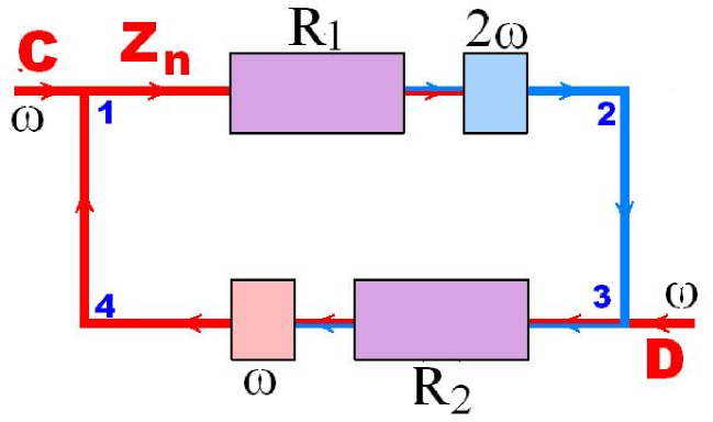
Figure 2: Diagram of the ring device with two nonlinear elements (violet rectangles of length $R_{1}$ and $R_{2}$), two filters, absorbing the signal of frequency $2\omega$ (blue box) and the signal of frequency $\omega$ (pink box). C and D are the external pumping signals of frequency $\omega$. $Z_{n}$ is a complex slow amplitude of the signal (of frequrncy $\omega$) near after the knot, marked as 1

Let us assume that near the knot 1 signal in the ring have slow complex amplitude $Z_{n}$ and frequency $\omega$. By travelimg (the direction is indicated by arrow) a signal spreads through the segment of nonlinear medium of length $R_{1}$, in which the signal transforms. For example the component on doubled frequency. can be excited. Interaction of two these components (in the case of its synchonism and by approximation of statiobarity of waves) can be described by differential equations

$$i\frac{\partial a}{\partial x}=\alpha a^{*}b,\qquad i\frac{\partial b}{\partial x}=\beta a^{2}$$ (2)

where $a(x)$ is a complex slow amplitude of the component on frequency $\omega$, $b(x)$ is a complex slow amplitude of a component on frequency $2\omega$, $x$ is a coordinate along a segment of nonlinear medium. If on an input to a medium the amplitude of component with frequency $\omega$ is $a(0)\sim Z_{n}$, then on an exit in some approximation the amplitude of the component of frequency $2\omega$ is $b(R_{1})\sim Z_{n}^{2}$.

Further a signal runs through a filter which passes only component on frequency $2\omega$. After that the signal is reflected from a knot 2 and a knot 3, where external pumping D of frequency $\omega$ is added. On a segment between the third and fourth knot the nonlinear medium of length $R_{2}$ is located. Transiting through nonlinear medium signal (with a component of frequency $2\omega$ come from the filter and a component of frequency $\omega$ added outside) transforms according to the equations (2). On an exit from a nonlinear medium the component of a signal on frequency $\omega$ in some approximation have intensity $a(R_{2})\leavevmode\nobreak\ D^{*}Z_{n}^{2}$.

Further the signal transits through the filter which passes component on frequency $\omega$. Finally, on a knot 1 there is an additional external pumping C on the same frequency. Complex amplitudes of external signal and signal in the ring accumulates $a(R_{2})+C$. Thus, the signal makes the full circle. It have the same frequency $\omega$ as in the beginning of the path and its complex amplitude can be asymptotically wrote as $Z_{n+1}=F(Z_{n})=C+D^{*}Z_{n}^{2}$. Last expression represents complex map.

Numerical experiment of evolution of a signal in this system is carried out. The equations (2) are integrated (by Runge-Kutta method). As a matter of fact the numerical simulation is divided into some stage: 1) an integration of a system (2) with parameters $\alpha_{1}$, $\beta_{1}$ and with initial conditions $a(0)=Z_{n}$, $b(0)=0$ gives us $a(R_{1})$ and $b(R_{1})$; 2) an integration of a system (2) with parameters $\alpha_{2}$, $\beta_{2}$ and with initial conditions $a(0)=D$, $b(0)=b(R_{1})$ gives us $a(R_{2})$ and $b(R_{2})$; 3) accumulation $a(R_{2})+C$ gives us a new step value of a complex discrete variable $Z_{n+1}$. At Fig. 3 two charts of a plane of parameter $C$ for an investigated system at different values of parameters, characterising the nonlinear media are represented.

Obviously the Poicaré map $Z_{n+1}=F(Z_{n})$ is not complex analytical (it is not satisfies Cauchy–Riemann equations) because system (2) contains non-analytical term, proportional to $a^{*}$. Phenomena of complex analytic dynamics can realise in described model only as a approximation. One can see at Fig. 3 ”almost ideal” Mandelbrot set on top panel which is distorted on bottom panel by the growth of parameters $\alpha_{1}$ and $\beta_{2}$ (leading to amplification of ”non-analyticity”).

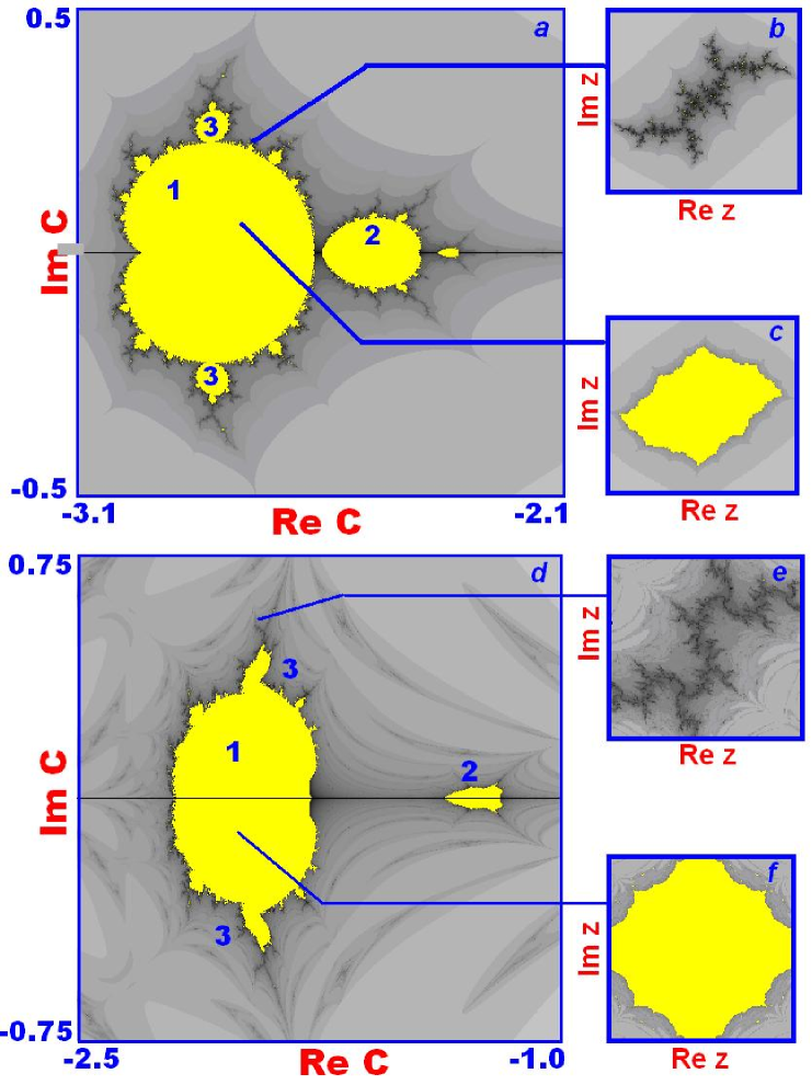
Figure 3: Mandelbrot-like set ($a$, $d$), which arises for the ring cavity represented at Fig. 2, on the chart of the complex plane of a parameter $C$, responsible to the complex slow amplitude of pumping signal C, and Julia-like set ($b$-$c$, $e$-$f$), which arises at he complex plane of the amplitude of the signal $Z$ in the ring in the Poincaré section near knot 1. Values of parameters are: complex slow amplitude of the pumping signal D $D=3$; length of nonlinear elements $R_{1}=R_{2}=1.0$; parameters, characterising media in nonlinear elements $\alpha_{1}=0.01$, $\beta_{1}=1.0$, $\alpha_{2}=1.0$, $\beta_{2}=0.01$ ($a$-$c$) and $\alpha_{1}=0.05$, $\beta_{1}=1.0$, $\alpha_{2}=1.0$, $\beta_{2}=0.1$ ($d$-$f$)

One tool for an analysis of the degree of violation of the complex analyticity, suggested in [12] , is the computation of the spectrum of Lyapunov exponents. In particular, for a two-dimensional map $X_{n+1}=U(X_{n},Y_{n})$, $Y_{n+1}=V(X_{n},Y_{n})$ they may be determined via the eigenvalues of the matrix

$$\mathbf{b}=\mathbf{a}(X_{0},Y_{0})\mathbf{a}^{+}(X_{0},Y_{0})\mathbf{a}(X_{1},Y_{1})\mathbf{a}^{+}(X_{1},Y_{1})...\mathbf{a}(X_{M-1},Y_{M-1})\mathbf{a}^{+}(X_{M-1},Y_{M-1}),$$ (3)

where

$$\mathbf{a}=\left(\begin{array}[]{cc}\partial U(X,Y)/\partial X&\partial U(X,Y)/\partial Y\\ \partial V(X,Y)/\partial X&\partial V(X,Y)/\partial Y\end{array}\right),$$ (4)

In the case of a two-dimensional real map equivalent to an analytic map of one complex variable, two Lyapunov exponents must be equal. It may be shown from the Cauchy-Riemann conditions

$$\begin{array}[]{cc}\partial U(X,Y)/\partial X=\partial V(X,Y)/\partial Y,\\ \partial U(X,Y)/\partial Y=-\partial V(X,Y)/\partial X,\end{array}$$ (5)

that two eigenvalues coincide at any values of parameters and variables. The same is true for the Lyapunov exponents expressed as $\Lambda_{1,2}\sim\log\lambda_{1,2}$.

The studying ring system possesses four Lyapunov exponents. To compute the Lyapunov exponents we used the Benettin algorithm [13]. The procedure consists in simultaneous numerical solution of the equations (2) and a collection of four exemplars of the linearized equations for small perturbations:

$$i\frac{\partial\widetilde{a}}{\partial x}=\alpha\widetilde{a^{*}}b+\alpha a^{*}\widetilde{b},\qquad i\frac{\partial\widetilde{b}}{\partial x}=2\beta a\widetilde{a}$$ (6)

with parameters $\alpha_{1}$, $\beta_{1}$ during $x\in(0,R_{1})$. and with parameters $\alpha_{2}$, $\beta_{2}$ during $x\in(0,R_{2})$. Signal transformation in the filters are taken into account as the shift of the variables and the perturbation vectors. Pumping signal C gives only impact to the variable.

At each Poincaré section after passing knot 1 in the ring we perform Gram-Schmidt orthogonalization and normalization for a set of four vectors $\widetilde{\mathbf{x}}^{j}=\{\widetilde{\mathrm{Re}a}^{j},\widetilde{\mathrm{Im}a}^{j},\widetilde{\mathrm{Re}b}^{j},\widetilde{\mathrm{Im}b}^{j}\}$, $j=1,...,4$. The Lyapunov exponents are estimated as mean rates of growth or decrease of logarithms of the norms of these four vectors:

$$\Lambda_{j}=\frac{1}{M}\sum_{i=1}^{M}\ln\|\widetilde{\mathbf{x}}_{i}^{j}\|,\qquad j=1,...,4,$$ (7)

where the norms are evaluated after the orthogonalization but before the normalization.

Computations show that, depending on the regime, two larger exponents may be negative (periodic attractive orbits), positive (chaotic motions) and zero (a border of chaos and quasiperiodic regimes). The second Lyapunov exponent is more or less close to the first one. The other two exponents are always negative in the whole domain of existence of bounded dynamical (i.e. on the Mandelbrot set) and tend $-\infty$. In the left column of Fig. 4 we present charts of the largest Lyapunov exponent on the plane $C$ for the same parameters values as at Fig. 3. Gray tones from light to dark correspond to variation of the Lyapunov exponent from $0$ to $-\infty$. Observe that at central parts of the Mandelbrot set leaves the largest Lyapunov exponent becomes large negative, which corresponds to periodic motions of high stability. At edges of the leaves, a thin strip of appearance of positive Lyapunov exponent can happen (chaos). The picture is similar to that for the quadratic complex analytic map; see e.g. Ref. [14]. At panel ($c$), distortion of the configuration develops. For example, one can see thick stripe of chaos. The leaves lose their round form and separate each other. In the right column of Fig. 4, we depict respective charts for the difference of the two larger Lyapunov exponents. The regions of large difference of the exponent are visualized by dark gray and black color. It reveals the essential deviation from complex analytic dynamics.

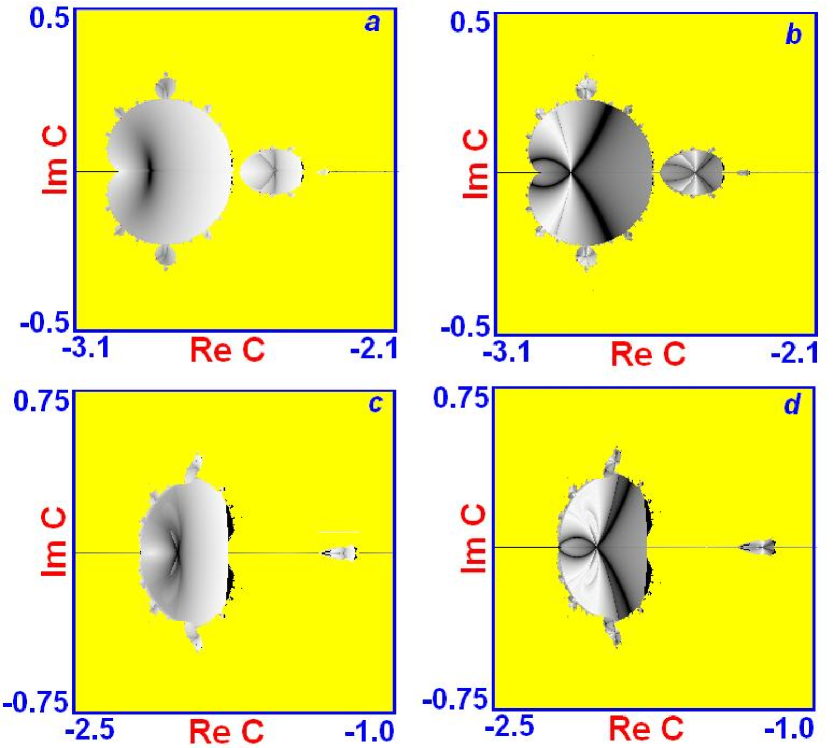
Figure 4: Charts of the largest Lyapunov exponent ($a$, $c$) and for the difference of the two larger exponents ($b$, $d$) for the ring system at the values of parameters, responsible for nonlinear mediae properties: $\alpha_{1}=0.01$, $\beta_{1}=1.0$, $\alpha_{2}=1.0$, $\beta_{2}=0.01$ ($a$, $b$) and $\alpha_{1}=0.05$, $\beta_{1}=1.0$, $\alpha_{2}=1.0$, $\beta_{2}=0.1$ ($c$, $d$). Values of other parameters are: $D=3$; $R_{1}=R_{2}=1.0$. Uniform color means area of unstable dynamics (divergence to infinity). Black color on the diagrams corresponds to chaotic dynamics in a bounded domain. More dark tone of gray color in the left column corresponds to smaller value of the senior Lyapunov exponent and more strong stability of the periodic regime. More dark tone of gray color in the right column means larger difference brtween Lyapuniv exponents and therefor more considerable distortion of the complex analyticity.

newpage

References

- [1] H.-O. Peitgen and P.H. Richter, The beauty of fractals. Images of complex dynamical systems, Springer-Verlag, New-York, 1986.
- [2] H.-O. Peitgen, H. Jurgens, and D. Saupe, Chaos and fractals: new frontiers of science, Springer-Verlag, New-York, 1992.
- [3] R.L. Devaney, An Introduction to chaotic dynamical systems, Addison-Wesley, New York, 1989.
- [4] C. Beck, Physical meaning for Mandelbrot and Julia set, Physica D125 (1999) 171-182.
- [5] O.B. Isaeva, On possibility of realization of the phenomena of complex analytical dynamics for the physical systems built up of coupled elements, which demonstrate period-doublings, Applied Nonlinear Dynamics (Saratov) 9 (6) (2001) 129-146 (in Russian).
- [6] O.B. Isaeva and S.P. Kuznetsov, On possibility of realization of the phenomena of complex analytic dynamics in physical systems. Novel mechanism of the synchronization loss in coupled period-doubling systems, Preprint http://xxx.lanl.gov/abs/nlin.CD/0509012.
- [7] O.B. Isaeva and S.P. Kuznetsov, On possibility of realization of the Mandelbrot set in coupled continuous systems, Preprint http://xxx.lanl.gov/abs/nlin.CD/0509013.
- [8] O.B. Isaeva, S.P. Kuznetsov, and V.I. Ponomarenko, Mandelbrot set in coupled logistic maps and in an electronic experiment, Phys. Rev. E64 (2001) 055201(R).
- [9] O.B. Isaeva, S.P. Kuznetsov and A.H. Osbaldestin, A system of alternately excited coupled non-autonomous oscillators manifesting phenomena intrinsic to complex analytical maps. Physica D237 (2008) 873-884.
- [10] K. Ikeda , H. Daido, O. Akimoto. Optical turbulence: chaotic behavior of transmitted light from a ring cavity. Phys. Pev. Lett. 45 (1980) 709.
- [11] A.M. Hagerstrom, W. Tong, M. Wu, B.A. Kalinikos and R. Eykholt. Excitation of chaotic spin waves in magnetic film feedback rings through three-wave nonlinear interactions. Phys. Rev. Lett. 102 (2009) 207202.
- [12] O.B. Isaeva, S.P. Kuznetsov and A.H. Osbaldestin. A system of alternately excited coupled non-autonomous oscillators manifesting phenomena intrinsic to complex analytical maps. Physica D, 237 (2008) 873-884.
- [13] G. Benettin, L. Galgani, A. Giorgilli and J.-M. Strelcyn, Lyapunov characteristic exponents for smooth dynamical systems and for Hamiltonian systems: A method for computing all of them. Part I: Theory. Part II: Numerical application, Meccanica 15 (1980) 9-30.
- [14] O.B. Isaeva and S.P. Kuznetsov, On scaling properties of two-dimensional maps near the accumulation point of the period-tripling cascade, Regular and Chaotic Dynamics 5 (4) (2000) 459-476.