Density functional theory on phase space

Abstract

Forty-five years after the point de départ [1] of density functional theory, its applications in chemistry and the study of electronic structures keep steadily growing. However, the precise form of the energy functional in terms of the electron density still eludes us – and possibly will do so forever [2]. In what follows we examine a formulation in the same spirit with phase space variables. The validity of Hohenberg–Kohn–Levy-type theorems on phase space is recalled. We study the representability problem for reduced Wigner functions, and proceed to analyze properties of the new functional. Along the way, new results on states in the phase space formalism of quantum mechanics are established. Natural Wigner orbital theory is developed in depth, with the final aim of constructing accurate correlation-exchange functionals on phase space. A new proof of the overbinding property of the Müller functional is given. This exact theory supplies its home at long last to that illustrious ancestor, the Thomas–Fermi model.

In memory of Jens Peder Dahl, dear friend and Wigner function’s stalwart

1 Introduction

1.1 Conventions and perspective

In this article Hartree atomic units [3] are used. The operator Hamiltonian $\mathbb{H}$ for $N$ fermions involves only one- and two-body observables. We work under the Born–Oppenheimer regime and look exclusively at the electronic problem, regarding the potential due to presence of nuclei as an external one. To fix ideas, consider the problem of $N$ electrons in an ion of charge $Z$ in the common approximation that neglects spin-orbit interaction and weaker couplings; so that in configuration space

$$\mathbb{H} =\sum_{i=1}^{N-1}\sum_{i<j}^{N}\mathbb{K}(\mkern-1.0mu{\vec{\mkern 1.0muq}}_{i},\mkern-1.0mu{\vec{\mkern 1.0muq}}_{j}):=\sum_{i=1}^{N-1}\sum_{j>i}^{N}\biggl{[}\frac{\mathrm{h}(\mkern-1.0mu{\vec{\mkern 1.0muq}}_{i})+\mathrm{h}(\mkern-1.0mu{\vec{\mkern 1.0muq}}_{j})}{N-1}+\frac{1}{|\mkern-1.0mu{\vec{\mkern 1.0muq}}_{i}-\mkern-1.0mu{\vec{\mkern 1.0muq}}_{j}|}\biggr{]}$$

$$:=\sum_{i=1}^{N-1}\sum_{j>i}^{N}\biggl{[}\biggl{(}-\frac{\Delta_{\mkern-1.0mu{\vec{\mkern 1.0muq}}_{i}}}{2}-\frac{Z}{|\mkern-1.0mu{\vec{\mkern 1.0muq}}_{i}|}-\frac{\Delta_{\mkern-1.0mu{\vec{\mkern 1.0muq}}_{j}}}{2}-\frac{Z}{|\mkern-1.0mu{\vec{\mkern 1.0muq}}_{j}|}\biggr{)}\frac{1}{N-1}+\frac{1}{|\mkern-1.0mu{\vec{\mkern 1.0muq}}_{i}-\mkern-1.0mu{\vec{\mkern 1.0muq}}_{j}|}\biggr{]}.$$

Remember that the set of all $N$-particle density matrices $D_{N}$ coincides with the set $\mathcal{D}^{N}$ of positive hermitian operators of unit trace on the Hilbert space of antisymmetric $N$-particle functions. This is a convex set, and its extreme elements are the pure states. When the system is in the (normalized) pure state $|\Psi_{N}\rangle$ the $N$-particle density matrix is of the form $D_{N}=|\Psi_{N}\rangle\langle\Psi_{N}|$; then $D_{N}^{2}=D_{N}$. Given $D_{N}$, one refers to the integral operator with kernel

$$D_{n}(1,\dots,n;1^{\prime},\dots,n^{\prime})=\int D_{N}(1,\dots,N;1^{\prime},\dots,n^{\prime},n+1,\dots,N)\,d(n+1)\dots dN$$ (1)

as the reduced $n$-matrix, or simply as the $n$-matrix. We denote by the same letter a $n$-matrix and its kernel and employ the standard notation $1=(\mkern-1.0mu{\vec{\mkern 1.0muq}}_{1},\varsigma_{1})$, and so on, for the spatial and spin variables. These reduced matrices are still positive operators with trace 1, but now they form only a proper subset of $\mathcal{D}^{n}$. The case $n=2$ is of special importance, since the energy of system takes the form

$$E=\binom{N}{2}\operatorname{tr}(\mathbb{K}D_{2}).$$ (2)

This is an exact linear functional of $D_{2}$, and the ground-state energy would be obtained by minimizing it on the set of 2-matrices. Therein lies the rub, as the $N$-representability problem for 2-matrices has never been efficiently solved [4]. This is why the Hohenberg–Kohn–Sham density functional theory (DFT) program [1] and its generalizations, initiated by the proof that the ground state density determines every property of an electronic system, still enjoy a tremendous success.

1.2 Purpose and plan of the article

This paper has the aim of sprucing up an untended corner of the garden of generalized density functional theories. The original DFT program is beset by our foreordained ignorance of the exact energy functional, while the reduced density matrix approach is hobbled by the unsolvability of the $N$-representability problem for two-electron densities. We push forward here the use of a quasidensity or quasiprobability on phase space, which is nothing other than the reduced single-body Wigner function, whose relation to 1-electron space $\rho(\mkern-1.0mu{\vec{\mkern 1.0muq}})$ and momentum $\pi(\mkern-1.0mu{\vec{\mkern 1.0mup}})$ densities is immediate.

Mathematically, Wigner functions [11, 12] are equivalent to density matrices; and in this sense our approach, dubbed Wigner density functional theory (WDFT), is equivalent to 1-density matrix functional theory. The beginnings of the latter go back to [13]; a surge of interest ensued, followed by a period of relative quiescence. More recently, this approach has seen a vigorous recent development centered around the notion of natural orbitals. However, WDFT can be worked out autonomously, calls for a different type of physical intuition, and readily lends itself to semi-classical treatments. Like one-body density matrix functional theory, it sits midway between ordinary DFT and the Coulson proposal of replacing the wave function by the 2-matrix [14]. It stands to contribute to (and to gain from) both the Kohn and Coulson programs.

Chief among our motivations is the success of the energetic program by Gill and coworkers – see for instance [15, 16] – to attack the problem of correlation energies via the family of Wigner intracules. Their method is rooted in the fundamental observation by Rassolov [17] that relative momentum is as important as relative position in determining interelectronic correlation; and this naturally calls for a phase space treatment.

Since we assume from the reader only basic familiarity with Wigner quasiprobabilities, we do most things from scratch, starting from a proof of the Rayleigh–Ritz principle in phase space quantum mechanics. After this, we give the main theorems for energy functionals based on the single-body Wigner function, in parallel with standard treatments. There we are brief, since arguments of this type have become routine.

The harmonium “atom” is treated exhaustively after that. Phase-space methods provide a fast lane towards an elegant and complete description of this system; it also serves as a training ground for employing the formalism.

True atomic Wigner functions are considered next. Phase-space eigenfunctions which are not quasidensities are needed for that. We characterize them for Gaussian basis wave functions; this result seems to be new. We perform some numerical atomic computations with those eigenfunctions.

Afterwards we (precisely define and) study natural Wigner orbitals. This is the heart of our subject. They come in handy to give a simpler proof than that of [18] of the “overbinding” property of the Müller 1-density matrix functional for helium. Again turning to harmonium, we illustrate with them the workings of exact functionals. The Shull–Löwdin–Kutzelnigg series is analytically summed here, for the first time as far as we know.

In Appendix A, we place the Thomas–Fermi (TF) models within our framework. The purpose is mainly pedagogical, illustrating how they fit harmoniously within WDFT. Another appendix elaborates on the characterization problem for Wigner functions.

The fundamental ideas of the present endeavour are found already in [19]; they appeared more developed in [20]. Włodarz came upon the same idea by the mid-nineties [21]. But apparently his paper had an almost negligible impact. It is perhaps prudent to clarify that our approach is not quite in the same spirit as the (then recent) work on a phase space distribution corresponding to a given electronic density $\rho$, reported in the texts [22, 23]. This had been conjured by Ghosh, Berkowitz and Parr [24, 25] by means of heuristic “local thermodynamics” arguments. The GBP Ansatz was put to good use [26, 27, 28] in the calculation of Compton profiles, exchange energies and corrections to the Thomas–Fermi–Dirac energy functional. Since the GBP distribution cannot be a true Wigner quasiprobability, its success should partially be attributed to the intrinsic strength of the phase space formalism.

There might be an issue of the use of Wigner quasiprobabilities versus other correspondences between ordinary quantum mechanics and $c$-numbers on phase space. Let it be said that, in the context of our quest, the mathematical advantages of Wigner functions are overwhelming. It would be difficult to develop natural orbital theory on phase space without the tracial property [30, 31] underlying (uniquely) the Wigner–Moyal correspondence, that allows for an almost verbatim translation of the spectral resolution for quantum states. Also the metaplectic invariance of this correspondence apparently is essential for the reconstruction of the 2-body Wigner function from the 1-body Wigner function for harmonium in Section 7.6. It lies behind generalized Wigner functions produced by fractional Fourier transforms [32], as well.

Last, but in no way least: this article seeks to continue and pay homage to outstanding work of many years by Dahl and Springborg (see [33, 34, 35] and references given later) on atomic and molecular Wigner functions, by addressing several matters of principle.

2 Classical Hamiltonians and Wigner functions

The Wigner quasiprobability corresponding to a density matrix $D_{N}$ is given by

$$P_{N}(\mkern-1.0mu{\vec{\mkern 1.0muq}}_{1},\dots,\mkern-1.0mu{\vec{\mkern 1.0muq}}_{N};\mkern-1.0mu{\vec{\mkern 1.0mup}}_{1},\dots,\mkern-1.0mu{\vec{\mkern 1.0mup}}_{N};\varsigma_{1},\dots,\varsigma_{N},\varsigma^{\prime}_{1},\dots,\varsigma^{\prime}_{N})$$

$$\qquad=\pi^{-3N}\int D_{N}(\mkern-1.0mu{\vec{\mkern 1.0muq}}_{1}-\mkern-1.0mu{\vec{\mkern 1.0muz}}_{1},\varsigma_{1},\dots,\mkern-1.0mu{\vec{\mkern 1.0muq}}_{N}-\mkern-1.0mu{\vec{\mkern 1.0muz}}_{N},\varsigma_{N};\mkern-1.0mu{\vec{\mkern 1.0muq}}_{1}+\mkern-1.0mu{\vec{\mkern 1.0muz}}_{1},\varsigma^{\prime}_{1},\dots,\mkern-1.0mu{\vec{\mkern 1.0muq}}_{N}+\mkern-1.0mu{\vec{\mkern 1.0muz}}_{N},\varsigma^{\prime}_{N})$$

$$\hskip 40.00006pt\times e^{2i(\mkern-1.0mu{\vec{\mkern 1.0mup}}_{1}\cdot\mkern-1.0mu{\vec{\mkern 1.0muz}}_{1}+\cdots+\mkern-1.0mu{\vec{\mkern 1.0mup}}_{N}\cdot\mkern-1.0mu{\vec{\mkern 1.0muz}}_{N})}\,d\mkern-1.0mu{\vec{\mkern 1.0muz}}_{1}\dots d\mkern-1.0mu{\vec{\mkern 1.0muz}}_{N}$$

$$\qquad=\pi^{-3N}\int D_{N}(1^{\prime},\dots,N^{\prime};1^{\prime\prime},\dots,N^{\prime\prime})e^{i(\mkern-1.0mu{\vec{\mkern 1.0mup}}_{1}\cdot(\mkern-1.0mu{\vec{\mkern 1.0muq}}^{\prime\prime}_{1}-\mkern-1.0mu{\vec{\mkern 1.0muq}}^{\prime}_{1})+\cdots+\mkern-1.0mu{\vec{\mkern 1.0mup}}_{N}\cdot(\mkern-1.0mu{\vec{\mkern 1.0muq}}^{\prime\prime}_{N}-\mkern-1.0mu{\vec{\mkern 1.0muq}}^{\prime}_{N}))}$$

$$\hskip 40.00006pt\times\delta\bigl{(}\mkern-1.0mu{\vec{\mkern 1.0muq}}_{1}-\tfrac{1}{2}(\mkern-1.0mu{\vec{\mkern 1.0muq}}^{\prime}_{1}+\mkern-1.0mu{\vec{\mkern 1.0muq}}^{\prime\prime}_{1})\bigr{)}\dots\delta\bigl{(}\mkern-1.0mu{\vec{\mkern 1.0muq}}_{N}-\tfrac{1}{2}(\mkern-1.0mu{\vec{\mkern 1.0muq}}^{\prime}_{N}+\mkern-1.0mu{\vec{\mkern 1.0muq}}^{\prime\prime}_{N})\bigr{)}\,d\mkern-1.0mu{\vec{\mkern 1.0muq}}^{\prime}_{1}\dots d\mkern-1.0mu{\vec{\mkern 1.0muq}}^{\prime}_{N}\,d\mkern-1.0mu{\vec{\mkern 1.0muq}}^{\prime\prime}_{1}\dots d\mkern-1.0mu{\vec{\mkern 1.0muq}}^{\prime\prime}_{N}.$$ (3)

This is symmetric under particle exchange. The definition extends to transitions $|\Psi_{N}\rangle\langle\Psi^{\prime}_{N}|$,

$$P_{\Psi_{N}\Psi^{\prime}_{N}}(\mkern-1.0mu{\vec{\mkern 1.0muq}}_{1},\dots,\mkern-1.0mu{\vec{\mkern 1.0muq}}_{N};\mkern-1.0mu{\vec{\mkern 1.0mup}}_{1},\dots,\mkern-1.0mu{\vec{\mkern 1.0mup}}_{N};\varsigma_{1},\dots,\varsigma_{N};\varsigma^{\prime}_{1},\dots,\varsigma^{\prime}_{N})$$

$$\qquad=\pi^{-3N}\int\Psi_{N}(\mkern-1.0mu{\vec{\mkern 1.0muq}}_{1}-\mkern-1.0mu{\vec{\mkern 1.0muz}}_{1},\varsigma_{1},\dots,\mkern-1.0mu{\vec{\mkern 1.0muq}}_{N}-\mkern-1.0mu{\vec{\mkern 1.0muz}}_{N},\varsigma_{N})\overline{\Psi^{\prime}}_{N}(\mkern-1.0mu{\vec{\mkern 1.0muq}}_{1}+\mkern-1.0mu{\vec{\mkern 1.0muz}}_{1},\varsigma^{\prime}_{1},\dots,\mkern-1.0mu{\vec{\mkern 1.0muq}}_{N}+\mkern-1.0mu{\vec{\mkern 1.0muz}}_{N},\varsigma^{\prime}_{N})$$

$$\hskip 40.00006pt\times e^{2i(\mkern-1.0mu{\vec{\mkern 1.0mup}}_{1}\cdot\mkern-1.0mu{\vec{\mkern 1.0muz}}_{1}+\cdots+\mkern-1.0mu{\vec{\mkern 1.0mup}}_{N}\cdot\mkern-1.0mu{\vec{\mkern 1.0muz}}_{N})}\,d\mkern-1.0mu{\vec{\mkern 1.0muz}}_{1}\dots d\mkern-1.0mu{\vec{\mkern 1.0muz}}_{N}.$$ (4)

We can regard Wigner quasiprobabilities as $2N\times 2N$ matrices on spin space. When there is no risk of confusion the corresponding spinless quantity, obtained by tracing on the spin variables, is denoted by the same name. Then hermiticity of $D_{N}$ in (3) translates into reality of $P_{N}$. The unit trace property translates into the normalization condition

$$\int P_{N}(\mkern-1.0mu{\vec{\mkern 1.0muq}}_{1},\dots,\mkern-1.0mu{\vec{\mkern 1.0muq}}_{N};\mkern-1.0mu{\vec{\mkern 1.0mup}}_{1},\dots,\mkern-1.0mu{\vec{\mkern 1.0mup}}_{N})\,d\mkern-1.0mu{\vec{\mkern 1.0muq}}_{1}\dots d\mkern-1.0mu{\vec{\mkern 1.0muq}}_{N}\,d\mkern-1.0mu{\vec{\mkern 1.0mup}}_{1}\dots d\mkern-1.0mu{\vec{\mkern 1.0mup}}_{N}=1.$$ (5)

Also, Wigner functions are square-summable and bounded continuous. By interpolation, $P_{N}\in L^{p}(\mathbb{R}^{6N})$ for all $2\leq p\leq\infty$. Notice that the above integral at any point of phase space is the expected value of a Grossmann–Royer parity observable [36, 37, 38]; those are Stratonovich–Weyl (de)quantizers on Kirillov coadjoint orbits [30, 31, 39]. Since a parity operator cannot have expectation value greater than 1, we note that

$$|P_{N}(\mkern-1.0mu{\vec{\mkern 1.0muq}}_{1},\dots,\mkern-1.0mu{\vec{\mkern 1.0muq}}_{N};\mkern-1.0mu{\vec{\mkern 1.0mup}}_{1},\dots,\mkern-1.0mu{\vec{\mkern 1.0mup}}_{N})|\leq\pi^{-3N},$$ (6)

with negative values being possible. This bound cannot be reached in more than one point, and in view of (5) it is often remarked that the support of a Wigner function is of bigger volume than $(h/2)^{3N}$. As a matter of fact, no square-summable Wigner function can have compact support in all of its variables, since then both the corresponding wavefunction and its Fourier transform would have compact support, which is impossible.

The distinctive trait of the phase space formulation is that expected values are calculated as phase space averages. Hence the classical observables reenter the quantum-mechanical game. Let $f$ be a real function of $\mkern-1.0mu{\vec{\mkern 1.0muq}}_{1},\dots,\mkern-1.0mu{\vec{\mkern 1.0muq}}_{N};\mkern-1.0mu{\vec{\mkern 1.0mup}}_{1},\dots,\mkern-1.0mu{\vec{\mkern 1.0mup}}_{N}$ (a symbol) and let $\mathbb{Q}(f)$ be its quantized operator version (by the Weyl rule). We work with symbols symmetric in their arguments. Then we get:

$$\operatorname{tr}\bigl{(}\mathbb{Q}(f)D_{N}\bigr{)}=\int f(\mkern-1.0mu{\vec{\mkern 1.0muq}}_{1},\dots,\mkern-1.0mu{\vec{\mkern 1.0muq}}_{N};\mkern-1.0mu{\vec{\mkern 1.0mup}}_{1},\dots,\mkern-1.0mu{\vec{\mkern 1.0mup}}_{N})P_{N}(\mkern-1.0mu{\vec{\mkern 1.0muq}}_{1},\dots,\mkern-1.0mu{\vec{\mkern 1.0muq}}_{N};\mkern-1.0mu{\vec{\mkern 1.0mup}}_{1},\dots,\mkern-1.0mu{\vec{\mkern 1.0mup}}_{N})\,\,d\mkern-1.0mu{\vec{\mkern 1.0muq}}_{1}\dots d\mkern-1.0mu{\vec{\mkern 1.0muq}}_{N}\,d\mkern-1.0mu{\vec{\mkern 1.0mup}}_{1}\dots d\mkern-1.0mu{\vec{\mkern 1.0mup}}_{N}.$$

One must keep in mind that the symbol for the operator $D_{N}$ is not $P_{N}$, but $(2\pi)^{3N}P_{N}=:W_{N}$. That is, $\mathbb{Q}(P_{N})=D_{N}/(2\pi)^{3N}$. A Wigner quasiprobability behaves in almost every way like a probability density on phase space, except that in general is not nonnegative everywhere. It is not so easy, however, to recognize quantum state representatives among all functions on phase space: see Appendix B.

2.1 Reduced Wigner functions

Reduced Wigner quasiprobabilities, up to and including the single-particle quasidensity $d$ on phase space, are obtained in the obvious way by integrating successively over groups of 6 variables. In particular:

$$d_{2}(\mkern-1.0mu{\vec{\mkern 1.0muq}}_{1},\mkern-1.0mu{\vec{\mkern 1.0muq}}_{2};\mkern-1.0mu{\vec{\mkern 1.0mup}}_{1},\mkern-1.0mu{\vec{\mkern 1.0mup}}_{2};\varsigma_{1},\varsigma_{2};\varsigma^{\prime}_{1},\varsigma^{\prime}_{2})$$

$$\qquad:=\frac{N(N-1)}{2}\int P_{N}(\mkern-1.0mu{\vec{\mkern 1.0muq}}_{1},\mkern-1.0mu{\vec{\mkern 1.0muq}}_{2},\mkern-1.0mu{\vec{\mkern 1.0muq}}_{3}\dots,\mkern-1.0mu{\vec{\mkern 1.0muq}}_{N};\mkern-1.0mu{\vec{\mkern 1.0mup}}_{1},\mkern-1.0mu{\vec{\mkern 1.0mup}}_{2},\mkern-1.0mu{\vec{\mkern 1.0mup}}_{3}\dots,\mkern-1.0mu{\vec{\mkern 1.0mup}}_{N};\varsigma_{1},\varsigma_{2},\varsigma_{3},\dots,\varsigma_{N};\varsigma^{\prime}_{1},\varsigma^{\prime}_{2},\varsigma_{3}\dots,\varsigma_{N})$$

$$\hskip 40.00006ptd\mkern-1.0mu{\vec{\mkern 1.0muq}}_{3}\dots d\mkern-1.0mu{\vec{\mkern 1.0muq}}_{N}\,d\mkern-1.0mu{\vec{\mkern 1.0mup}}_{3}\dots d\mkern-1.0mu{\vec{\mkern 1.0mup}}_{N}\,d\varsigma_{3}\dots d\varsigma_{N};$$

$$d(\mkern-1.0mu{\vec{\mkern 1.0muq}};\mkern-1.0mu{\vec{\mkern 1.0mup}};\varsigma;\varsigma^{\prime})\equiv d_{1}(\mkern-1.0mu{\vec{\mkern 1.0muq}};\mkern-1.0mu{\vec{\mkern 1.0mup}};\varsigma;\varsigma^{\prime}):=\frac{2}{N-1}\int d_{2}(\mkern-1.0mu{\vec{\mkern 1.0muq}},\mkern-1.0mu{\vec{\mkern 1.0muq}}_{2};\mkern-1.0mu{\vec{\mkern 1.0mup}},\mkern-1.0mu{\vec{\mkern 1.0mup}}_{2};\varsigma,\varsigma_{2};\varsigma^{\prime},\varsigma_{2})\,d\mkern-1.0mu{\vec{\mkern 1.0muq}}_{2}\,d\mkern-1.0mu{\vec{\mkern 1.0mup}}_{2}\,d\varsigma_{2}.$$ (7)

By partial integration of $d$ one gets the 1-electron density $\rho$ and momentum density $\pi$:

$$\rho(\mkern-1.0mu{\vec{\mkern 1.0muq}})=\int d(\mkern-1.0mu{\vec{\mkern 1.0muq}};\mkern-1.0mu{\vec{\mkern 1.0mup}};\varsigma;\varsigma)\,d\mkern-1.0mu{\vec{\mkern 1.0mup}}\,d\varsigma;\qquad\pi(\mkern-1.0mu{\vec{\mkern 1.0mup}})=\int d(\mkern-1.0mu{\vec{\mkern 1.0muq}};\mkern-1.0mu{\vec{\mkern 1.0mup}};\varsigma;\varsigma)\,d\mkern-1.0mu{\vec{\mkern 1.0muq}}\,d\varsigma.$$ (8)

Also the form factors are easily expressed in terms of $d_{1}$. Since dequantization and reduction commute, we may also use formulas analogous to (3) for reduced density matrices. At each order the reduced Wigner distributions contain the same information as the corresponding reduced density matrices. It is convenient to have “inversion formulas” to recover the latter matrices from the Wigner functions. It transpires that

$$\Gamma(1,2;1^{\prime},2^{\prime}) =\int d_{2}\Bigl{(}\frac{\mkern-1.0mu{\vec{\mkern 1.0muq}}_{1}+\mkern-1.0mu{\vec{\mkern 1.0muq}}^{\prime}_{1}}{2},\frac{\mkern-1.0mu{\vec{\mkern 1.0muq}}_{2}+\mkern-1.0mu{\vec{\mkern 1.0muq}}^{\prime}_{2}}{2};\mkern-1.0mu{\vec{\mkern 1.0mup}}_{1},\mkern-1.0mu{\vec{\mkern 1.0mup}}_{2};\varsigma_{1},\varsigma_{2};\varsigma^{\prime}_{1},\varsigma^{\prime}_{2}\Bigr{)}e^{i(\mkern-1.0mu{\vec{\mkern 1.0mup}}_{1}\cdot(\mkern-1.0mu{\vec{\mkern 1.0muq}}_{1}-\mkern-1.0mu{\vec{\mkern 1.0muq}}^{\prime}_{1})+\mkern-1.0mu{\vec{\mkern 1.0mup}}_{2}\cdot(\mkern-1.0mu{\vec{\mkern 1.0muq}}_{2}-\mkern-1.0mu{\vec{\mkern 1.0muq}}^{\prime}_{2}))}\,d\mkern-1.0mu{\vec{\mkern 1.0mup}}_{1}\,d\mkern-1.0mu{\vec{\mkern 1.0mup}}_{2},$$

$$\gamma(1;1^{\prime}) =\int d\Bigl{(}\frac{\mkern-1.0mu{\vec{\mkern 1.0muq}}+\mkern-1.0mu{\vec{\mkern 1.0muq}}^{\prime}}{2};\mkern-1.0mu{\vec{\mkern 1.0mup}};\varsigma;\varsigma^{\prime}\Bigr{)}e^{i\mkern-1.0mu{\vec{\mkern 1.0mup}}\cdot(\mkern-1.0mu{\vec{\mkern 1.0muq}}-\mkern-1.0mu{\vec{\mkern 1.0muq}}^{\prime})}\,d\mkern-1.0mu{\vec{\mkern 1.0mup}},$$ (9)

where $\Gamma=\tfrac{1}{2}N(N-1)D_{2}$ and $\gamma=ND_{1}$ as usually defined in quantum chemistry. (Note that $d_{2}$ corresponds to $\Gamma$ rather than to $D_{2}$ and $d_{1}$ to $\gamma$ rather than to $D_{1}$.)

One may usefully translate Coleman’s theorems [4] on representable 1-density matrices into properties of $d$. This was done by Harriman [40]. Let $\mathcal{D}^{1}_{N}$ denote the set of 1-matrices representable by (1); it happens that $\mathcal{D}^{1}_{N}\subsetneq\mathcal{D}^{1}$. In fact, $d$ is the 1-body Wigner quasidensity corresponding to an element of $\mathcal{D}^{1}_{N}$ if and only if

$$0\leq\int W(\mkern-1.0mu{\vec{\mkern 1.0muq}};\mkern-1.0mu{\vec{\mkern 1.0mup}})d(\mkern-1.0mu{\vec{\mkern 1.0muq}};\mkern-1.0mu{\vec{\mkern 1.0mup}})\,d\mkern-1.0mu{\vec{\mkern 1.0muq}}\,d\mkern-1.0mu{\vec{\mkern 1.0mup}}\leq 2$$ (10)

for any $W$ which is the symbol of an arbitrary element of $\mathcal{D}^{1}$. Recall that $d$ may be regarded as a $2\times 2$ matrix in spin space. We can write for instance,

$$d(\mkern-1.0mu{\vec{\mkern 1.0muq}};\mkern-1.0mu{\vec{\mkern 1.0mup}};\varsigma,\varsigma^{\prime})=\begin{pmatrix}d_{{\mathord{\uparrow}}{\mathord{\uparrow}}}(\mkern-1.0mu{\vec{\mkern 1.0muq}};\mkern-1.0mu{\vec{\mkern 1.0mup}})&d_{{\mathord{\uparrow}}{\mathord{\downarrow}}}(\mkern-1.0mu{\vec{\mkern 1.0muq}};\mkern-1.0mu{\vec{\mkern 1.0mup}})\\ d_{{\mathord{\downarrow}}{\mathord{\uparrow}}}(\mkern-1.0mu{\vec{\mkern 1.0muq}};\mkern-1.0mu{\vec{\mkern 1.0mup}})&d_{{\mathord{\downarrow}}{\mathord{\downarrow}}}(\mkern-1.0mu{\vec{\mkern 1.0muq}};\mkern-1.0mu{\vec{\mkern 1.0mup}})\end{pmatrix};$$

and $d(\mkern-1.0mu{\vec{\mkern 1.0muq}};\mkern-1.0mu{\vec{\mkern 1.0mup}})$ in (10) means the trace of $d(\mkern-1.0mu{\vec{\mkern 1.0muq}};\mkern-1.0mu{\vec{\mkern 1.0mup}};\varsigma,\varsigma^{\prime})$ – or its scalar part, in a more cogent specification of $d$ according to the behaviour of its components under rotation. Analogously $d_{2}$ may be regarded as a $4\times 4$ matrix in spin space or as a direct sum of higher tensor representations of the rotation group. The Ayers trick – see [6] for instance – is easily reformulated here: the 1-body Wigner quasidensity belongs to $\mathcal{D}^{1}_{N}$ if and only if

$$\int h(\mkern-1.0mu{\vec{\mkern 1.0muq}};\mkern-1.0mu{\vec{\mkern 1.0mup}})d(\mkern-1.0mu{\vec{\mkern 1.0muq}};\mkern-1.0mu{\vec{\mkern 1.0mup}})\,d\mkern-1.0mu{\vec{\mkern 1.0muq}}\,d\mkern-1.0mu{\vec{\mkern 1.0mup}}\geq E_{0}[h;N]$$

for every 1-body potential $h(\mkern-1.0mu{\vec{\mkern 1.0muq}};\mkern-1.0mu{\vec{\mkern 1.0mup}})$, where $E_{0}[h;N]$ denotes the ground state energy of $N$ fermions under such potential; likewise the 2-body Wigner quasidensity $d_{2}$ is $N$-representable if and only if

$$\int h_{2}(\mkern-1.0mu{\vec{\mkern 1.0muq}}_{1},\mkern-1.0mu{\vec{\mkern 1.0muq}}_{2};\mkern-1.0mu{\vec{\mkern 1.0mup}}_{1},\mkern-1.0mu{\vec{\mkern 1.0mup}}_{2})d_{2}(\mkern-1.0mu{\vec{\mkern 1.0muq}}_{1},\mkern-1.0mu{\vec{\mkern 1.0muq}}_{2};\mkern-1.0mu{\vec{\mkern 1.0mup}}_{1},\mkern-1.0mu{\vec{\mkern 1.0mup}}_{2})\,d\mkern-1.0mu{\vec{\mkern 1.0muq}}_{1}\,d\mkern-1.0mu{\vec{\mkern 1.0mup}}_{1}\,d\mkern-1.0mu{\vec{\mkern 1.0muq}}_{2}\,d\mkern-1.0mu{\vec{\mkern 1.0mup}}_{2}\geq E_{0}[h_{2};N]$$

for any 2-body Hamiltonian $h_{2}$. The “only if” part is clear, for otherwise the variational principle would be violated. The “if” part requires the Hahn–Banach theorem.

The quasidensity corresponding to a Slater determinant (that is, an extremal element of $\mathcal{D}^{1}_{N}$) is the sum with equal weight 1 of the contributions of the occupied orbitals [34]:

$$d(\mkern-1.0mu{\vec{\mkern 1.0muq}};\mkern-1.0mu{\vec{\mkern 1.0mup}};\varsigma;\varsigma^{\prime})=\sum_{i=1}^{N}f_{i}(\mkern-1.0mu{\vec{\mkern 1.0muq}};\mkern-1.0mu{\vec{\mkern 1.0mup}};\varsigma;\varsigma^{\prime}),$$

with the $f_{i}$ being (mutually orthogonal) pure-state Wigner functions. Note, as well, that in this case

$$\int d(\mkern-1.0mu{\vec{\mkern 1.0muq}};\mkern-1.0mu{\vec{\mkern 1.0mup}})^{2}\,d\mkern-1.0mu{\vec{\mkern 1.0muq}}\,d\mkern-1.0mu{\vec{\mkern 1.0mup}}=\frac{2N}{(2\pi)^{3}}.$$ (11)

In summary, quasidensities look like mixed-state Wigner quasiprobabilities. Typically, the latter are “less negative” than Wigner functions representing pure states.

2.2 Spectral theorem and variational principle on phase space

The spectral theorem for phase space quantum mechanics was given in [41, 42]. Its formulation demands the concept of Moyal or twisted product $\times$, indirectly defined by $\mathbb{Q}(f\times g)=\mathbb{Q}(f)\mathbb{Q}(g)$. To alleviate notation in what follows we employ the convention $q=(\mkern-1.0mu{\vec{\mkern 1.0muq}}_{1},\dots,\mkern-1.0mu{\vec{\mkern 1.0muq}}_{N})$, and similarly for the other variables. The twisted product is

$$f\times g(q;p)=\int f(q^{\prime};p^{\prime})g(q^{\prime\prime};p^{\prime\prime})\exp[2i(qp^{\prime}-q^{\prime}p+q^{\prime}p^{\prime\prime}-q^{\prime\prime}p^{\prime}+q^{\prime\prime}p-qp^{\prime\prime})]\,\frac{dq^{\prime}\,dp^{\prime}\,dq^{\prime\prime}\,dp^{\prime\prime}}{\pi^{6N}},$$

with the properties:

$$\int f\times g(q;p)\,dq\,dp=\int f(q;p)g(q;p)\,dq\,dp=\int g\times f(q;p)\,dq\,dp;\quad\overline{f\times g}=\overline{g}\times\overline{f}.$$ (12)

Theorem 1.

Assume for simplicity a purely discrete nondegenerate energy spectrum $E_{0}<E_{1}<\cdots<E_{n}<\cdots$. Then:

• The solutions $\Gamma_{nm}$, for $n,m=0,1,2,\dots$, of the simultaneous eigenvalue equations:

  $$H\times\Gamma_{nm}=E_{n}\,\Gamma_{nm},\qquad\Gamma_{nm}\times H=E_{m}\,\Gamma_{nm},$$ (13)

  form a doubly indexed orthogonal basis for the space of functions on phase space. These functions describe stationary states when $n=m$; when $n\neq m$ they describe transitions between pairs of states. Note that $\Gamma_{nm}=\overline{\Gamma_{mn}}$ by (12).

• The sequence of those eigenvalues gives precisely the spectrum of $H$.

• With the normalization

  $$\int|\Gamma_{nm}|^{2}\,\frac{dq\,dp}{(2\pi)^{3N}}=1,$$

  we obtain

  $$\Gamma_{nm}\times\Gamma_{kl}=\Gamma_{nl}\,\delta_{mk}\quad\mbox{and the identity}\quad\int\Gamma_{mn}(q;p)\,\frac{dq\,dp}{(2\pi)^{3N}}=\delta_{mn},$$ (14)

  consistently with (12) and (13). Clearly $\Gamma_{nn}/(2\pi)^{3N}$ is the Wigner quasiprobability corresponding to the state of energy $E_{n}$.

• Also, the following closure relations hold:

  $$\sum_{n}\Gamma_{nn}(q;p)=1;\qquad\sum_{m,n}\Gamma_{nm}(q;p)\Gamma_{mn}(q^{\prime};p^{\prime})=(2\pi)^{3N}\,\delta(q-q^{\prime})\,\delta(p-p^{\prime}).$$

• Finally, we can write

  $$H=\sum_{n}E_{n}\,\Gamma_{nn}.$$

Corollary 2.

For any normalized state $P_{N}$ and any Hamiltonian $H$, if $E_{0}$ denotes the energy of the ground state corresponding to $H$, then:

$$E_{0}\leq\int H(q;p)P_{N}(q;p)\,dq\,dp.$$

Equality is reached if and only if $P_{N}=P_{\mathrm{gs}}$, the Wigner distribution for the ground state.

The validity of this variational principle is of course not restricted to electronic systems.

Proof.

Any function $F$ of the phase space variables may be expanded in a double series of eigentransitions corresponding to $H$. In particular,

$$P_{N}=\sum_{m,n}c_{mn}\Gamma_{mn},$$ (15)

where:

$$c_{mn}=\int P_{N}(q;p)\Gamma_{nm}(q;p)\,\frac{dq\,dp}{(2\pi)^{3N}}.$$

Thus

$$\int H(q;p)P_{N}(q;p)\,\frac{dq\,dp}{(2\pi)^{3N}}=\int(H\times P_{N})(q;p)\,\frac{dq\,dp}{(2\pi)^{3N}}=\sum_{n}E_{n}\,c_{nn},$$

where we have used (12), (14) and (15). Now take for $F$ the symbol $W_{N}$ of a pure state, so that $W_{N}=W_{N}\times W_{N}$. An immediate calculation gives $c_{nn}=\sum_{m}|c_{mn}|^{2}\geq 0$. The rest is obvious. ∎

3 The main theorems

Let us invoke the classical Hamiltonian of an electronic system under the form:

$$H=T+V_{\mathrm{ee}}+V_{\mathrm{ext}},$$ (16)

where

$$T=\sum_{i=1}^{N}\frac{|\mkern-1.0mu{\vec{\mkern 1.0mup}}_{i}|^{2}}{2};\qquad V_{\mathrm{ee}}=\sum_{i<j}\frac{1}{|\mkern-1.0mu{\vec{\mkern 1.0muq}}_{i}-\mkern-1.0mu{\vec{\mkern 1.0muq}}_{j}|};\qquad V_{\mathrm{ext}}=\sum_{i=1}^{N}V(\mkern-1.0mu{\vec{\mkern 1.0muq}}_{i};\mkern-1.0mu{\vec{\mkern 1.0mup}}_{i}).$$

Here $V_{\mathrm{ext}}$ denotes the external “potential” (e.g., due to the nucleus in an atom plus an external magnetic field). It is clear that the energy of a $N$-electronic system is a functional of $d_{2}$. But we can prove more.

Theorem 3.

The many-body ground state of the system is determined by its 1-body quasidensity.

Proof.

Like in DFT, we argue by contradiction. Suppose that we have two different (by more than a constant) external potentials $V_{\mathrm{ext}}$, $V^{\prime}_{\mathrm{ext}}$ acting on our electronic system, with corresponding ground Wigner states $P_{\mathrm{gs}}$, $P^{\prime}_{\mathrm{gs}}$ (assumed different) and respective ground state energies $E_{0}$, $E^{\prime}_{0}$, whose associated 1-body quasidensity is the same. Then, by the variational principle on phase space of the previous section, we get

$$E^{\prime}_{0} =\int H^{\prime}P^{\prime}_{\mathrm{gs}}\,dq\,dp<\int H^{\prime}P_{\mathrm{gs}}\,dq\,dp$$

$$=\int(H+V^{\prime}_{\mathrm{ext}}-V_{\mathrm{ext}})P_{\mathrm{gs}}\,dq\,dp=E_{0}+\int(V^{\prime}_{\mathrm{ext}}-V_{\mathrm{ext}})P_{\mathrm{gs}}\,dq\,dp.$$

But

$$\int(V^{\prime}_{\mathrm{ext}}-V_{\mathrm{ext}})P_{\mathrm{gs}}\,dq\,dp=\int(V^{\prime}_{\mathrm{ext}}-V_{\mathrm{ext}})(\mkern-1.0mu{\vec{\mkern 1.0muq}};\mkern-1.0mu{\vec{\mkern 1.0mup}})\,d_{\mathrm{gs}}(\mkern-1.0mu{\vec{\mkern 1.0muq}};\mkern-1.0mu{\vec{\mkern 1.0mup}})\,d\mkern-1.0mu{\vec{\mkern 1.0muq}}\,d\mkern-1.0mu{\vec{\mkern 1.0mup}}.$$

The same argument shows that

$$E_{0}<E^{\prime}_{0}+\int(V_{\mathrm{ext}}-V^{\prime}_{\mathrm{ext}})(\mkern-1.0mu{\vec{\mkern 1.0muq}};\mkern-1.0mu{\vec{\mkern 1.0mup}})\,d_{\mathrm{gs}}(\mkern-1.0mu{\vec{\mkern 1.0muq}};\mkern-1.0mu{\vec{\mkern 1.0mup}})\,d\mkern-1.0mu{\vec{\mkern 1.0muq}}\,d\mkern-1.0mu{\vec{\mkern 1.0mup}}.$$

and we obtain a contradiction. Thus $d_{\mathrm{gs}}$ fixes $P_{\mathrm{gs}}$ (and thereby the expected value of any observable in the ground state). ∎

Next we avoid $V$-representability problems by a constrained-search definition of the energy functional.

Theorem 4.

There exists a functional $\mathcal{A}$ of the electronic quasiprobability $d$, such that:

$$E_{0}\leq\int V(\mkern-1.0mu{\vec{\mkern 1.0muq}};\mkern-1.0mu{\vec{\mkern 1.0mup}})d(\mkern-1.0mu{\vec{\mkern 1.0muq}};\mkern-1.0mu{\vec{\mkern 1.0mup}})\,d\mkern-1.0mu{\vec{\mkern 1.0muq}}\,d\mkern-1.0mu{\vec{\mkern 1.0mup}}+\int\frac{|\mkern-1.0mu{\vec{\mkern 1.0mup}}|^{2}}{2}\,d(\mkern-1.0mu{\vec{\mkern 1.0muq}};\mkern-1.0mu{\vec{\mkern 1.0mup}})\,d\mkern-1.0mu{\vec{\mkern 1.0muq}}\,d\mkern-1.0mu{\vec{\mkern 1.0mup}}+\mathcal{A}[d]=:\mathcal{E}[d].$$

Moreover, if $d_{\mathrm{gs}}$ is the quasidensity corresponding to the ground state, then:

$$E_{0}=\int V(\mkern-1.0mu{\vec{\mkern 1.0muq}},\mkern-1.0mu{\vec{\mkern 1.0mup}})d_{\mathrm{gs}}(\mkern-1.0mu{\vec{\mkern 1.0muq}},\mkern-1.0mu{\vec{\mkern 1.0mup}})\,d\mkern-1.0mu{\vec{\mkern 1.0muq}}\,d\mkern-1.0mu{\vec{\mkern 1.0mup}}+\int\frac{|\mkern-1.0mu{\vec{\mkern 1.0mup}}|^{2}}{2}\,d_{\mathrm{gs}}(\mkern-1.0mu{\vec{\mkern 1.0muq}},\mkern-1.0mu{\vec{\mkern 1.0mup}})\,d\mkern-1.0mu{\vec{\mkern 1.0muq}}\,d\mkern-1.0mu{\vec{\mkern 1.0mup}}+\mathcal{A}(d_{\mathrm{gs}})=\mathcal{E}(d_{\mathrm{gs}}).$$

Proof.

Let $\mathcal{A}[d]$ be

$$\min\int P_{d}(q;p)V_{\mathrm{ee}}(q;p)\,dq\,dp,$$ (17)

where $P_{d}$ runs through every Wigner $N$-distribution (representing mixed states in general) giving the fixed quasidensity $d$. Let $P_{d}^{\mathrm{min}}$ be the one attaining this minimum. (Such $P_{d}$ form a compact convex set, with respect to a topology that makes $P_{d}\mapsto\int P_{d}V_{\mathrm{ee}}$ a continuous linear form, so its minimum will be attained.) The variational principle says that

$$\int V(\mkern-1.0mu{\vec{\mkern 1.0muq}};\mkern-1.0mu{\vec{\mkern 1.0mup}})d(\mkern-1.0mu{\vec{\mkern 1.0muq}};\mkern-1.0mu{\vec{\mkern 1.0mup}})\,d\mkern-1.0mu{\vec{\mkern 1.0muq}}\,d\mkern-1.0mu{\vec{\mkern 1.0mup}}+\int\frac{|\mkern-1.0mu{\vec{\mkern 1.0mup}}|^{2}}{2}\pi(\mkern-1.0mu{\vec{\mkern 1.0mup}})\,d\mkern-1.0mu{\vec{\mkern 1.0mup}}+\mathcal{A}[d]=\int H(q;p)P_{d}^{\mathrm{min}}(q;p)\,dq\,dp\geq E_{0}.$$ (18)

In particular,

$$E_{0}=\int H(q;p)P_{\mathrm{gs}}(q;p)\,dq\,dp\leq\int H(q;p)P_{d_{\mathrm{gs}}}^{\mathrm{min}}(q;p)\,dq\,dp.$$

This gives

$$\int P_{\mathrm{gs}}(q;p)V_{\mathrm{ee}}(q;p)\,dq\,dp\leq\int P_{d_{\mathrm{gs}}}^{\mathrm{min}}(q;p)V_{\mathrm{ee}}(q;p)\,dq\,dp.$$

On the other hand, by definition, the reverse inequality holds:

$$\int P_{d_{\mathrm{gs}}}^{\mathrm{min}}(q;p)V_{\mathrm{ee}}(q;p)\,dq\,dp\leq\int P_{\mathrm{gs}}(q;p)V_{\mathrm{ee}}(q;p)\,dq\,dp.$$ ∎

The minimization has been carried out in two stages. First we perform a search constrained by the trial quasidensity $d$. In the second step, expression (18) is minimized. By Corollary 2, $P_{\mathrm{gs}}=P_{d_{\mathrm{gs}}}^{\mathrm{min}}$, which means that $P_{\mathrm{gs}}$ can be obtained from $P^{\mathrm{min}}_{d_{\mathrm{gs}}}$ directly even if the external potential is unknown. As in Levy’s formulation of the Hohenberg–Kohn functional [43], $\mathcal{A}$ is universal, i.e., independent of $V$; nor is a ground state $V$-representability condition required. Thus our variational principle escapes the major problems of the original DFT one – see the discussion in [44, Chap. 33]. Systems with external potentials depending on momenta (as with orbital magnetism) fall into its purvey. Also, in the variation above we need not restrict to one-body Wigner quasiprobabilities corresponding to pure states; only finiteness conditions, such as that $d$ should belong to the domain of the kinetic energy,

$$T[d]=\int\frac{|\mkern-1.0mu{\vec{\mkern 1.0mup}}|^{2}}{2}\,d(\mkern-1.0mu{\vec{\mkern 1.0muq}};\mkern-1.0mu{\vec{\mkern 1.0mup}})\,d\mkern-1.0mu{\vec{\mkern 1.0muq}}\,d\mkern-1.0mu{\vec{\mkern 1.0mup}}<\infty,$$ (19)

are implicit. Thus our apparent restriction to nondegenerate ground states is merely an inessential notational simplification: WDFT is an ensemble functional theory able to deal with degenerate ground states. For the same reason, $\mathcal{A}[d]$ is a convex functional, and therefore $\mathcal{E}[d]$ too is convex.

3.1 Exact requisites for the quasidensity functional

In this subsection we collect a number of properties and conditions on $\mathcal{A}[d]$ within exact WDFT.

• A Legendre transform variant of $\mathcal{A}$ exists:

  $$\mathcal{A}_{L}[d]=\sup\Bigl{[}E[V_{\mathrm{ext}}]-\int\bigl{(}\tfrac{1}{2}|\mkern-1.0mu{\vec{\mkern 1.0mup}}|^{2}+V_{\mathrm{ext}}(\mkern-1.0mu{\vec{\mkern 1.0muq}};\mkern-1.0mu{\vec{\mkern 1.0mup}})\bigr{)}d(\mkern-1.0mu{\vec{\mkern 1.0muq}};\mkern-1.0mu{\vec{\mkern 1.0mup}})\,d\mkern-1.0mu{\vec{\mkern 1.0muq}}\,d\mkern-1.0mu{\vec{\mkern 1.0mup}}\,\Bigr{]}.$$

  The supremum is taken over all possible choices of the external potential. The Legendre transform allows a reformulation of the previous variational theorems, in the spirit of [45].

• Let $V_{\mathrm{ext}}$ depend on a parameter $\lambda$. Then we denote the Hamiltonian by $H_{\lambda}$. Consider the associated eigenvalue problem:

  $$H_{\lambda}\times\Gamma_{\lambda}=E_{\lambda}\,\Gamma_{\lambda}=\Gamma_{\lambda}\times H_{\lambda},$$

  with $\Gamma_{\lambda}$ being a normalized Wigner distribution. The assertion that

  $$\frac{dE_{\lambda}}{d\lambda}=\int\frac{\partial H_{\lambda}(q;p)}{\partial\lambda}\,\Gamma_{\lambda}(q;p)\,dq\,dp$$ (20)

  is the Hellmann–Feynman theorem in phase space quantum mechanics.

  Proof.

  Indeed, $E_{\lambda}=\int H_{\lambda}(q;p)\,\Gamma_{\lambda}(q;p)\,dq\,dp$ implies

  $$\frac{dE_{\lambda}}{d\lambda}=\int\frac{\partial H_{\lambda}(q;p)}{\partial\lambda}\,\Gamma_{\lambda}(q;p)\,dq\,dp+\int H_{\lambda}(q;p)\,\frac{\partial\Gamma_{\lambda}(q;p)}{\partial\lambda}\,dq\,dp.$$

  However,

  $$\int\!H_{\lambda}(q;p)\,\frac{\partial\Gamma_{\lambda}(q;p)}{\partial\lambda}\,dq\,dp=\int\!H_{\lambda}(q;p)\times\frac{\partial\Gamma_{\lambda}(q;p)}{\partial\lambda}\,dq\,dp=E_{\lambda}\int\frac{\partial\Gamma_{\lambda}(q;p)}{\partial\lambda}\,dq\,dp=0.$$

  The theorem follows. ∎

• Now, let us write

  $$V_{\mathrm{ext},\lambda}(\mkern-1.0mu{\vec{\mkern 1.0muq}};\mkern-1.0mu{\vec{\mkern 1.0mup}})=V_{\mathrm{ext}}(\mkern-1.0mu{\vec{\mkern 1.0muq}};\mkern-1.0mu{\vec{\mkern 1.0mup}})+\lambda\mkern-1.0mu{\vec{\mkern 1.0mur}}_{1}\cdot\nabla_{\!\mkern-1.0mu{\vec{\mkern 1.0muq}}}V_{\mathrm{ext}}(\mkern-1.0mu{\vec{\mkern 1.0muq}};\mkern-1.0mu{\vec{\mkern 1.0mup}})+\lambda\mkern-1.0mu{\vec{\mkern 1.0mur}}_{2}\cdot\nabla_{\!\mkern-1.0mu{\vec{\mkern 1.0mup}}}V_{\mathrm{ext}}(\mkern-1.0mu{\vec{\mkern 1.0muq}};\mkern-1.0mu{\vec{\mkern 1.0mup}})+\cdots$$

  for arbitrary vectors $\mkern-1.0mu{\vec{\mkern 1.0mur}}_{1},\mkern-1.0mu{\vec{\mkern 1.0mur}}_{2}$. Thus, by (20) and homogeneity of space,

  $$\int d(\mkern-1.0mu{\vec{\mkern 1.0muq}};\mkern-1.0mu{\vec{\mkern 1.0mup}})(\nabla_{\!\mkern-1.0mu{\vec{\mkern 1.0muq}}}+\nabla_{\!\mkern-1.0mu{\vec{\mkern 1.0mup}}})V_{\mathrm{ext}}(\mkern-1.0mu{\vec{\mkern 1.0muq}};\mkern-1.0mu{\vec{\mkern 1.0mup}})\,d\mkern-1.0mu{\vec{\mkern 1.0muq}}\,d\mkern-1.0mu{\vec{\mkern 1.0mup}}=0.$$

  Similarly, by isotropy of space,

  $$\int d(\mkern-1.0mu{\vec{\mkern 1.0muq}};\mkern-1.0mu{\vec{\mkern 1.0mup}})(\mkern-1.0mu{\vec{\mkern 1.0muq}}\times\nabla_{\!\mkern-1.0mu{\vec{\mkern 1.0muq}}}+\mkern-1.0mu{\vec{\mkern 1.0mup}}\times\nabla_{\!\mkern-1.0mu{\vec{\mkern 1.0mup}}})V_{\mathrm{ext}}(\mkern-1.0mu{\vec{\mkern 1.0muq}};\mkern-1.0mu{\vec{\mkern 1.0mup}})\,d\mkern-1.0mu{\vec{\mkern 1.0muq}}\,d\mkern-1.0mu{\vec{\mkern 1.0mup}}=0.$$

  Only stationarity of the state is required. These results follow as well from the minimum principles of the previous section.

• For stationary states,

  $$E =-\int\frac{|\mkern-1.0mu{\vec{\mkern 1.0mup}}|^{2}}{2}\,d(\mkern-1.0mu{\vec{\mkern 1.0muq}};\mkern-1.0mu{\vec{\mkern 1.0mup}})\,d\mkern-1.0mu{\vec{\mkern 1.0muq}}\,d\mkern-1.0mu{\vec{\mkern 1.0mup}}$$

  $$=\frac{1}{2}\biggl{(}\int V(\mkern-1.0mu{\vec{\mkern 1.0muq}})d(\mkern-1.0mu{\vec{\mkern 1.0muq}};\mkern-1.0mu{\vec{\mkern 1.0mup}})\,d\mkern-1.0mu{\vec{\mkern 1.0muq}}\,d\mkern-1.0mu{\vec{\mkern 1.0mup}}+\int\frac{d_{2}(\mkern-1.0mu{\vec{\mkern 1.0muq}}_{1},\mkern-1.0mu{\vec{\mkern 1.0muq}}_{2};\mkern-1.0mu{\vec{\mkern 1.0mup}}_{1},\mkern-1.0mu{\vec{\mkern 1.0mup}}_{2})}{|\mkern-1.0mu{\vec{\mkern 1.0muq}}_{1}-\mkern-1.0mu{\vec{\mkern 1.0muq}}_{2}|}\,d\mkern-1.0mu{\vec{\mkern 1.0muq}}_{1}\,d\mkern-1.0mu{\vec{\mkern 1.0muq}}_{2}\,d\mkern-1.0mu{\vec{\mkern 1.0mup}}_{1}\,d\mkern-1.0mu{\vec{\mkern 1.0mup}}_{2}\biggr{)}.$$

  This is the virial theorem in phase space quantum mechanics; we consider here pure Coulomb systems. As a corollary, we get for the ground state:

  $$E_{0}=-\int\frac{|\mkern-1.0mu{\vec{\mkern 1.0mup}}|^{2}}{2}\,d_{\mathrm{gs}}(\mkern-1.0mu{\vec{\mkern 1.0muq}},\mkern-1.0mu{\vec{\mkern 1.0mup}})\,d\mkern-1.0mu{\vec{\mkern 1.0muq}}\,d\mkern-1.0mu{\vec{\mkern 1.0mup}}=\frac{1}{2}\biggl{(}\int V(\mkern-1.0mu{\vec{\mkern 1.0muq}},\mkern-1.0mu{\vec{\mkern 1.0mup}})d_{\mathrm{gs}}(\mkern-1.0mu{\vec{\mkern 1.0muq}},\mkern-1.0mu{\vec{\mkern 1.0mup}})\,d\mkern-1.0mu{\vec{\mkern 1.0muq}}\,d\mkern-1.0mu{\vec{\mkern 1.0mup}}+\mathcal{A}(d_{\mathrm{gs}})\biggr{)}.$$

• We should not overlook that the minimization process takes place under the constraint $\int d(\mkern-1.0mu{\vec{\mkern 1.0muq}};\mkern-1.0mu{\vec{\mkern 1.0mup}})\,d\mkern-1.0mu{\vec{\mkern 1.0muq}}\,d\mkern-1.0mu{\vec{\mkern 1.0mup}}=N$, which can be implemented by a Lagrange multiplier. Then one may minimize

  $$\mathcal{E}[d]-\mu\Bigl{(}N-\int d(\mkern-1.0mu{\vec{\mkern 1.0muq}};\mkern-1.0mu{\vec{\mkern 1.0mup}})\,d\mkern-1.0mu{\vec{\mkern 1.0muq}}\,d\mkern-1.0mu{\vec{\mkern 1.0mup}}\Bigr{)}.$$

  The multiplier $\mu$ (with a minus sign) is an important physical parameter, called (Mulliken’s) electronegativity. Recall that for a neutral atom $E_{0}(N-1)-E_{0}(N)$ is the ionization potential, and $E_{0}(N)-E_{0}(N+1)$ is the electron affinity. Their average constitutes a finite-difference approximation to the electronegativity.

• Finally, we look at scaling. Matters are pretty satisfactory with $d$ in this respect. Let $\lambda>0$ be a scale factor. We scale the Wigner distribution by defining $P_{\lambda}(q;p):=P_{\lambda}(\lambda q;\lambda^{-1}p)$, another Wigner distribution, whose scaled quasidensity is $d_{\lambda}(\mkern-1.0mu{\vec{\mkern 1.0muq}};\mkern-1.0mu{\vec{\mkern 1.0mup}})=d(\lambda\mkern-1.0mu{\vec{\mkern 1.0muq}};\lambda^{-1}\mkern-1.0mu{\vec{\mkern 1.0mup}})$, yielding the scaled density $\rho_{\lambda}(\mkern-1.0mu{\vec{\mkern 1.0muq}})=\lambda^{3}\rho(\lambda\mkern-1.0mu{\vec{\mkern 1.0muq}})$. One can show that $d_{\lambda}$ represents a Wigner eigenstate of a Hamiltonian of the form $T+\lambda V_{\mathrm{ee}}+\sum_{i=1}^{N}\lambda^{2}V_{d}(\mkern-1.0mu{\vec{\mkern 1.0muq}}_{i};\mkern-1.0mu{\vec{\mkern 1.0mup}}_{i})$. Now $T[d_{\lambda}]$ is $\lambda^{2}T[d]$. As a consequence,

  $$\mathcal{A}[d_{\lambda}]=\lambda\mathcal{A}[d];\quad\mbox{and trivially}\quad\frac{\partial\mathcal{A}[d_{\lambda}]}{\partial\lambda}\biggr{|}_{\lambda=1}=\mathcal{A}[d].$$ (21)

  The situation in the standard DFT approach with respect to scaling is much more involved. Denote $Q[\rho]=T[\rho]+V_{\mathrm{ee}}[\rho]$, the universal Hohenberg–Kohn–Levy functional. The naive expectations $T[\rho_{\lambda}]=\lambda^{2}T[\rho]$ and $V_{\mathrm{ee}}[\rho_{\lambda}]=\lambda V_{\mathrm{ee}}[\rho]$ are both false: one can show that $T[\rho_{\lambda}]>\lambda^{2}T[\rho]$, $V_{\mathrm{ee}}[\rho_{\lambda}]<\lambda V_{\mathrm{ee}}[\rho]$ for $\lambda<1$; whereas $T[\rho_{\lambda}]<\lambda^{2}T[\rho]$, $V_{\mathrm{ee}}[\rho_{\lambda}]>\lambda V_{\mathrm{ee}}[\rho]$ for $\lambda>1$. Nor is it possible to partition $Q$ into two functionals in some other way with the desired behaviour [47].

  We emphasize that these constraints on $\mathcal{A}[d]$ are valid for arbitrary quasidensities; this is why they are potentially useful. Explanation of the good behaviour in this regard of WDFT with respect to ordinary DFT lies obviously in the exactness of the kinetic energy functional in the former; whereas in the latter $T[\rho]$ is a big unknown complicated functional, which “pollutes” the Coulomb energy.

In summary, WDFT splits the problems of density functional theory into the (solved) characterization problem for 1-body Wigner functions and the determination problem for $\mathcal{A}[d]$, a functional both smaller in magnitude and less slippery in principle than that of Hohenberg–Kohn theory; exactness and simplicity of the kinetic energy functional commend our method. But one needs familiarity with the lore of Wigner quasiprobabilities.

4 Getting used to Wigner quasiprobabilities

4.1 Harmonium via the Wigner function

In order to win intuition on the workings of $\mathcal{A}[d]$, it is good to study the WDFT functional in an analytically solvable problem. So we consider two fermions trapped in a harmonic potential well, which moreover couple to each other with a repulsive Hooke law force; this is the so-called harmonium, or Moshinsky atom [48]. The one-dimensional case has been treated on phase space in [49]. Introduce extracule and intracule coordinates, respectively given by

$$\vec{R}=(\mkern-1.0mu{\vec{\mkern 1.0muq}}_{1}+\mkern-1.0mu{\vec{\mkern 1.0muq}}_{2})/2,\qquad\vec{\mathfrak{r}}=\mkern-1.0mu{\vec{\mkern 1.0muq}}_{1}-\mkern-1.0mu{\vec{\mkern 1.0muq}}_{2},$$

with conjugate momenta

$$\vec{P}=\mkern-1.0mu{\vec{\mkern 1.0mup}}_{1}+\mkern-1.0mu{\vec{\mkern 1.0mup}}_{2},\qquad\vec{\mathfrak{p}}=(\mkern-1.0mu{\vec{\mkern 1.0mup}}_{1}-\mkern-1.0mu{\vec{\mkern 1.0mup}}_{2})/2.$$

The classical Hamiltonian is given by

$$H=H_{R}+H_{\mathfrak{r}}=\frac{P^{2}}{4}+\omega^{2}R^{2}+\mathfrak{p}^{2}+(\omega^{2}-k)\frac{\mathfrak{r}^{2}}{4};$$

the last term includes the electronic repulsion $-k\mathfrak{r}^{2}/4$ (we assume $0\leq k<\omega^{2}$; obviously for $k\geq\omega^{2}$ the repulsion between the particles is so strong that they cannot both remain in the well). The energy of the ground state is clearly given by $E_{0}=\frac{3}{2}(\omega+\sqrt{\omega^{2}-k}\,)$.

The corresponding Wigner function for the ground state factorizes into an extracule and an intracule phase space quasidensity:

$$P_{\mathrm{gs}}(\mkern-1.0mu{\vec{\mkern 1.0muq}}_{1},\mkern-1.0mu{\vec{\mkern 1.0muq}}_{2};\mkern-1.0mu{\vec{\mkern 1.0mup}}_{1},\mkern-1.0mu{\vec{\mkern 1.0mup}}_{2};\varsigma_{1},\varsigma_{2};\varsigma_{1^{\prime}}\varsigma_{2^{\prime}})$$

$$\qquad=\frac{1}{2}({\mathord{\uparrow}}_{1}{\mathord{\downarrow}}_{2}-{\mathord{\downarrow}}_{1}{\mathord{\uparrow}}_{2})({\mathord{\uparrow}}_{1^{\prime}}{\mathord{\downarrow}}_{2^{\prime}}-{\mathord{\downarrow}}_{1^{\prime}}{\mathord{\uparrow}}_{2^{\prime}})\,\frac{1}{\pi^{6}}\exp\Bigl{(}-\frac{2H_{R}}{\omega}\Bigr{)}\exp\Bigl{(}-\frac{2H_{\mathfrak{r}}}{\sqrt{\omega^{2}-k}}\Bigr{)}.$$ (22)

Note the correct normalization

$$\int P_{\mathrm{gs}}(\mkern-1.0mu{\vec{\mkern 1.0muq}}_{1},\mkern-1.0mu{\vec{\mkern 1.0muq}}_{2};\mkern-1.0mu{\vec{\mkern 1.0mup}}_{1},\mkern-1.0mu{\vec{\mkern 1.0mup}}_{2};\varsigma_{1},\varsigma_{2};\varsigma_{1},\varsigma_{2})\,d1\,d2=1.$$

The electron interaction energy can be obtained from the intracule in (22):

$$-\frac{k}{4\pi^{3}}\int e^{-2H_{\mathfrak{r}}/\sqrt{\omega^{2}-k}}\,\mathfrak{r}^{2}\,d\vec{\mathfrak{r}}\,d\vec{\mathfrak{p}}=-\frac{3k}{4\sqrt{\omega^{2}-k}}\,.$$

We have generalized the Wigner intracule, in the terminology of [16], there valid only for non-interacting fermions in the harmonic well. In their notation, after integration over the angles it is given by

$$W(u,v)=\frac{2}{\pi}u^{2}v^{2}\,e^{-\sqrt{\omega^{2}-k}\,u^{2}/2}e^{-v^{2}/2\sqrt{\omega^{2}-k}}.$$ (23)

Here $v=2\mathfrak{p}$. By the way, the above type of calculation applies quite generally, not only for Hartree–Fock (Slater determinant) states, as declared in that paper.

Now that we are at that, let us compute the relative-motion and centre-of-mass components of the kinetic energy $T_{0}$ and the confinement energy. For the former we get, respectively,

$$\frac{1}{\pi^{3}}\int e^{-2H_{\mathfrak{r}}/\sqrt{\omega^{2}-k}}\,\mathfrak{p}^{2}\,d\vec{\mathfrak{p}}\,d\vec{\mathfrak{r}}=\frac{3\sqrt{\omega^{2}-k}}{4}\quad\mbox{and}\quad\frac{1}{4\pi^{3}}\int e^{-2H_{R}/\omega}\,P^{2}\,d\vec{P}\,d\vec{R}=\frac{3\omega}{4},$$

and the virial theorem is fulfilled, since $E_{0}=2T_{0}$. For the latter,

$$\frac{\omega^{2}}{4\pi^{3}}\int e^{-2H_{\mathfrak{r}}/\sqrt{\omega^{2}-k}}\,\mathfrak{r}^{2}\,d\vec{\mathfrak{r}}\,d\vec{\mathfrak{p}}=\frac{3\omega^{2}}{4\sqrt{\omega^{2}-k}}\quad\mbox{and}\quad\frac{\omega^{2}}{\pi^{3}}\int e^{-2H_{R}/\omega}\,R^{2}\,d\vec{R}\,d\vec{P}=\frac{3\omega}{4}.$$

In all,

$$\frac{3\omega}{2}+\frac{3\sqrt{\omega^{2}-k}}{4}+\frac{3\omega^{2}}{4\sqrt{\omega^{2}-k}}-\frac{3k}{4\sqrt{\omega^{2}-k}}=\frac{3}{2}(\omega+\sqrt{\omega^{2}-k}\,),\quad\mbox{indeed.}\quad$$

Since the value of the centre-of-mass energy is preordained, it should be clear that only (the two marginals of) expression (23) is employed.

4.2 The Wigner 1-quasiprobability

Also from (22), one gets

$$P_{\mathrm{gs}}(\mkern-1.0mu{\vec{\mkern 1.0muq}}_{1},\mkern-1.0mu{\vec{\mkern 1.0muq}}_{2};\mkern-1.0mu{\vec{\mkern 1.0mup}}_{1},\mkern-1.0mu{\vec{\mkern 1.0mup}}_{2})=\frac{1}{\pi^{6}}\exp\Bigl{(}-\frac{1}{2\omega}(p_{1}^{2}+p_{2}^{2}+2\mkern-1.0mu{\vec{\mkern 1.0mup}}_{1}\cdot\mkern-1.0mu{\vec{\mkern 1.0mup}}_{2})-\frac{\omega}{2}(q_{1}^{2}+q_{2}^{2}+2\mkern-1.0mu{\vec{\mkern 1.0muq}}_{1}\cdot\mkern-1.0mu{\vec{\mkern 1.0muq}}_{2})\Bigr{)}$$

$$\qquad\times\exp\Bigl{(}-\frac{1}{2\sqrt{\omega^{2}-k}}(p_{1}^{2}+p_{2}^{2}-2\mkern-1.0mu{\vec{\mkern 1.0mup}}_{1}\cdot\mkern-1.0mu{\vec{\mkern 1.0mup}}_{2})-\frac{\sqrt{\omega^{2}-k}}{2}(q_{1}^{2}+q_{2}^{2}-2\mkern-1.0mu{\vec{\mkern 1.0muq}}_{1}\cdot\mkern-1.0mu{\vec{\mkern 1.0muq}}_{2})\Bigr{)}$$ (24)

Now we compute the 1-body phase space quasidensity for the ground state. One obtains:

$$d_{\mathrm{gs}}(\mkern-1.0mu{\vec{\mkern 1.0muq}};\mkern-1.0mu{\vec{\mkern 1.0mup}};\varsigma;\varsigma^{\prime})$$

$$\qquad=\frac{{\mathord{\uparrow}}{\mathord{\uparrow}}^{\prime}+{\mathord{\downarrow}}{\mathord{\downarrow}}^{\prime}}{2}\,\frac{2}{\pi^{3}}\biggl{(}\frac{4\omega\sqrt{\omega^{2}-k}}{(\omega+\sqrt{\omega^{2}-k})^{2}}\biggr{)}^{3/2}e^{-2q^{2}\omega\sqrt{\omega^{2}-k}/(\omega+\sqrt{\omega^{2}-k}\,)}e^{-2p^{2}/(\omega+\sqrt{\omega^{2}-k})},$$ (25)

with marginal distributions

$$\rho_{\mathrm{gs}}(\mkern-1.0mu{\vec{\mkern 1.0muq}}) =2\biggl{(}\frac{\omega}{\pi}\biggr{)}^{3/2}\biggl{(}\frac{2\sqrt{\omega^{2}-k}}{\omega+\sqrt{\omega^{2}-k}}\biggr{)}^{3/2}e^{-2q^{2}\omega\sqrt{\omega^{2}-k}/(\omega+\sqrt{\omega^{2}-k})},$$ (26)

$$\pi_{\mathrm{gs}}(\mkern-1.0mu{\vec{\mkern 1.0mup}}) =2(\omega\pi)^{-3/2}\biggl{(}\frac{2\omega}{\omega+\sqrt{\omega^{2}-k}}\biggr{)}^{3/2}e^{-2p^{2}/(\omega+\sqrt{\omega^{2}-k})}.$$

The normalization is now

$$\int d_{\mathrm{gs}}(\mkern-1.0mu{\vec{\mkern 1.0muq}};\mkern-1.0mu{\vec{\mkern 1.0mup}};\varsigma;\varsigma)\,d\mkern-1.0mu{\vec{\mkern 1.0muq}}\,d\mkern-1.0mu{\vec{\mkern 1.0mup}}\,d\varsigma=\int\rho_{\mathrm{gs}}(\mkern-1.0mu{\vec{\mkern 1.0muq}})\,d\mkern-1.0mu{\vec{\mkern 1.0muq}}=\int\pi_{\mathrm{gs}}(\mkern-1.0mu{\vec{\mkern 1.0mup}})\,d\mkern-1.0mu{\vec{\mkern 1.0mup}}=2.$$

From the above we can easily recompute the kinetic and confinement energy parts:

$$T_{0}=\frac{1}{2}\int|\mkern-1.0mu{\vec{\mkern 1.0mup}}|^{2}\pi_{\mathrm{gs}}(\mkern-1.0mu{\vec{\mkern 1.0mup}})\,d\mkern-1.0mu{\vec{\mkern 1.0mup}}=3\,\frac{\omega+\sqrt{\omega^{2}-k}}{4};\quad V_{\mathrm{ext},0}=\frac{\omega^{2}}{2}\int|\mkern-1.0mu{\vec{\mkern 1.0muq}}|^{2}\rho_{\mathrm{gs}}(\mkern-1.0mu{\vec{\mkern 1.0muq}})\,d\mkern-1.0mu{\vec{\mkern 1.0muq}}=3\,\frac{\omega^{2}+\omega\sqrt{\omega^{2}-k}}{4\sqrt{\omega^{2}-k}}\,.$$

This yields $V_{\mathrm{ee},0}=-3k/4\sqrt{\omega^{2}-k}$, as we had obtained directly.

Note that $d_{\mathrm{gs}}(0;0)<2\pi^{-3}$ for $k>0$; there is a telltale tassement of the Wigner quasiprobability with respect to what is typical for ground pure 1-particle states. Note also that

$$\int d_{\mathrm{gs}}(\mkern-1.0mu{\vec{\mkern 1.0muq}};\mkern-1.0mu{\vec{\mkern 1.0mup}})^{2}\,d\mkern-1.0mu{\vec{\mkern 1.0muq}}\,d\mkern-1.0mu{\vec{\mkern 1.0mup}} =\frac{4}{\pi^{6}}\biggl{(}\frac{4\omega\sqrt{\omega^{2}-k}}{(\omega+\sqrt{\omega^{2}-k})^{2}}\biggr{)}^{3}\!\int e^{-4q^{2}\omega\sqrt{\omega^{2}-k}/(\omega+\sqrt{\omega^{2}-k}\,)}e^{-4p^{2}/(\omega+\sqrt{\omega^{2}-k})}\,d\mkern-1.0mu{\vec{\mkern 1.0muq}}\,d\mkern-1.0mu{\vec{\mkern 1.0mup}}$$

$$=\frac{4}{(2\pi)^{3}}\biggl{(}\frac{4\omega\sqrt{\omega^{2}-k}}{(\omega+\sqrt{\omega^{2}-k})^{2}}\biggr{)}^{3/2}\leq\frac{4}{(2\pi)^{3}}.$$

This is in agreement with (10). It is clear that this $d_{\mathrm{gs}}$ cannot correspond to a Hartree–Fock (HF) state unless $k=0$.

We remark that the exact one-particle density matrix of [50, Eq. (2–68)] and [51] for this problem is obtained from $d_{\mathrm{gs}}$ simply by using the inversion formula (9).

4.3 Pairs density

Note that

$$\rho(\mkern-1.0mu{\vec{\mkern 1.0muq}}_{1})\rho(\mkern-1.0mu{\vec{\mkern 1.0muq}}_{2})=4\bigl{(}2\omega\sqrt{\omega^{2}-k}\big{/}\pi(\omega+\sqrt{\omega^{2}-k}\,)\bigr{)}^{3}e^{-\frac{2\omega\sqrt{\omega^{2}-k}}{\omega+\sqrt{\omega^{2}-k}}(q_{1}^{2}+q_{2}^{2})}.$$

On the other hand, by integrating out the momenta in (24),

$$\rho_{2}(\mkern-1.0mu{\vec{\mkern 1.0muq}}_{1},\mkern-1.0mu{\vec{\mkern 1.0muq}}_{2})=\biggl{(}\frac{\omega\sqrt{\omega^{2}-k}}{\pi^{2}}\biggr{)}^{3/2}e^{-{\scriptstyle\frac{1}{2}}(\omega+\sqrt{\omega^{2}-k})(q_{1}^{2}+q_{2}^{2})}e^{-(\omega-\sqrt{\omega^{2}-k})\,\mkern-1.0mu{\vec{\mkern 1.0muq}}_{1}\cdot\mkern-1.0mu{\vec{\mkern 1.0muq}}_{2}}.$$ (27)

With spin components:

$$\rho_{2}(1,2)=\frac{1}{2}({\mathord{\uparrow}}_{1}{\mathord{\downarrow}}_{2}-{\mathord{\downarrow}}_{1}{\mathord{\uparrow}}_{2})({\mathord{\uparrow}}_{1}{\mathord{\downarrow}}_{2}-{\mathord{\downarrow}}_{1}{\mathord{\uparrow}}_{2})\,\rho_{2}(\mkern-1.0mu{\vec{\mkern 1.0muq}}_{1},\mkern-1.0mu{\vec{\mkern 1.0muq}}_{2}).$$

Finally, we obtain

$$\frac{4\,\rho_{2}(\mkern-1.0mu{\vec{\mkern 1.0muq}}_{1},\mkern-1.0mu{\vec{\mkern 1.0muq}}_{2})}{\rho(\mkern-1.0mu{\vec{\mkern 1.0muq}}_{1})\rho(\mkern-1.0mu{\vec{\mkern 1.0muq}}_{2})}=\biggl{(}\frac{(\omega+\sqrt{\omega^{2}-k}\,)^{2}}{4\omega\sqrt{\omega^{2}-k}}\biggr{)}^{3/2}e^{-(\omega-\sqrt{\omega^{2}-k}\,)\,\mkern-1.0mu{\vec{\mkern 1.0muq}}_{1}\cdot\mkern-1.0mu{\vec{\mkern 1.0muq}}_{2}}e^{-\frac{(\omega-\sqrt{\omega^{2}-k}\,)^{2}}{2(\omega+\sqrt{\omega^{2}-k})}(q_{1}^{2}+q_{2}^{2})}$$

without recourse to wavefunctions, density matrices, or the like. As was pointed out in [50], besides the angular correlation in the pair distribution, favouring $\mkern-1.0mu{\vec{\mkern 1.0muq}}_{1}=-\mkern-1.0mu{\vec{\mkern 1.0muq}}_{2}$, which was to be expected, we see a contraction relative to the uncorrelated distribution.

The above calculation can be organized in a better way, by integrating in (22)

$$\rho_{2}(\vec{R},\vec{\mathfrak{r}}) =\frac{1}{\pi^{6}}\int\exp\biggl{(}-\frac{2H_{R}}{\omega}\biggr{)}\exp\biggl{(}-\frac{2H_{\mathfrak{r}}}{\sqrt{\omega^{2}-k}}\biggr{)}\,d\vec{P}\,d\vec{\mathfrak{p}}$$

$$=\biggl{(}\frac{2\omega}{\pi}\biggr{)}^{3/2}e^{-2\omega R^{2}}\biggl{(}\frac{\sqrt{\omega^{2}-k}}{2\pi}\biggr{)}^{3/2}e^{-\sqrt{\omega^{2}-k}\,\mathfrak{r}^{2}/2}=:E(\vec{R})\,I(\vec{\mathfrak{r}}),$$

coincident with (27).

4.4 On the functional theory

Now, according to the tenets of functional theories, $V_{\mathrm{ext}}$ must be a functional of $\rho_{\mathrm{gs}}$ or $\pi_{\mathrm{gs}}$; depending on whether we employ ordinary DFT or Henderson’s variant based on the momentum density [53]. Dahl argues in [49] that (modulo an arbitrary constant $V_{0}$) one can indeed recover the potential, granted the harmonic form for it. But in general one would only be able to estimate the second derivative of the confining potential at the origin. So the Kohn–Hohenberg method remains nonconstructive, even for the harmonic interaction between the fermions.

What does this example teach us about $\mathcal{A}[d]$ when $V_{\mathrm{ee}}$ is of the harmonic form? One could be seduced by the following chain of reasoning. Note first that

$$\rho_{0}:=\rho_{\mathrm{gs}}(0) =2\biggl{(}\frac{\omega}{\pi}\biggr{)}^{3/2}\biggl{(}\frac{2\sqrt{\omega^{2}-k}}{\omega+\sqrt{\omega^{2}-k}}\biggr{)}^{3/2};$$

$$\pi_{0}:=\pi_{\mathrm{gs}}(0) =2\biggl{(}\frac{1}{\omega\pi}\biggr{)}^{3/2}\biggl{(}\frac{2\omega}{\omega+\sqrt{\omega^{2}-k}}\biggr{)}^{3/2};$$

from which

$$\omega=\omega(k;\rho_{0}/\pi_{0})$$ (28)

is obtained by solving a simple algebraic equation. Therefore for such $\omega$ we have

$$V(\mkern-1.0mu{\vec{\mkern 1.0muq}})=\frac{\omega(\omega+\sqrt{\omega^{2}-k}\,)}{4\sqrt{\omega^{2}-k}}\log\frac{\rho_{0}}{\rho_{\mathrm{gs}}(\mkern-1.0mu{\vec{\mkern 1.0muq}})}\,;\qquad\frac{p^{2}}{2}=\frac{\omega+\sqrt{\omega^{2}-k}}{4}\log\frac{\pi_{0}}{\pi_{\mathrm{gs}}(\mkern-1.0mu{\vec{\mkern 1.0mup}})},$$

and one could surmise that

$$\mathcal{A}[d] =E_{0}-\int V(\mkern-1.0mu{\vec{\mkern 1.0muq}})\rho(\mkern-1.0mu{\vec{\mkern 1.0muq}})\,d\mkern-1.0mu{\vec{\mkern 1.0muq}}-\int\frac{p^{2}}{2}\pi(\mkern-1.0mu{\vec{\mkern 1.0mup}})\,d\mkern-1.0mu{\vec{\mkern 1.0mup}}$$

$$=\frac{\omega+\sqrt{\omega^{2}-k}}{4}\biggl{[}6+\int\pi(\mkern-1.0mu{\vec{\mkern 1.0mup}})\log\frac{\pi(\mkern-1.0mu{\vec{\mkern 1.0mup}})}{\pi_{0}}\,d\mkern-1.0mu{\vec{\mkern 1.0mup}}+\frac{\omega}{\sqrt{\omega^{2}-k}}\int\rho(\mkern-1.0mu{\vec{\mkern 1.0muq}})\log\frac{\rho(\mkern-1.0mu{\vec{\mkern 1.0muq}})}{\rho_{0}}\,d\mkern-1.0mu{\vec{\mkern 1.0muq}}\biggr{]},$$

where in the last line all reference to the external potential has been banished. Even so, we have not obtained the universal Wigner functional for harmonic interparticle actions, because we have unduly restricted the variation defining $\mathcal{A}[d]$. In spite of this, for confined two-particle systems the above formula doubtless constitutes a good approximation – in parallel to what was shown in [54] in the context of ordinary DFT.

On a more narrow definition, restricting ourselves to harmonium, and given that we know the functional forms of the Wigner one-body quasidensity and the Wigner intracule, we certainly can determine the strength of the particle-particle interaction from $d$ – it is enough to look at $d_{\mathrm{gs}}(0;0)$ – and thus the interaction energy.

5 A Gaussian interlude

Beyond the ease of calculations with Gaussians quasiprobabilities, there are pertinent reasons, from the use of Gaussian basis sets in standard quantum chemistry [55, 56], and from entanglement theory [57], that make it imperative to learn how to manipulate them. Also, phase space functions with negative regions can be reached by means of transitions between Gaussians. So we need to characterize those transitions. This is taken up in this section.

We consider here $s$-type Gaussians centered at the origin; any others can be obtained by derivation – see the appendix in [34] – and translation. Not every Gaussian on phase space can represent a quantum state. Suppose that, with $u\equiv(q,p)$, we do have a Gaussian

$$P_{F}(u)=\pi^{-n}(\det F)^{\tfrac{1}{2}}\exp(-u^{t}Fu),\quad\mbox{thus normalized by}\quad\int P_{F}(u)\,d^{2n}u=1;$$ (29)

and suppose we want it to represent a pure state. Then $F$, beyond being positive definite, must be symplectic [58]. This will entail $\det F=1$. Recall that, if $J$ denotes the canonical complex structure,

$$J:=\begin{pmatrix}0_{n}&1_{n}\\ -1_{n}&0_{n}\end{pmatrix},$$

the matrix $F$ is symplectic if $FJF^{t}=J$. Any positive definite symplectic matrix can be factorized as $F=S^{t}S$ where $S$ and $S^{t}$ are symplectic, too. In particular, such matrices $F$ are symplectically congruent to the identity. The space of such Gaussians is of dimension $n^{2}+n$. In our case, $n=3N$.

A Gaussian on phase space represents a mixed state if $F$ is symplectically congruent to

$$\operatorname{diag}(\lambda_{1},\dots,\lambda_{n},\lambda_{1},\dots,\lambda_{n})$$

with $0<\lambda_{i}<1$. This was found in [59]. The space of such Gaussians is of dimension $2n^{2}+n$.

Given a symplectic (and positive definite) $F$, we can partition it into four $n\times n$ blocks:

$$F=\begin{pmatrix}A&B\\ C&D^{-1}\end{pmatrix}.$$

Here the diagonal blocks are invertible, which is not always the case for general symplectic matrices; we choose the notation $D^{-1}$ for convenience. Moreover $A=A^{t}$, $D=D^{t}$, $C=B^{t}$. Now,

$$\begin{pmatrix}A&B\\ B^{t}&D^{-1}\end{pmatrix}J\begin{pmatrix}A&B\\ B^{t}&D^{-1}\end{pmatrix}=J\quad\mbox{implies}\quad BD=DB^{t},\ AB^{t}=BA,\ A=D+BDB^{t}.$$

We can know which wavefunction (also of Gaussian form) a Gaussian pure state comes from: $P_{F}$ is the Wigner function corresponding to $|\Psi\rangle\langle\Psi|$ where, up to a constant phase factor,

$$\Psi(q)=\frac{(\det D)^{1/4}}{\pi^{3N/4}}\exp\bigl{(}-\tfrac{1}{2}q\cdot Dq-\tfrac{i}{2}q\cdot BDq\,\bigr{)}.$$

In view of the above, $D$ and $BD$ are respectively positive and symmetric. For instance, the ground state wavefunction of the two-electron system considered in the previous subsection is given by

$$\Psi_{\mathrm{gs}}(\vec{R},\vec{\mathfrak{r}}\,)=\frac{{\mathord{\uparrow}}_{1}{\mathord{\downarrow}}_{2}-{\mathord{\downarrow}}_{1}{\mathord{\uparrow}}_{2}}{\sqrt{2}}\,\biggl{(}\frac{\omega}{\pi}\biggr{)}^{3/4}e^{-\omega R^{2}}\biggl{(}\frac{\sqrt{\omega^{2}-k}}{\pi}\biggr{)}^{3/4}e^{-{\scriptstyle\frac{1}{4}}\sqrt{\omega^{2}-k}\,\mathfrak{r}^{2}}\,.$$ (30)

A similar formula holds in momentum space.

It is of high interest to find the Wigner transition corresponding to $|\Psi_{1}\rangle\langle\Psi_{2}|$, where $\Psi_{1}$ and $\Psi_{2}$ are Gaussians; they are bound to play an important role in calculations with Gaussian orbitals in quantum chemistry. All the information about $\Psi_{1}$, $\Psi_{2}$ is contained in their phase space partners $P^{1}\equiv P_{F_{1}}$, $P^{2}\equiv P_{F_{2}}$, so we can characterize the transitions from the parameters of the quadratic symplectic forms $F_{1}$, $F_{2}$.

Theorem 5.

The Wigner transition $P^{12}(q;p)\equiv P^{12}(u)$ between two pure-state Gaussian quasidensities $P^{1}(u)$ and $P^{2}(u)$ given by (29) is of the form

$$P^{12}(u)=\frac{(\det D_{1})^{1/4}\,(\det D_{2})^{1/4}}{\pi^{3N}\,(\det D_{12})^{1/2}}\,e^{-u\cdot F_{12}u},\quad\mbox{where}\quad F_{12}:=\begin{pmatrix}A_{12}&B_{12}\\ B_{12}^{t}&D_{12}^{-1}\end{pmatrix}$$

is a complex symmetric and symplectic matrix with positive definite real part, whose components are given by

$$D_{12} :=\tfrac{1}{2}\bigl{(}D_{1}+D_{2}+i(B_{1}D_{1}-B_{2}D_{2})\bigr{)},$$

$$B_{12} :=\bigl{(}-\tfrac{i}{2}(D_{1}-D_{2})+\tfrac{1}{2}(B_{1}D_{1}+B_{2}D_{2})\bigr{)}D_{12}^{-1},$$

$$A_{12} :=D_{12}+B_{12}D_{12}B_{12}^{t}\,.$$ (31)

Proof.

The integral

$$\langle\Psi_{2}\mathbin{|}\Psi_{1}\rangle=\frac{(\det D_{1})^{1/4}\,(\det D_{2})^{1/4}}{\pi^{3N/2}}\int e^{-{\scriptstyle\frac{1}{2}}q\cdot(D_{1}+D_{2}+i(B_{1}D_{1}-B_{2}D_{2}))q}\,d^{3N}q$$

converges absolutely, since the complex symmetric matrix $D_{12}=\tfrac{1}{2}(D_{1}+D_{2}+i(B_{1}D_{1}-B_{2}D_{2}))$ has positive definite real part $\tfrac{1}{2}(D_{1}+D_{2})$, and in particular $D_{12}$ is invertible. Note that $B_{12}D_{12}=-\tfrac{i}{2}\bigl{(}D_{1}-D_{2}+i(B_{1}D_{1}+B_{2}D_{2})\bigr{)}$ is also symmetric.

The Wigner transition is $P^{12}=P_{\Psi_{1}\Psi_{2}}$, given by (4). Explicitly,

$$P^{12}(q;p) =\frac{(\det D_{1})^{1/4}\,(\det D_{2})^{1/4}}{\pi^{9N/2}}$$

$$\qquad\times\int e^{-{\scriptstyle\frac{1}{2}}(q-z)\cdot(D_{1}+iB_{1}D_{1})(q-z)}e^{-{\scriptstyle\frac{1}{2}}(q+z)\cdot(D_{2}-iB_{2}D_{2})(q+z)}e^{2i(p\cdot z)}\,d^{3N}z$$

$$=\frac{(\det D_{1})^{1/4}\,(\det D_{2})^{1/4}}{\pi^{9N/2}}\,e^{-q\cdot D_{12}q}\int e^{-z\cdot D_{12}z}e^{2iz\cdot(p+B_{12}D_{12}q)}\,d^{3N}z$$

$$=\frac{(\det D_{1})^{1/4}\,(\det D_{2})^{1/4}}{\pi^{3N}\,(\det D_{12})^{1/2}}\,e^{-q\cdot D_{12}q}\,e^{-(p+B_{12}D_{12}q)\cdot D_{12}^{-1}(p+B_{12}D_{12}q)}.$$

Here $(\det D_{12})^{1/2}$ means the branch of the square root of $\det D_{12}$ that is positive when $D_{12}$ is positive definite. We have used the standard formula for a Gaussian integral, that is straightforward when $D_{12}$ is positive definite, and extends by analytic continuation to the case when the real part $\tfrac{1}{2}(D_{1}+D_{2})$ is positive definite [60, Appendix A].

The formulas (31) show that the assembled matrix $F_{12}$ is indeed (complex) symplectic. The Wigner transition $P^{12}(u)$ is moreover square-summable, so that $F_{12}$ itself has a positive definite real part.

Whether or not the obvious reciprocal of this result holds is still an open question. ∎

Notice in passing that when $D_{1}=D_{2}=D$ and $B_{1}=B_{2}=B$, then $D_{12}=D$ also, and we of course recover

$$P(q;p)=\pi^{-3N}\,e^{-q\cdot Aq}e^{-p\cdot D^{-1}p}e^{-q\cdot(B+B^{t})p}.$$

For the needs of quantum chemistry, it is largely enough to consider real wavefunctions of Gaussian form. If $B_{1}=B_{2}=0$, then $D_{12}=\tfrac{1}{2}(D_{1}+D_{2})$, $B_{12}=-i(D_{1}-D_{2})(D_{1}+D_{2})^{-1}$, and $A_{12}=D_{1}(D_{1}+D_{2})^{-1}D_{2}+D_{2}(D_{1}+D_{2})^{-1}D_{1}$, so that

$$P^{12}(q;p) =\frac{2^{3N/2}\,(\det D_{1})^{1/4}\,(\det D_{2})^{1/4}}{\pi^{3N}\,(\det(D_{1}+D_{2}))^{1/2}}\,e^{-q\cdot(D_{1}(D_{1}+D_{2})^{-1}D_{2}+D_{2}(D_{1}+D_{2})^{-1}D_{1})q}$$

$$\qquad\times e^{-2p\cdot(D_{1}+D_{2})^{-1}p}\,e^{2iq\cdot((D_{2}-D_{1})(D_{1}+D_{2})^{-1}+(D_{1}+D_{2})^{-1}(D_{2}-D_{1}))p}.$$

The interesting new thing is the last factor: this will allow Wigner functions associated to the interference of $P^{1}$ and $P^{2}$ to become negative at some places. Also, depending on the overlap of $P^{1}$ with $P^{2}$, they will exhibit damped oscillations when both $p$ and $q$ are large. A simple example with $N=1$ will soon be useful. To

$$P^{1,2}(\mkern-1.0mu{\vec{\mkern 1.0muq}};\mkern-1.0mu{\vec{\mkern 1.0mup}}) =\frac{1}{\pi^{3}}e^{-\alpha_{1,2}q^{2}}e^{-p^{2}/\alpha_{1,2}}\quad\mbox{there corresponds}\quad\Psi_{1,2}(\mkern-1.0mu{\vec{\mkern 1.0muq}})=\Bigl{(}\frac{\alpha_{1,2}}{\pi}\Bigr{)}^{3/4}e^{-{\scriptstyle\frac{1}{2}}\alpha_{1,2}q^{2}}\,;$$

and then

$$P^{12}(\mkern-1.0mu{\vec{\mkern 1.0muq}};\mkern-1.0mu{\vec{\mkern 1.0mup}}) =\pi^{-3}\Bigl{(}\frac{\alpha_{1}\alpha_{2}}{\pi^{2}}\Bigr{)}^{3/4}\int e^{-{\scriptstyle\frac{1}{2}}\alpha_{1}(q-z)^{2}}e^{-{\scriptstyle\frac{1}{2}}\alpha_{2}(q+z)^{2}}e^{2i\mkern-1.0mu{\vec{\mkern 1.0mup}}\cdot\mkern-1.0mu{\vec{\mkern 1.0muz}}}\,d\mkern-1.0mu{\vec{\mkern 1.0muz}}$$

$$=\pi^{-3}\biggl{(}\frac{4\alpha_{1}\alpha_{2}}{(\alpha_{1}+\alpha_{2})^{2}}\biggr{)}^{3/4}e^{-2q^{2}\alpha_{1}\alpha_{2}/(\alpha_{1}+\alpha_{2})}e^{-2p^{2}/(\alpha_{1}+a_{2})}e^{2i(\alpha_{2}-\alpha_{1})/(\alpha_{1}+\ a_{2})\mkern-1.0mu{\vec{\mkern 1.0muq}}\cdot\mkern-1.0mu{\vec{\mkern 1.0mup}}}\,.$$

6 Atomic Wigner functions

6.1 Gaussian approximations

In Hartree units the Hamiltonian of a hydrogen-like atom is

$$H=\frac{|\mkern-1.0mu{\vec{\mkern 1.0mup}}|^{2}}{2}-\frac{Z}{|\mkern-1.0mu{\vec{\mkern 1.0muq}}|}.$$

The wave function for its ground state is well known:

$$\psi_{1s}(\mkern-1.0mu{\vec{\mkern 1.0muq}})=\frac{Z^{3/2}}{\sqrt{\pi}}\,e^{-Zr};\qquad\psi_{1s}(\mkern-1.0mu{\vec{\mkern 1.0mup}})=\frac{2\sqrt{2}}{\pi}\frac{Z^{5/2}}{(Z^{2}+|\mkern-1.0mu{\vec{\mkern 1.0mup}}^{2}|)^{2}}.$$ (32)

Therefore $P_{1s}(\mkern-1.0mu{\vec{\mkern 1.0muq}};\mkern-1.0mu{\vec{\mkern 1.0mup}})$ is given by

$$\frac{Z^{3}}{\pi^{4}}\int d\mkern-1.0mu{\vec{\mkern 1.0muz}}\,e^{-Z|\mkern-1.0mu{\vec{\mkern 1.0muq}}-\mkern-1.0mu{\vec{\mkern 1.0muz}}|}e^{-Z|\mkern-1.0mu{\vec{\mkern 1.0muq}}+\mkern-1.0mu{\vec{\mkern 1.0muz}}|}e^{-2i\mkern-1.0mu{\vec{\mkern 1.0mup}}\cdot\mkern-1.0mu{\vec{\mkern 1.0muz}}}=\frac{8Z^{5}}{\pi^{5}}\int d\mkern-1.0mu{\vec{\mkern 1.0muz}}\,\frac{1}{|\mkern-1.0mu{\vec{\mkern 1.0mup}}-\mkern-1.0mu{\vec{\mkern 1.0muz}}|^{2}+Z^{2}}\,\frac{1}{|\mkern-1.0mu{\vec{\mkern 1.0mup}}+\mkern-1.0mu{\vec{\mkern 1.0muz}}|^{2}+Z^{2}}\,e^{2i\mkern-1.0mu{\vec{\mkern 1.0muq}}\cdot\mkern-1.0mu{\vec{\mkern 1.0muz}}}.$$ (33)

For a long time it had not been known how to compute these integrals in a closed analytical form, although in one dimension an analogous problem was solved [61]; the geometrical treatment via the Kustaanheimo–Stiefel transformation in [62] allows only to recover partial data for hydrogen-like atoms. A nearly closed analytical form is now given in [63].

However, one can approximate (32) by a sum of $M$ normalized Gaussians, with real coefficients; thus

$$P_{1s}^{(M)}(\mkern-1.0mu{\vec{\mkern 1.0muq}};\mkern-1.0mu{\vec{\mkern 1.0mup}})=\sum_{i=1}^{M}c_{i}^{2}P^{ii}(\mkern-1.0mu{\vec{\mkern 1.0muq}};\mkern-1.0mu{\vec{\mkern 1.0mup}})+\sum_{i>j}^{M}c_{i}c_{j}(P^{ij}+P^{ji})(\mkern-1.0mu{\vec{\mkern 1.0muq}};\mkern-1.0mu{\vec{\mkern 1.0mup}}).$$

According to what we have seen in the previous section, it ensues that

$$P_{1s}^{(M)}(\mkern-1.0mu{\vec{\mkern 1.0muq}};\mkern-1.0mu{\vec{\mkern 1.0mup}}) =\frac{1}{\pi^{3}}\sum_{i=1}^{M}c_{i}^{2}\,e^{-\alpha_{i}r^{2}-p^{2}/\alpha_{i}}$$

$$\quad+\frac{2}{\pi^{3}}\sum_{i>j}^{M}c_{i}c_{j}\biggl{(}\frac{4\alpha_{i}\alpha_{j}}{(\alpha_{i}+\alpha_{j})^{2}}\biggr{)}^{3/4}e^{-\tfrac{2\alpha_{i}\alpha_{j}}{\alpha_{i}+\alpha_{j}}r^{2}}e^{-\tfrac{2}{\alpha_{i}+\alpha_{j}}p^{2}}\cos\biggl{(}\frac{2(\alpha_{i}-\alpha_{j})}{\alpha_{i}+\alpha_{j}}\mkern-1.0mu{\vec{\mkern 1.0muq}}\cdot\mkern-1.0mu{\vec{\mkern 1.0mup}}\biggr{)}.$$ (34)

It is clear that the (exact or approximate) result only depends on $r,p,\theta$, with $\theta$ being the angle between $\mkern-1.0mu{\vec{\mkern 1.0muq}}$ and $\mkern-1.0mu{\vec{\mkern 1.0mup}}$. It is then convenient to take $r,p,\theta$, together with three auxiliary angles, as the phase space variables.

Let us briefly consider the case $M=1$ first. This amounts to taking a trial state which is exact for an oscillator. For the energy:

$$E(\alpha,Z) =\frac{1}{\pi^{3}}\int\biggl{(}\frac{p^{2}}{2}-\frac{Z}{r}\biggr{)}e^{-\alpha r^{2}-p^{2}/\alpha}\,d\mkern-1.0mu{\vec{\mkern 1.0muq}}\,d\mkern-1.0mu{\vec{\mkern 1.0mup}}$$

$$=\frac{16}{\pi}\biggl{(}\int r^{2}e^{-\alpha r^{2}}\,dr\int\frac{p^{4}}{2}\,e^{-p^{2}/\alpha}\,dp-Z\int re^{-\alpha r^{2}}\,dr\int p^{2}e^{-p^{2}/\alpha}\,dp\biggr{)}$$

$$=\frac{3\alpha}{4}-2Z\sqrt{\frac{\alpha}{\pi}}.$$ (35)

The minimum is found at $\alpha_{\mathrm{opt}}=16Z^{2}/9\pi$, so the “equivalent oscillator” has frequency $\omega=16Z^{2}/9\pi$ precisely. It is equal to $-4Z^{2}/3\pi$, a pretty good shot at the correct $-Z^{2}/2$, given the roughness of the approximation. At the origin $P_{1s}^{(1)}(\mkern-1.0mu{\vec{\mkern 1.0muq}};\mkern-1.0mu{\vec{\mkern 1.0mup}})$ takes the maximum theoretical value $1/\pi^{3}$.

In order to visualize the quasiprobability, one considers the function $F_{1s}^{(1)}(r;p)$ obtained by integrating over all angles and multiplying by $r^{2}p^{2}$. Its maximum for $Z=1$ is found at

$$\bigl{(}1/\sqrt{\alpha_{\mathrm{opt}}},\sqrt{\alpha_{\mathrm{opt}}}\bigr{)}=(1.33,0.75)$$

in Hartree units, that is $1.33$ times the Bohr radius $a_{0}$ for the distance from the origin and $0.75\,a_{0}^{-1}\hbar$ for the momentum. Its contour map is given in Fig. 1 of [33]. This is a rather featureless everywhere positive function, that gives a poor idea of distribution of quasiprobabilities in the $\mathrm{H}$-atom.

Let us now try $M=2$, allowing for oscillations in the $F_{1s}$ function. In view of (34) we get

$$P_{1s}^{(2)}(\mkern-1.0mu{\vec{\mkern 1.0muq}};\mkern-1.0mu{\vec{\mkern 1.0mup}}) =\frac{c_{1}^{2}}{\pi^{3}}\,e^{-\alpha_{1}r^{2}-p^{2}/\alpha_{1}}+\frac{c_{2}^{2}}{\pi^{3}}\,e^{-\alpha_{2}r^{2}-p^{2}/\alpha_{2}}$$

$$\qquad+\frac{2c_{1}c_{2}}{\pi^{3}}\biggl{(}\frac{4\alpha_{1}\alpha_{2}}{(\alpha_{1}+\alpha_{2})^{2}}\biggr{)}^{3/4}e^{-\tfrac{2\alpha_{1}\alpha_{2}}{\alpha_{1}+\alpha_{2}}r^{2}}e^{-\tfrac{2}{\alpha_{1}+\alpha_{2}}p^{2}}\cos\biggl{(}\frac{2(\alpha_{1}-\alpha_{2})}{\alpha_{1}+\alpha_{2}}\mkern-1.0mu{\vec{\mkern 1.0muq}}\cdot\mkern-1.0mu{\vec{\mkern 1.0mup}}\biggr{)}.$$

There is no reason for $c_{1}$ and $c_{2}$ to be of the same sign. However, it is intuitively clear that combinations of the same sign are energetically preferable; in particular, among the orthogonal combinations

$$P_{g,u}^{(2)}(\mkern-1.0mu{\vec{\mkern 1.0muq}};\mkern-1.0mu{\vec{\mkern 1.0mup}}) =\frac{1}{2+2\bigl{(}\frac{4\alpha_{1}\alpha_{2}}{(\alpha_{1}+\alpha_{2})^{2}}\bigr{)}^{3/4}}\Biggl{[}\frac{1}{\pi^{3}}\,e^{-\alpha_{1}r^{2}-p^{2}/\alpha_{1}}+\frac{1}{\pi^{3}}\,e^{-\alpha_{2}r^{2}-p^{2}/\alpha_{2}}$$

$$\qquad\pm\frac{2}{\pi^{3}}\biggl{(}\frac{4\alpha_{1}\alpha_{2}}{(\alpha_{1}+\alpha_{2})^{2}}\biggr{)}^{3/4}e^{-\tfrac{2\alpha_{1}\alpha_{2}}{\alpha_{1}+\alpha_{2}}r^{2}}e^{-\tfrac{2}{\alpha_{1}+\alpha_{2}}p^{2}}\cos\biggl{(}\frac{2(\alpha_{1}-\alpha_{2})}{\alpha_{1}+\alpha_{2}}\mkern-1.0mu{\vec{\mkern 1.0muq}}\cdot\mkern-1.0mu{\vec{\mkern 1.0mup}}\biggr{)}\Biggr{]},$$

$P_{g}$ will have the lower energy. We content ourselves with studying the radial phase space function

$$F_{1s}^{(2)}(r,p) =8\pi^{2}r^{2}p^{2}\int_{0}^{\pi}P_{1s}^{(2)}(r,p,\theta)\sin\theta\,d\theta=\frac{16}{\pi}r^{2}p^{2}\bigl{(}c_{1}^{2}e^{-\alpha_{1}r^{2}-p^{2}/\alpha_{1}}+c_{2}^{2}e^{-\alpha_{2}r^{2}-p^{2}/\alpha_{2}}\bigr{)}$$

$$\qquad+\frac{32}{\pi}r^{2}p^{2}c_{1}c_{2}\biggl{(}\frac{4\alpha_{1}\alpha_{2}}{(\alpha_{1}+\alpha_{2})^{2}}\biggr{)}^{3/4}e^{-\tfrac{2\alpha_{1}\alpha_{2}}{\alpha_{1}+\alpha_{2}}r^{2}}e^{-\tfrac{2}{\alpha_{1}+\alpha_{2}}p^{2}}\,j_{0}\biggl{(}\frac{2(\alpha_{1}-\alpha_{2})}{\alpha_{1}+\alpha_{2}}pr\biggr{)},$$

where $j_{0}(x)=(\sin x)/x$. We expect $P_{1s}^{(2)}(0;0)=\pi^{-3}$, implying the constraint

$$1=c_{1}^{2}+c_{2}^{2}+2c_{1}c_{2}\biggl{(}\frac{4\alpha_{1}\alpha_{2}}{(\alpha_{1}+\alpha_{2})^{2}}\biggr{)}^{3/4}.$$

Using the formula

$$\int e^{-\tfrac{2}{\alpha_{1}+\alpha_{2}}p^{2}}j_{0}\biggl{(}\frac{2(\alpha_{1}-\alpha_{2})}{\alpha_{1}+\alpha_{2}}pr\biggr{)}p^{2}\,dp=\frac{\sqrt{2\pi}(\alpha_{1}+\alpha_{2})^{3/2}}{16}\,e^{-\tfrac{(\alpha_{1}-\alpha_{2})^{2}}{2(\alpha_{1}+\alpha_{2})}r^{2}},$$

one obtains the radial density of charge:

$$\rho(r)=\frac{4}{\sqrt{\pi}}r^{2}\biggl{[}c_{1}^{2}\alpha_{1}^{3/2}e^{-\alpha_{1}r^{2}}+c_{2}^{2}\alpha_{2}^{3/2}e^{-\alpha_{2}r^{2}}+2c_{1}c_{2}(\alpha_{1}\alpha_{2})^{3/4}e^{-\tfrac{\alpha_{1}+\alpha_{2}}{2}r^{2}}\biggr{]},$$

with the reassuring normalization $\displaystyle\int_{0}^{\infty}\rho(r)\,dr=1$.

For the energy integrals, first there are the contributions

$$c_{1}^{2}\biggl{(}\frac{3\alpha_{1}}{4}-2Z\sqrt{\frac{\alpha_{1}}{\pi}}\,\biggr{)}+c_{2}^{2}\biggl{(}\frac{3\alpha_{2}}{4}-2Z\sqrt{\frac{\alpha_{2}}{\pi}}\,\biggr{)}.$$

To these we add

$$\int\frac{p^{2}}{2}P^{12}\,du=\biggl{(}\frac{\alpha_{1}\alpha_{2}}{\pi^{2}}\biggr{)}^{3/4}\frac{3\alpha_{1}\alpha_{2}}{2(\alpha_{1}+\alpha_{2})}\biggl{(}\frac{2\pi}{\alpha_{1}+\alpha_{2}}\biggr{)}^{3/2}=3\sqrt{2}\frac{(\alpha_{1}\alpha_{2})^{7/4}}{(\alpha_{1}+\alpha_{2})^{5/2}},$$

$$\int\frac{Z}{r}P^{12}\,du=\biggl{(}\frac{\alpha_{1}\alpha_{2}}{\pi^{2}}\biggr{)}^{3/4}\frac{4\pi Z}{\alpha_{1}+\alpha_{2}}=\frac{4Z(\alpha_{1}\alpha_{2})^{3/4}}{\sqrt{\pi}(\alpha_{1}+\alpha_{2})},$$

reproducing the above result (35) when $\alpha_{1}=\alpha_{2}$.

Collecting our formulas, in the end we arrive at

$$E(\alpha_{1},\alpha_{2},c_{1},c_{2}) =c_{1}^{2}\biggl{(}\frac{3\alpha_{1}}{4}-2Z\sqrt{\frac{\alpha_{1}}{\pi}}\,\biggr{)}+c_{2}^{2}\biggl{(}\frac{3\alpha_{2}}{4}-2Z\sqrt{\frac{\alpha_{2}}{\pi}}\,\biggr{)}$$

$$\qquad+2c_{1}c_{2}\biggl{(}3\sqrt{2}\frac{(\alpha_{1}\alpha_{2})^{7/4}}{(\alpha_{1}+\alpha_{2})^{5/2}}-\frac{4Z(\alpha_{1}\alpha_{2})^{3/4}}{\sqrt{\pi}(\alpha_{1}+\alpha_{2})}\biggr{)}.$$

We recall that this expression is to be minimized with the constraint

$$1=c_{1}^{2}+c_{2}^{2}+2c_{1}c_{2}\biggl{(}\frac{4\alpha_{1}\alpha_{2}}{(\alpha_{1}+\alpha_{2})^{2}}\biggr{)}^{3/4}.$$

Analytically, it seems a hopeless task. Numerically, it is found that

$$c_{1}=0.821230,\quad c_{2}=0.274403;\quad\alpha_{1}=0.403059\,Z^{2},\quad\alpha_{2}=2.664500\,Z^{2}.$$

The corresponding energy is $-0.485813\,Z^{2}\,\mathrm{au}$, a good estimate given the simplicity of our approach.

We can also now minimize with the same method

$$E(\alpha_{1},\alpha_{2},\alpha_{3},c_{1},c_{2},c_{3})$$

$$=c_{1}^{2}\biggl{(}\frac{3\alpha_{1}}{4}-2Z\sqrt{\frac{\alpha_{1}}{\pi}}\,\biggr{)}+c_{2}^{2}\biggl{(}\frac{3\alpha_{2}}{4}-2Z\sqrt{\frac{\alpha_{2}}{\pi}}\,\biggr{)}+c_{3}^{2}\biggl{(}\frac{3\alpha_{3}}{4}-2Z\sqrt{\frac{\alpha_{3}}{\pi}}\,\biggr{)}$$

$$\quad+2c_{1}c_{2}\biggl{(}3\sqrt{2}\frac{(\alpha_{1}\alpha_{2})^{7/4}}{(\alpha_{1}+\alpha_{2})^{5/2}}-\frac{4Z(\alpha_{1}\alpha_{2})^{3/4}}{\sqrt{\pi}(\alpha_{1}+\alpha_{2})}\biggr{)}+2c_{1}c_{3}\biggl{(}3\sqrt{2}\frac{(\alpha_{1}\alpha_{3})^{7/4}}{(\alpha_{1}+\alpha_{3})^{5/2}}-\frac{4Z(\alpha_{1}\alpha_{3})^{3/4}}{\sqrt{\pi}(\alpha_{1}+\alpha_{3})}\biggr{)}$$

$$\quad+2c_{2}c_{3}\biggl{(}3\sqrt{2}\frac{(\alpha_{2}\alpha_{3})^{7/4}}{(\alpha_{2}+\alpha_{3})^{5/2}}-\frac{4Z(\alpha_{2}\alpha_{3})^{3/4}}{\sqrt{\pi}(\alpha_{2}+\alpha_{3})}\biggr{)},$$

constrained by

$$1=c_{1}^{2}+c_{2}^{2}+c_{3}^{2}+2c_{1}c_{2}\biggl{(}\frac{4\alpha_{1}\alpha_{2}}{(\alpha_{1}+\alpha_{2})^{2}}\biggr{)}^{\!3/4}+2c_{1}c_{3}\biggl{(}\frac{4\alpha_{1}\alpha_{3}}{(\alpha_{1}+\alpha_{3})^{2}}\biggr{)}^{\!3/4}+2c_{2}c_{3}\biggl{(}\frac{4\alpha_{2}\alpha_{3}}{(\alpha_{2}+\alpha_{3})^{2}}\biggr{)}^{\!3/4}.$$

Now one obtains

$$c_{1}=0.647676,\quad c_{2}=0.407884;\quad c_{3}=0.070476;$$

$$\alpha_{1}=0.302753\,Z^{2},\quad\alpha_{2}=1.362579\,Z^{2},\quad\alpha_{3}=9.000725\,Z^{2};$$

$$\quad\mbox{and}\quad E_{\mathrm{opt}}=-0.496979\,Z^{2}\,\mathrm{au}.$$

We judge this good accuracy for the ground states of $\mathrm{H}$-like ions, showing the viability of the phase space approach; the rule of thumb “three Gaussian type orbitals for each Slater type orbital” [56] is fulfilled. Wigner transitions hold the key to serious computations with Gaussian basis sets in WDFT: they allow insight on the effects of “negative probability” regions for Wigner quasidensities at low computational cost.

Let us come back to the case $M=1$, for the helium series. We choose for the quasidensity:

$$d(\mkern-1.0mu{\vec{\mkern 1.0muq}};\mkern-1.0mu{\vec{\mkern 1.0mup}})=\frac{2}{\pi^{3}}e^{-\alpha r^{2}-p^{2}/\alpha},\quad\mbox{so that}\quad\rho(\mkern-1.0mu{\vec{\mkern 1.0muq}}):=\frac{2}{\pi^{3}}\int e^{-\alpha r^{2}-p^{2}/\alpha}\,d^{3}p=\frac{2\alpha^{3/2}}{\pi^{3/2}}\,e^{-\alpha r^{2}}.$$

For the energy, first of all we get for the noninteracting part

$$E_{\mathrm{ni}}(\alpha)=\frac{3\alpha}{2}-4Z\sqrt{\frac{\alpha}{\pi}},$$

just by multiplying the result in (35) by 2. The minimum of just this for the neutral ion $Z=2$ would be found at $\alpha=64/9\pi$ and is equal to $-32/3\pi$. With the assumption of a singlet state there is no exchange energy, and the Coulomb electronic interaction integral is easily taken care of:

$$\frac{1}{4}\int\frac{\rho(\mkern-1.0mu{\vec{\mkern 1.0muq}})\rho(\mkern-1.0mu{\vec{\mkern 1.0muq}}^{\prime})}{|\mkern-1.0mu{\vec{\mkern 1.0muq}}-\mkern-1.0mu{\vec{\mkern 1.0muq}}^{\prime}|}\,d\mkern-1.0mu{\vec{\mkern 1.0muq}}\,d\mkern-1.0mu{\vec{\mkern 1.0muq}}^{\prime}=\frac{1}{4}\int\frac{\rho(\vec{R}+\tfrac{1}{2}\vec{\mathfrak{r}}\,)\rho(\vec{R}-\tfrac{1}{2}\vec{\mathfrak{r}}\,)}{\mathfrak{r}}\,d\vec{R}\,d\vec{\mathfrak{r}}=\sqrt{\frac{2\alpha}{\pi}}.$$

For $Z=2$ this is $4\sqrt{2}$ times smaller in absolute value than the nucleus-electron energy, a smallish but roughly satisfactory ratio. We thus get

$$E_{\mathrm{tot}}=\frac{3\alpha}{2}-(4Z-\sqrt{2})\sqrt{\frac{\alpha}{\pi}}\,;$$

the minimum is now found at $\alpha=(16Z^{2}+2-8Z\sqrt{2})/9\pi$ and is equal to

$$\frac{4Z\sqrt{2}-1-8Z^{2}}{3\pi}.$$

Thus for helium we get $\alpha\sim 1.53$ and $E\sim-2.3\,\mathrm{au}$: far above the true energy, although hardly worse than the comparable result for hydrogen. Also, we already know from (11) the necessary equality

$$\int d(\mkern-1.0mu{\vec{\mkern 1.0muq}};\mkern-1.0mu{\vec{\mkern 1.0mup}};\varsigma,\varsigma)^{2}\,d\mkern-1.0mu{\vec{\mkern 1.0muq}}\,d\mkern-1.0mu{\vec{\mkern 1.0mup}}\,d\varsigma=\int d(\mkern-1.0mu{\vec{\mkern 1.0muq}};\mkern-1.0mu{\vec{\mkern 1.0mup}})^{2}\,d\mkern-1.0mu{\vec{\mkern 1.0muq}}\,d\mkern-1.0mu{\vec{\mkern 1.0mup}}=\frac{4}{\pi^{6}}\int e^{-2\alpha r^{2}-2p^{2}/\alpha}\,d\mkern-1.0mu{\vec{\mkern 1.0muq}}\,d\mkern-1.0mu{\vec{\mkern 1.0mup}}=\frac{4}{(2\pi)^{3}}\,.$$

What we have just done coincides with the HF calculation and discussion of the corresponding Wigner intracules in [16, Sect. 7.1], in which the trial state is exact for a pair of uncoupled oscillators. In this reference the Wigner intracules for noninteracting fermions in a harmonic well is computed in closed form until $N=8$ and they are “… surprisingly similar to those of qualitatively analogous atoms”. Now, in such a context it might seem tempting to recruit to the cause the exact ground state for interacting harmonium, given that the intracule formula for the interelectronic Coulomb energy is very simple:

$$E^{I}_{\mathrm{ee}}(\alpha,k)=\int\frac{I(\vec{\mathfrak{r}}\,)}{\mathfrak{r}}\,d\vec{\mathfrak{r}}=\biggl{(}\frac{\sqrt{\alpha^{2}-k}}{2\pi}\biggr{)}^{3/2}\int\frac{e^{-\sqrt{\alpha^{2}-k}\,\mathfrak{r}^{2}/2}}{\mathfrak{r}}\,d\vec{\mathfrak{r}}=\sqrt{\frac{2\sqrt{\alpha^{2}-k}}{\pi}}.$$

Then $E_{\mathrm{tot}}(\alpha,k)=E_{\mathrm{ni}}(\alpha,k)+E^{I}_{\mathrm{ee}}(\alpha,k)$, where the first part of the energy has the form

$$E_{\mathrm{ni}}(\alpha,k)=\biggl{(}\frac{4\alpha\sqrt{\alpha^{2}-k}}{(\alpha+\sqrt{\alpha^{2}-k})^{2}}\biggr{)}^{3/2}\Biggl{(}\frac{3(\alpha+\sqrt{\alpha^{2}-k})}{4}-4Z\sqrt{\frac{2\alpha\sqrt{\alpha^{2}-k}}{\pi(\alpha+\sqrt{\alpha^{2}-k})}}\,\Biggr{)}.$$

However, numerical calculation show only a marginal improvement in the energy.

6.2 Real atoms

For the $\mathrm{H}$-atom, one may consult now [33, Figure 5] for $F_{1s}(r,p)$, drawn from a very good set of Gaussians with $M=10$. The function there attains its maximum value at $(1.30,0.6)$. There is an infinite region of damped oscillations going into negative value regions, starting with a nodal curve going through $r=0.5\,a_{0}$ at $p$ approximately equal to 4; through $r=1$ at $p\simeq 2.3$; through $r=2$ at $p\simeq 1.4$; through $r=3$ at $p\simeq 1$; through $r=4$ at $p\simeq 0.8$. The amplitudes are small ($F_{1s}(1.8,1.8)=-0.0047$); but oscillations are definitively there.

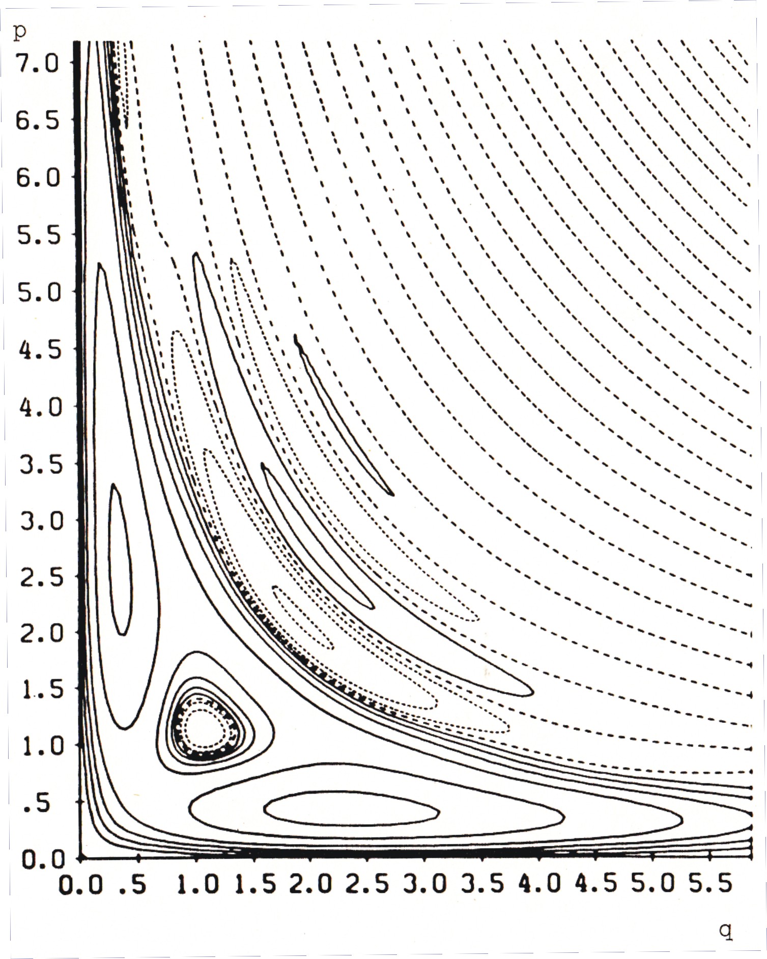
Figure 1: Contour curves in hartrees for the Wigner function for the beryllium atom. Reprinted with permission from Ref. [34].

Images for closed-shell atoms, based on Hartree–Fock configurations, are given in [34]. Experience with atomic ground-state Wigner functions allows one to reach the conclusion that the phase space region supporting an atomic Wigner quasidensity separates typically into three rough subregions. In the inner region the function $F_{1s}$ mostly takes positive values; but it may take negative values, due to complicated interplays among orbitals: the one-body Wigner distribution for the ground state of neon exhibited in [34] is a case in point, because of the weight of the $2p$ orbital. One sees that in the dominant middle region, this function takes large positive values; but negative values may also appear, due to entanglement between electron pairs. In both these regions the distribution barely oscillates. In the edge or “Airy” region we find an oscillatory decay regime. This decay of the Wigner distribution has been rigorously proved to be generic for systems with exponentially decaying (with linear exponents) states [61], such as those of atoms. As it turns out, the middle region corresponds to the region of the atom where the semiclassical approximation is reasonable; and the nodal curve by the frontier between the middle and the outer regions reproduces surprisingly well the border of the occupied region in the TF model of the atom – even for the $\mathrm{H}$-atom!

In the inner region the Wigner function definitely departs from the Thomas–Fermi Ansatz, in that it is always bounded; also, as soon as $N>2$, one finds “holes” of negative quasiprobability not far from the origin in phase space. In Figure 1 (taken from [34]) the hole produced by the interference of the $1s$ and $2s$ pairs is clearly visible.

On the strength of all this work we realize as well that WDFT provides an easily visualizable bridge between the TF and quantum approaches. We formalize this in Appendix A.

7 Natural Wigner orbitals

7.1 Preliminaries

Now we gear up for a new approach to $\mathcal{A}[d]$. Generally speaking, this is equivalent to looking for a functional $d_{2}[d]$, or for a functional $\rho_{2}[d]$ (one does not need $d_{2}$ to compute the Coulomb repulsion, its diagonal is enough); or even a functional $I[d]$, with $I$ the position intracule (for which we presume there is no representability problem), would be enough. In view of the Schmidt theorems on best approximation [50, 65], it is natural to use the spectral representation of $d(\mkern-1.0mu{\vec{\mkern 1.0muq}};\mkern-1.0mu{\vec{\mkern 1.0mup}};\varsigma;\varsigma^{\prime})$. Coleman’s representability theorems [4] can be construed as implying the natural expansion

$$d(\mkern-1.0mu{\vec{\mkern 1.0muq}};\mkern-1.0mu{\vec{\mkern 1.0mup}};\varsigma,\varsigma^{\prime})=\sum_{i=1}^{\infty}n_{i}\,f_{i}(\mkern-1.0mu{\vec{\mkern 1.0muq}};\mkern-1.0mu{\vec{\mkern 1.0mup}};\varsigma,\varsigma^{\prime}),$$

where the occupation numbers $n_{i}$ fulfil $0\leq n_{i}\leq 1$ and $\sum n_{i}=N$; we order them by descending size. A state with $n_{i}=0,1$ is a pinned, extremal or HF state; we already discussed them in subsection 2.1. Examples are known of interacting systems for which $0,1$ for some of the natural orbitals occur. For Coulomb systems typically the first $n_{i}$ for $1\leq i\leq N$ are close to $1$, corresponding to a state close to the best HF state; and the others are small. A proof of infinitude of non-zero occupation numbers in this context has been claimed in [66]. There are tantalizing cases, however, where the best numerical computations stubbornly yield reduced states of finite rank – see [67] for the first excited state of beryllium.

In the above sum, $i$ carries both spatial and spin indices. To have pure spin eigenstates, the non-diagonal spin blocks must be zero; moreover, in a spin-compensated, closed-shell situation the diagonal blocks are equal. Then $N$ must be even. In this case the spinless quasiprobability is of the form

$$d(\mkern-1.0mu{\vec{\mkern 1.0muq}};\mkern-1.0mu{\vec{\mkern 1.0mup}})=\sum_{i}\nu_{i}\,f_{i}(\mkern-1.0mu{\vec{\mkern 1.0muq}};\mkern-1.0mu{\vec{\mkern 1.0mup}}),$$

where the $f_{i}$ are still normalized to $1$, but now $0\leq\nu_{i}\leq 2$. Also, the $f_{i}$ verify

$$d\times f_{i}=f_{i}\times d=\nu_{i}f_{i}.$$ (36)

We call these $f_{i}$ the natural Wigner orbitals (NWO) – natural Wigner spatial orbitals would be more precise. We shall also need the natural Wigner spatial transitions, denoted $f_{ij}$. We know that in principle they can be found from the $f_{i}$ and, for $d$ spinless, they satisfy

$$d\times f_{ij}=\nu_{i}f_{ij};\qquad f_{ij}\times d=\nu_{j}f_{ij}.$$

7.2 The Müller functional

For $d$ a HF state, the general form of $\mathcal{A}[d]$ for an electronic interaction $f$ is well known:

$$\mathcal{A}[d] =\frac{1}{2}\biggl{[}\int\rho(\mkern-1.0mu{\vec{\mkern 1.0muq}}_{1})\rho(\mkern-1.0mu{\vec{\mkern 1.0muq}}_{2})f(\mkern-1.0mu{\vec{\mkern 1.0muq}}_{1},\mkern-1.0mu{\vec{\mkern 1.0muq}}_{2})\,d\mkern-1.0mu{\vec{\mkern 1.0muq}}_{1}\,d\mkern-1.0mu{\vec{\mkern 1.0muq}}_{2}-\int|\gamma(1,2)|^{2}\,f(\mkern-1.0mu{\vec{\mkern 1.0muq}}_{1},\mkern-1.0mu{\vec{\mkern 1.0muq}}_{2})\,d1\,d2\biggr{]}$$

$$=:D(\rho,\rho)-X(\gamma),$$ (37)

where $\rho$ and $\gamma$ are known functionals of $d$; the term $X(\gamma)$ is the exchange functional. If one uses (37) for arbitrary allowed quasidensities, one gets a functional for the interaction energy, proceeding through the pair density $\rho_{2}[d]$, denoted $\mathcal{A}^{\mathrm{HF}}$. Adding the kinetic and external energy functionals, we get a functional for the total energy, denoted $\mathcal{E}^{\mathrm{HF}}[d]$. Provided $f$ is positive semidefinite, its minimum is always reached in a HF state [52]. This means that $\mathcal{E}^{\mathrm{HF}}[d]$ renders an upper bound for the energy of the system; and that Slater determinants literally do no more than scratch the energy surface. The properties of $\mathcal{E}^{\mathrm{HF}}[d]$ are not very good, besides. Clearly it is not convex. Also, it does not respect a basic sum rule in general (this will be recalled in the next subsection). The difference between the minimum for the total energy attained by use of this expression and the “true” binding energy is generally called the correlation energy; it is obviously always negative.

The problem of finding $\rho_{2}[d]$ has been considered in the context of one-body density-matrix functional theory. In a remarkable paper Müller in 1984 [68] proposed an approximate formula for $D_{2}$ amounting, in our context, in the notation of (37), to the alternative functional:

$$\mathcal{A}^{\mathrm{M}}[d]=D(\rho,\rho)-X\bigl{(}\sqrt{\gamma}\,\bigr{)}.$$ (38)

Note that because of the equivalence of operator and Moyal product algebras, $\sqrt{\gamma}$ makes sense (meaning that $\sqrt{\gamma}\times\sqrt{\gamma}=\gamma$), provided one treads carefully. The concept is akin to Włodarz’s “phase space wave function” [21, 69].

After a period of some obscurity, the Müller functional was rediscovered [70, 71] and seems to be still in fashion [18]. The Müller functional is indeed convex [18]. Clearly $\mathcal{A}^{\mathrm{M}}[d]=\mathcal{A}^{\mathrm{HF}}[d]$ on the subset of extremal quasidensities. However, in general $\mathcal{A}^{\mathrm{M}}[d]\leq\mathcal{A}^{\mathrm{HF}}[d]$, and $\mathcal{A}^{\mathrm{M}}[d]$ actually tends to give lower bounds than the true values. To prove this in general would be important. It is only known for sure for $N=1,2$ as yet [18]; and, as perhaps could be expected, the proof in this last cited paper is quite complicated. We show within this section a much simplified proof by use of the exact functional, formulated in terms of NWOs.

7.3 General NWO functional theory

Let the spectral representation of $d$ be given, and denote

$$h_{i}=\int f_{i}(\mkern-1.0mu{\vec{\mkern 1.0muq}};\mkern-1.0mu{\vec{\mkern 1.0mup}};\varsigma,\varsigma^{\prime})\Bigl{(}\frac{p^{2}}{2}+V(\mkern-1.0mu{\vec{\mkern 1.0muq}}\,)\Bigr{)}\,d\mkern-1.0mu{\vec{\mkern 1.0muq}}\,d\mkern-1.0mu{\vec{\mkern 1.0mup}}\,d\varsigma\,d\varsigma^{\prime}.$$

The integrals are assumed to be finite. Then the energy is given by $\sum_{i}n_{i}h_{i}+V_{\mathrm{ee}}[d_{2}]$. We want to express the electron-electron repulsion $V_{\mathrm{ee}}[d_{2}]$ in the NWO representation. The expansion of $d_{2}$ in any orthonormal basis of eigentransitions, in particular the natural Wigner eigentransition basis, is denoted

$$d_{2}(1,2)=\sum_{ijkl}D^{ij}_{kl}\,f_{ki}(1)f_{lj}(2),$$

including spin indices. Note the symmetries

$$D^{ij}_{kl}={D^{kl}_{ij}}^{*},\quad D^{ij}_{kl}=-D^{ji}_{kl},\quad D^{ij}_{kl}=-D^{ij}_{lk},\quad D^{ij}_{kl}=D^{ji}_{lk}\,;$$ (39)

so one can rewrite the above expansion as

$$\sum_{i<j,\,k<l}D^{ij}_{kl}\bigl{(}f_{ki}(1)f_{lj}(2)+f_{lj}(1)f_{ki}(2)-f_{kj}(1)f_{li}(2)-f_{li}(1)f_{kj}(2)\bigr{)}.$$

Notice that in this language, the HF functional corresponds to taking, in the natural basis,

$$D^{ij}_{kl}=\frac{n_{i}n_{j}}{2}(\delta^{i}_{k}\,\delta^{j}_{l}-\delta^{i}_{l}\,\delta^{j}_{k}).$$

In principle $d_{2}$ has sixteen spin blocks, but, as a consequence of requiring pure spin states, only six differ from zero:

$${d_{2}}^{{\mathord{\uparrow}}{\mathord{\uparrow}}}_{{\mathord{\uparrow}}{\mathord{\uparrow}}},\quad{d_{2}}^{{\mathord{\downarrow}}{\mathord{\downarrow}}}_{{\mathord{\downarrow}}{\mathord{\downarrow}}},\quad{d_{2}}^{{\mathord{\uparrow}}{\mathord{\downarrow}}}_{{\mathord{\uparrow}}{\mathord{\downarrow}}},\quad{d_{2}}^{{\mathord{\downarrow}}{\mathord{\uparrow}}}_{{\mathord{\downarrow}}{\mathord{\uparrow}}},\quad{d_{2}}^{{\mathord{\uparrow}}{\mathord{\downarrow}}}_{{\mathord{\downarrow}}{\mathord{\uparrow}}},\quad{d_{2}}^{{\mathord{\downarrow}}{\mathord{\uparrow}}}_{{\mathord{\uparrow}}{\mathord{\downarrow}}},$$

and only three of those are independent. With this notation, $V_{\mathrm{ee}}[d_{2}]$ is given by

$$\sum_{pqrt}\langle rt\mathbin{|}pq\rangle\bigl{(}D^{p{\mathord{\uparrow}},q{\mathord{\uparrow}}}_{r{\mathord{\uparrow}},t{\mathord{\uparrow}}}+D^{p{\mathord{\uparrow}},q{\mathord{\downarrow}}}_{r{\mathord{\uparrow}},t{\mathord{\downarrow}}}+D^{p{\mathord{\downarrow}},q{\mathord{\uparrow}}}_{r{\mathord{\downarrow}},t{\mathord{\uparrow}}}+D^{p{\mathord{\downarrow}},q{\mathord{\downarrow}}}_{r{\mathord{\downarrow}},t{\mathord{\downarrow}}}\bigr{)},$$

where

$$\langle rt\mathbin{|}pq\rangle:=\int\frac{f_{pr}(\mkern-1.0mu{\vec{\mkern 1.0muq}}_{1},\mkern-1.0mu{\vec{\mkern 1.0mup}}_{1})f_{qt}(\mkern-1.0mu{\vec{\mkern 1.0muq}}_{2},\mkern-1.0mu{\vec{\mkern 1.0mup}}_{2})}{|\mkern-1.0mu{\vec{\mkern 1.0muq}}_{1}-\mkern-1.0mu{\vec{\mkern 1.0muq}}_{2}|}\,d\mkern-1.0mu{\vec{\mkern 1.0muq}}_{1}\,d\mkern-1.0mu{\vec{\mkern 1.0muq}}_{2}\,d\mkern-1.0mu{\vec{\mkern 1.0mup}}_{1}\,d\mkern-1.0mu{\vec{\mkern 1.0mup}}_{2},$$

with purely spatial indices. Note that the other two nonzero blocks cannot contribute to this Coulomb integral. At this point, it is convenient to introduce spinless density matrices by tracing:

$$\nu_{p}=n_{p{\mathord{\uparrow}}}+n_{p{\mathord{\downarrow}}},\qquad\widetilde{D}^{pq}_{rt}:=D^{p{\mathord{\uparrow}},q{\mathord{\uparrow}}}_{r{\mathord{\uparrow}},t{\mathord{\uparrow}}}+D^{p{\mathord{\uparrow}},q{\mathord{\downarrow}}}_{r{\mathord{\uparrow}},t{\mathord{\downarrow}}}+D^{p{\mathord{\downarrow}},q{\mathord{\uparrow}}}_{r{\mathord{\downarrow}},t{\mathord{\uparrow}}}+D^{p{\mathord{\downarrow}},q{\mathord{\downarrow}}}_{r{\mathord{\downarrow}},t{\mathord{\downarrow}}},$$ (40)

and write

$$E=\sum_{p}\nu_{p}h_{p}+\sum_{pqrt}\widetilde{D}^{pq}_{rt}\langle rt\mathbin{|}pq\rangle.$$

Note now that the sums:

$$\int d_{2}(1,2)\,d1\,d2=\sum_{ijkl}D^{ij}_{kl}\int f_{ki}(1)f_{lj}(2)\,d1\,d2=\sum_{ijkl}D^{ij}_{kl}\,\delta_{i}^{k}\delta_{j}^{l}=\sum_{ij}D^{ij}_{ij}$$

must be $N(N-1)/2$, the number of electron pairs, while

$$\sum_{ijkl}\frac{n_{i}n_{j}}{2}(\delta^{i}_{k}\delta^{j}_{l}-\delta^{i}_{l}\delta^{j}_{k}\delta_{i}^{k}\delta_{j}^{l})=\frac{N^{2}}{2}-\frac{\sum n_{i}^{2}}{2}>\frac{N(N-1)}{2},$$

unless all $n_{i}$ are $0$ or $1$, that is, the pure HF case. This is the sum rule we alluded to in the previous subsection. Let us baptize our ignorance

$$\Gamma^{ij}_{kl}:=D^{ij}_{kl}-\frac{n_{i}n_{j}}{2}(\delta^{i}_{k}\delta^{j}_{l}-\delta^{i}_{l}\delta^{j}_{k});$$

this cumulant deserves perhaps to be called the correlation matrix. We now observe that, while certainly $\int\rho(1)\rho(2)\,d1\,d2=O(N^{2})$, we have

$$\sum_{ijkl}\int\Gamma^{ij}_{kl}f_{ki}(1)f_{lj}(2)\,d1\,d2=\sum_{i}\frac{n_{i}^{2}-n_{i}}{2}=O(N).$$ (41)

This kind of observation is useful in Thomas–Fermi theory.

7.4 NWO for ground states of two-electron systems

For two-electron atoms we can do much better. Let us invoke invariance of the Hamiltonian under time inversion – the latter is represented by an antiunitary operator related to spinor conjugation that we need not write out. This assumption is not essential, but simplifies matters, and moreover holds in most cases of interest; it entails that the eigenstate wave functions are real. It is most instructive to start from a general basis of eigentransitions and construct the natural basis out of it. This is equivalent to recasting the results of the classic work [75] in our language.

So let an orthonormal basis $\{f_{nm}\}$ for single-body functions on phase space be given, arbitrary except for the properties of Theorem 1. Consider singlet states. We want to expand a normalized singlet 2-Wigner function $P_{2}\equiv d_{2}$ in terms of the $f_{nm}$. Its spatial part must be symmetric under exchange of coordinates; thus $P_{2}$ is of the form

$$P_{2}(\mkern-1.0mu{\vec{\mkern 1.0muq}}_{1},\mkern-1.0mu{\vec{\mkern 1.0muq}}_{2};\mkern-1.0mu{\vec{\mkern 1.0mup}}_{1},\mkern-1.0mu{\vec{\mkern 1.0mup}}_{2};\varsigma_{1},\varsigma_{2},\varsigma^{\prime}_{1},\varsigma^{\prime}_{2})=\frac{1}{2}({\mathord{\uparrow}}_{1}{\mathord{\downarrow}}_{2}-{\mathord{\downarrow}}_{1}{\mathord{\uparrow}}_{2})({\mathord{\uparrow}}_{1^{\prime}}{\mathord{\downarrow}}_{2^{\prime}}-{\mathord{\downarrow}}_{1^{\prime}}{\mathord{\uparrow}}_{2^{\prime}})f(\mkern-1.0mu{\vec{\mkern 1.0muq}}_{1},\mkern-1.0mu{\vec{\mkern 1.0muq}}_{2};\mkern-1.0mu{\vec{\mkern 1.0mup}}_{1},\mkern-1.0mu{\vec{\mkern 1.0mup}}_{2}),$$ (42)

where

$$f(\mkern-1.0mu{\vec{\mkern 1.0muq}}_{1},\mkern-1.0mu{\vec{\mkern 1.0muq}}_{2};\mkern-1.0mu{\vec{\mkern 1.0mup}}_{1},\mkern-1.0mu{\vec{\mkern 1.0mup}}_{2})=\frac{1}{4}\sum_{klmr}C_{mr}C_{kl} \bigl{[}f_{mk}(\mkern-1.0mu{\vec{\mkern 1.0muq}}_{1};\mkern-1.0mu{\vec{\mkern 1.0mup}}_{1})f_{rl}(\mkern-1.0mu{\vec{\mkern 1.0muq}}_{2};\mkern-1.0mu{\vec{\mkern 1.0mup}}_{2})+f_{rl}(\mkern-1.0mu{\vec{\mkern 1.0muq}}_{1};\mkern-1.0mu{\vec{\mkern 1.0mup}}_{1})f_{mk}(\mkern-1.0mu{\vec{\mkern 1.0muq}}_{2};\mkern-1.0mu{\vec{\mkern 1.0mup}}_{2})$$

$$\quad+f_{ml}(\mkern-1.0mu{\vec{\mkern 1.0muq}}_{1};\mkern-1.0mu{\vec{\mkern 1.0mup}}_{1})f_{rk}(\mkern-1.0mu{\vec{\mkern 1.0muq}}_{2};\mkern-1.0mu{\vec{\mkern 1.0mup}}_{2})+f_{rk}(\mkern-1.0mu{\vec{\mkern 1.0muq}}_{1};\mkern-1.0mu{\vec{\mkern 1.0mup}}_{1})f_{ml}(\mkern-1.0mu{\vec{\mkern 1.0muq}}_{2};\mkern-1.0mu{\vec{\mkern 1.0mup}}_{2})\bigr{]},$$ (43)

with $C_{kl}=C_{lk}$ real and $\sum_{kl}C_{kl}^{2}=1$. Each group of terms is real in view of $\overline{f_{mk}}=f_{km}$ and the normalization ensures that

$$\int P_{2}(\mkern-1.0mu{\vec{\mkern 1.0muq}}_{1},\mkern-1.0mu{\vec{\mkern 1.0muq}}_{2};\mkern-1.0mu{\vec{\mkern 1.0mup}}_{1},\mkern-1.0mu{\vec{\mkern 1.0mup}}_{2};\varsigma_{1},\varsigma_{2},\varsigma_{1},\varsigma_{2})\,d\mkern-1.0mu{\vec{\mkern 1.0muq}}_{1}\,d\mkern-1.0mu{\vec{\mkern 1.0muq}}_{2}\,d\mkern-1.0mu{\vec{\mkern 1.0mup}}_{1}\,d\mkern-1.0mu{\vec{\mkern 1.0mup}}_{2}\,d\varsigma_{1}\,d\varsigma_{2}=1$$

in (42). It is clear that in the singlet case ${d_{2}}^{{\mathord{\uparrow}}{\mathord{\uparrow}}}_{{\mathord{\uparrow}}{\mathord{\uparrow}}}={d_{2}}^{{\mathord{\downarrow}}{\mathord{\downarrow}}}_{{\mathord{\downarrow}}{\mathord{\downarrow}}}=0$ and that ${d_{2}}^{{\mathord{\uparrow}}{\mathord{\downarrow}}}_{{\mathord{\uparrow}}{\mathord{\downarrow}}}={d_{2}}^{{\mathord{\downarrow}}{\mathord{\uparrow}}}_{{\mathord{\downarrow}}{\mathord{\uparrow}}}=\tfrac{1}{2}f$.

The corresponding 1-Wigner distribution is obtained at once by integration,

$$d(\mkern-1.0mu{\vec{\mkern 1.0muq}};\mkern-1.0mu{\vec{\mkern 1.0mup}};\varsigma,\varsigma^{\prime})=({\mathord{\uparrow}}{\mathord{\uparrow}}^{\prime}+{\mathord{\downarrow}}{\mathord{\downarrow}}^{\prime})\sum_{km}\gamma_{mk}f_{mk}(\mkern-1.0mu{\vec{\mkern 1.0muq}};\mkern-1.0mu{\vec{\mkern 1.0mup}})=\begin{pmatrix}\sum_{km}\gamma_{mk}f_{mk}(\mkern-1.0mu{\vec{\mkern 1.0muq}};\mkern-1.0mu{\vec{\mkern 1.0mup}})&0\\[3.0pt] 0&\sum_{km}\gamma_{mk}f_{mk}(\mkern-1.0mu{\vec{\mkern 1.0muq}};\mkern-1.0mu{\vec{\mkern 1.0mup}})\end{pmatrix},$$

where $\gamma:=[\gamma_{mk}]=\bigl{[}\sum_{l}C_{ml}C_{kl}\bigr{]}$ is a symmetric (and positive semidefinite) matrix. The matrix $C$ determines a real quadratic form that can be made diagonal by an orthogonal change of basis $O=[O_{lm}]$,

$$C=O\,c\,O^{t},\quad\mbox{implying}\quad\gamma=O\,c^{2}\,O^{t},$$

where $c=[c_{r}\,\delta_{rs}]$. These elements $c_{r}$ are real, but note that some of them may be negative. Let us now make the definition:

$$\chi_{rp}:=\sum_{mk}O_{mr}f_{mk}O_{kp},\quad\mbox{so that}\quad f_{km}=\sum_{rp}O_{kp}\chi_{pr}O_{mr}.$$

The diagonal $\chi_{rr}\equiv\chi_{r}$ are real: $\overline{\chi_{r}}=\sum_{mk}O_{mr}f_{km}O_{kr}=\chi_{r}$, and more generally $\overline{\chi_{rs}}=\chi_{sr}$; and it is easy to check that

$$\chi_{i}\times\chi_{j}=\sum_{mk}O_{mi}f_{mk}O_{ki}\times\sum_{ls}O_{lj}f_{ls}O_{sj}=\sum_{ms}O_{mi}f_{ms}O_{sj}\,\delta_{ij}=\chi_{i}\,\delta_{ij},$$

and that, with $d_{*}$ denoting either of the two nonvanishing spin components of $d$,

$$d_{*}=\sum_{km}\gamma_{mk}f_{mk}=\sum_{rp}\sum_{km}O_{mr}\gamma_{mk}O_{kp}\,\chi_{pr}=\sum_{rp}c^{2}_{r}\,\delta_{rp}\chi_{pr}=:\sum_{r}n_{r}\chi_{r}$$

(on writing $n_{r}:=c_{r}^{2}$), so the $\chi_{i}$ solve the simultaneous equations

$$d_{*}\times\chi_{i}=\chi_{i}\times d_{*}=n_{i}\chi_{i},$$

which is (36) up to a factor. Furthermore, $\sum n_{i}=\operatorname{tr}(c^{2})=\operatorname{tr}(C^{2})=1$. The $n_{i}$ are the “occupation numbers” for “natural Wigner orbitals” $\chi_{i}$; we have recovered the Coleman results in this case. It remains to compute

$$\sum_{kl,mr}C_{mr}C_{kl}\,f_{mk}(\mkern-1.0mu{\vec{\mkern 1.0muq}}_{1};\mkern-1.0mu{\vec{\mkern 1.0mup}}_{1})f_{rl}(\mkern-1.0mu{\vec{\mkern 1.0muq}}_{2};\mkern-1.0mu{\vec{\mkern 1.0mup}}_{2}) =\sum_{vt,klmr}c_{v}c_{t}O_{mv}O_{rv}O_{kt}O_{lt}\,f_{mk}(\mkern-1.0mu{\vec{\mkern 1.0muq}}_{1};\mkern-1.0mu{\vec{\mkern 1.0mup}}_{1})f_{rl}(\mkern-1.0mu{\vec{\mkern 1.0muq}}_{2};\mkern-1.0mu{\vec{\mkern 1.0mup}}_{2})$$

$$=\sum_{vt}c_{v}c_{t}\,\chi_{vt}(\mkern-1.0mu{\vec{\mkern 1.0muq}}_{1};\mkern-1.0mu{\vec{\mkern 1.0mup}}_{1})\chi_{vt}(\mkern-1.0mu{\vec{\mkern 1.0muq}}_{2};\mkern-1.0mu{\vec{\mkern 1.0mup}}_{2}),$$

and similarly for the other terms in (43).

As $c_{r}=\pm\sqrt{n_{r}}$, in order to obtain $d_{2}[d]$ and thus $\mathcal{A}[d]$ one needs “only” to determine an infinite number of signs. Recall that in (40), in view of (42), the terms $D^{p{\mathord{\uparrow}},q{\mathord{\uparrow}}}_{r{\mathord{\uparrow}},t{\mathord{\uparrow}}}$ and $D^{p{\mathord{\downarrow}},q{\mathord{\downarrow}}}_{r{\mathord{\downarrow}},t{\mathord{\downarrow}}}$ vanish. We see that $\widetilde{D}^{pq}_{rt}=c_{r}c_{p}\,\delta_{rt}\,\delta^{pq}$ in the new basis. We use the notations

$$\chi_{pr}(\mkern-1.0mu{\vec{\mkern 1.0muq}}):=\int\chi_{pr}(\mkern-1.0mu{\vec{\mkern 1.0muq}},\mkern-1.0mu{\vec{\mkern 1.0mup}})\,d\mkern-1.0mu{\vec{\mkern 1.0mup}},\qquad L_{rp}:=\langle rr\mathbin{|}pp\rangle=\int\frac{\chi_{pr}(\mkern-1.0mu{\vec{\mkern 1.0muq}}_{1})\chi_{pr}(\mkern-1.0mu{\vec{\mkern 1.0muq}}_{2})}{|\mkern-1.0mu{\vec{\mkern 1.0muq}}_{1}-\mkern-1.0mu{\vec{\mkern 1.0muq}}_{2}|}\,d\mkern-1.0mu{\vec{\mkern 1.0muq}}_{1}\,d\mkern-1.0mu{\vec{\mkern 1.0muq}}_{2},$$ (44)

borrowing now the eigentransitions $\chi_{pr}$ in the expansion of $d_{2}$. Note that these terms arise from correlation between electrons with opposite spin. They are real: in view of (4), the integrals over the momenta yield real functions since the corresponding wave functions are real. In particular $\chi_{pr}(\mkern-1.0mu{\vec{\mkern 1.0muq}})=\chi_{rp}(\mkern-1.0mu{\vec{\mkern 1.0muq}})$, and $L_{rp}=L_{pr}$, too. In the weak correlation regime, when there is a dominant state close to the best HF state, Löwdin and Shull [75, 76] empirically found long ago that, if conventionally $c_{1}$ was taken equal to $+\sqrt{n_{1}}$, then (most of) the other signs were negative. This gives rise to:

$$d_{2\mathrm{L}}(1,2) =\text{(spin factor) }\times\biggl{[}n_{1}\chi_{1}(\mkern-1.0mu{\vec{\mkern 1.0muq}}_{1})\chi_{1}(\mkern-1.0mu{\vec{\mkern 1.0muq}}_{2})-\sum_{p\geq 2}\sqrt{n_{1}n_{p}}\bigl{(}\chi_{p1}(\mkern-1.0mu{\vec{\mkern 1.0muq}}_{1})\chi_{p1}(\mkern-1.0mu{\vec{\mkern 1.0muq}}_{2})+\chi_{1p}(\mkern-1.0mu{\vec{\mkern 1.0muq}}_{1})\chi_{1p}(\mkern-1.0mu{\vec{\mkern 1.0muq}}_{2})\bigr{)}$$

$$\qquad+\sum_{p,r\geq 2}\sqrt{n_{r}n_{p}}\,\chi_{rp}(\mkern-1.0mu{\vec{\mkern 1.0muq}}_{1})\chi_{rp}(\mkern-1.0mu{\vec{\mkern 1.0muq}}_{2})\biggr{]},$$ (45)

$$\mathcal{A}^{\mathrm{L}}[d] :=n_{1}L_{11}-2\sum_{p\geq 2}\sqrt{n_{1}n_{p}}\,L_{1p}+\sum_{p,r\geq 2}\sqrt{n_{r}n_{p}}\,L_{rp}.$$ (46)

In this connection the work of Kutzelnigg [77] was decisive as well. As mentioned before, the natural orbital construction guarantees term-by-term the most rapid approximation to $d_{2}$. The case where the sum stops merely at $p=2$ accounts with remarkable accuracy for a good fraction of the radial correlation energy [75]. We might call these the Shull–Löwdin–Kutzelnigg functionals (SLK functionals, for short). For the comparison with the Müller functional in the next subsection, the configuration of signs turns out to be irrelevant, and generally we call the analogue of (46) with any sign choice a SLK functional.

The case for the (strict) SLK functional has been argued for mathematically as follows. By the Rayleigh principle, the quadratic form representing the energy has a minimum eigenvalue when $(c_{1}\ c_{2}\ \cdots)^{t}$ is an eigenvector, that is,

$$E_{0}\begin{pmatrix}c_{1}\\ c_{2}\\ \vdots\end{pmatrix}=\begin{pmatrix}2n_{1}h_{1}+L_{11}&L_{12}&\cdots\\ L_{12}&2n_{2}h_{2}+L_{22}&\cdots\\ \vdots&\vdots&\ddots\end{pmatrix}\begin{pmatrix}c_{1}\\ c_{2}\\ \vdots\end{pmatrix}.$$

Therefore, for all $r$:

$$E_{0}=2n_{r}h_{r}+L_{rr}+\sum_{p\neq r}L_{rp}\,\frac{c_{p}}{c_{r}}.$$

Only the two-body part of the Hamiltonian contributes to the off-diagonal terms. Well-known properties of the Coulomb potential ensure that these are all positive. Indeed, the Coulomb potential is positive definite in that its Fourier transform is a positive distribution. Or one can use its integral representation [78, Chap. 5]:

$$\frac{\pi^{3}}{|\mkern-1.0mu{\vec{\mkern 1.0muq}}_{1}-\mkern-1.0mu{\vec{\mkern 1.0muq}}_{2}|}=\int\frac{1}{|\vec{z}-\mkern-1.0mu{\vec{\mkern 1.0muq}}_{1}|}\frac{1}{|\vec{z}-\mkern-1.0mu{\vec{\mkern 1.0muq}}_{2}|}\,d^{3}z.$$

Thus, whenever $n_{1}$ (that is to say $c_{1}$) is dominant, to minimize $E_{0}$ we must put $c_{2}$ negative, and probably $c_{3},c_{4},\dots$ as well. We remark that in the weak correlation regime the energy matrix is diagonally dominant, and diagonalization of the quadratic form proceeds without obstacle; all pivots will be negative. Diagonal dominance ensures that the energy matrix is negative definite [79] as well. Nevertheless, while this reasoning shows that there must be some negative signs, it does not prove that all signs beyond that of $c_{1}$ are negative.

A different argument to the same effect was put forward in [80]. We summarize it next. Consider the gradient of the energy,

$$\frac{\partial E}{\partial c_{r}}=4h_{r}c_{r}+2\sum_{p}c_{p}L_{rp}-2c_{r}\lambda,$$

where $\lambda$ is a Lagrange multiplier, at the “Hartree–Fock point”, defined by $c_{1}=1$, $c_{2}=c_{3}=\cdots=0$. For $r>1$ only the second term on the right hand side contributes. Thus the only way to obtain a negative gradient is for $c_{r}$ to become negative in the minimization process. Also in [80] it is remarked that for the negative hydrogen ion $\mathrm{H}^{-}$, wherein the largest occupation number differs significantly from $1$, the sign rule numerically holds true. Again, the argument is persuasive, but not conclusive, since a moment’s reflection shows that it refers to the approximation from HF states rather than to the exact state.

We now list some properties and traits of the SLK functional for singlet states.

1. The sum rule $\int\rho_{2\mathrm{L}}(1,2)\,d1\,d2:=\int d_{2\mathrm{L}}(\mkern-1.0mu{\vec{\mkern 1.0muq}}_{1},\mkern-1.0mu{\vec{\mkern 1.0muq}}_{2};\mkern-1.0mu{\vec{\mkern 1.0mup}}_{1},\mkern-1.0mu{\vec{\mkern 1.0mup}}_{2})\,d\mkern-1.0mu{\vec{\mkern 1.0muq}}_{1}\,d\mkern-1.0mu{\vec{\mkern 1.0mup}}_{1}\,d\mkern-1.0mu{\vec{\mkern 1.0muq}}_{2}\,d\mkern-1.0mu{\vec{\mkern 1.0mup}}_{2}=1$ is (of course) fulfilled.

2. The pair coincidence probability is a perfect square for any rank (and actually any choice of signs).

3. For pinned states, it reproduces the results of the HF functional.

4. The correlation energy is negative.

5. The SLK functional scales linearly:

   $$\mathcal{A}[d_{\lambda}]=\lambda\,\mathcal{A}[d],$$

   with $d_{\lambda}$ as in subsection 3.1. So the correlation energy functional must scale linearly, too.

6. The SLK functional satisfies known constraints from the $D_{2}$-representability theory [4].

The previous one is a typical closed-shell configuration, and for such both spin components are completely identical. However, the fact of the matter is that occupation numbers always are evenly degenerate for any two-electron state [4].

7.5 Shull–Löwdin–Kutzelnigg versus Müller

Let us write the Müller functional (38) in terms of NW orbitals:

$$\rho_{2\mathrm{M}}(\mkern-1.0mu{\vec{\mkern 1.0muq}}_{1},\mkern-1.0mu{\vec{\mkern 1.0muq}}_{2}):=\frac{1}{2}\sum_{jk}n_{j}n_{k}\chi_{j}(\mkern-1.0mu{\vec{\mkern 1.0muq}}_{1})\chi_{k}(\mkern-1.0mu{\vec{\mkern 1.0muq}}_{2})-\frac{1}{2}\sum_{jk}\sqrt{n_{j}n_{k}}\,\chi_{jk}(\mkern-1.0mu{\vec{\mkern 1.0muq}}_{1})\chi_{kj}(\mkern-1.0mu{\vec{\mkern 1.0muq}}_{2}).$$

The integral over all coordinates comes out right as 1 (see below). But clearly $d_{2\mathrm{M}}$ does not possess the antisymmetry properties required in (39). As recognized in the original article [68], the corresponding pair density $\rho_{2\mathrm{M}}(\mkern-1.0mu{\vec{\mkern 1.0muq}},\mkern-1.0mu{\vec{\mkern 1.0muq}})$ can take negative values for some states. Thus it is not surprising that the Müller functional tends to give lower bounds than the true values; when applied formally to the hydrogen atom, this is the case. Unphysical probabilities together with the overbinding property clearly indicate that it does not correspond to physically realizable states.

Reference [18] amounts to a long analysis of the Müller functional, crowned by a proof that it gives lower energy values than the true values for helium. Now we deliver the promised simpler (as well as more informative) proof of that theorem.

Theorem 6.

For the isoelectronic helium-like series, the Müller functional $\mathcal{A}^{\mathrm{M}}[d]$ is a lower bound to quantum mechanics.

Proof.

We simply compare directly the Müller and SLK functionals. In the notation of (44), with $\rho_{i}(\mkern-1.0mu{\vec{\mkern 1.0muq}})=\int\chi_{i}(\mkern-1.0mu{\vec{\mkern 1.0muq}},\mkern-1.0mu{\vec{\mkern 1.0mup}})\,d\mkern-1.0mu{\vec{\mkern 1.0mup}}$ too, the pair density coming from the SLK functional is

$$\rho_{2\mathrm{L}}(\mkern-1.0mu{\vec{\mkern 1.0muq}}_{1},\mkern-1.0mu{\vec{\mkern 1.0muq}}_{2})=\sum_{i}n_{i}\rho_{i}(\mkern-1.0mu{\vec{\mkern 1.0muq}}_{1})\rho_{i}(\mkern-1.0mu{\vec{\mkern 1.0muq}}_{2})-2\sum_{j\geq 2}\sqrt{n_{1}n_{j}}\,\chi_{1j}(\mkern-1.0mu{\vec{\mkern 1.0muq}}_{1})\chi_{1j}(\mkern-1.0mu{\vec{\mkern 1.0muq}}_{2})+\!\sum_{i,j\geq 2,\,i\neq j}\!\sqrt{n_{i}n_{j}}\,\chi_{ij}(\mkern-1.0mu{\vec{\mkern 1.0muq}}_{1})\chi_{ij}(\mkern-1.0mu{\vec{\mkern 1.0muq}}_{2}),$$

$$\quad\mbox{normalized by}\quad\int\rho_{2\mathrm{L}}(\mkern-1.0mu{\vec{\mkern 1.0muq}}_{1},\mkern-1.0mu{\vec{\mkern 1.0muq}}_{2})\,d\mkern-1.0mu{\vec{\mkern 1.0muq}}_{1}\,d\mkern-1.0mu{\vec{\mkern 1.0muq}}_{2}=\sum_{i}n_{i}=1.$$ (47)

For the same object in our (two-electron, closed-shell) context, the Müller functional gives

$$\rho_{2\mathrm{M}}(\mkern-1.0mu{\vec{\mkern 1.0muq}}_{1},\mkern-1.0mu{\vec{\mkern 1.0muq}}_{2})=\frac{1}{2}\rho(\mkern-1.0mu{\vec{\mkern 1.0muq}}_{1})\rho(\mkern-1.0mu{\vec{\mkern 1.0muq}}_{2})-\sum_{i}n_{i}\rho_{i}(\mkern-1.0mu{\vec{\mkern 1.0muq}}_{1})\rho_{i}(\mkern-1.0mu{\vec{\mkern 1.0muq}}_{2})-\sum_{i\neq j}\sqrt{n_{i}n_{j}}\,\chi_{ij}(\mkern-1.0mu{\vec{\mkern 1.0muq}}_{1})\chi_{ij}(\mkern-1.0mu{\vec{\mkern 1.0muq}}_{2}).$$ (48)

It is perhaps not obvious which of the contributions $\tfrac{1}{2}\rho(\mkern-1.0mu{\vec{\mkern 1.0muq}}_{1})\rho(\mkern-1.0mu{\vec{\mkern 1.0muq}}_{2})$ or $2\sum_{i}n_{i}\rho_{i}(\mkern-1.0mu{\vec{\mkern 1.0muq}}_{1})\rho_{i}(\mkern-1.0mu{\vec{\mkern 1.0muq}}_{2})$ will be larger. However, on using $n_{i}^{2}=n_{i}-\sum_{j\neq i}n_{i}n_{j}$, we compute the “defect”:

$$2\sum_{i}n_{i}\rho_{i}(\mkern-1.0mu{\vec{\mkern 1.0muq}}_{1})\rho_{i}(\mkern-1.0mu{\vec{\mkern 1.0muq}}_{2})-\frac{1}{2}\rho(\mkern-1.0mu{\vec{\mkern 1.0muq}}_{1})\rho(\mkern-1.0mu{\vec{\mkern 1.0muq}}_{2}) =2\sum_{i}n_{i}\rho_{i}(\mkern-1.0mu{\vec{\mkern 1.0muq}}_{1})\rho_{i}(\mkern-1.0mu{\vec{\mkern 1.0muq}}_{2})-2\Bigl{(}\sum_{i}n_{i}\rho_{i}(\mkern-1.0mu{\vec{\mkern 1.0muq}}_{1})\Bigr{)}\Bigl{(}\sum_{j}n_{j}\rho_{j}(\mkern-1.0mu{\vec{\mkern 1.0muq}}_{2})\Bigr{)}$$

$$=\sum_{j\neq i}n_{i}n_{j}\bigl{(}\rho_{i}(\mkern-1.0mu{\vec{\mkern 1.0muq}}_{1})-\rho_{j}(\mkern-1.0mu{\vec{\mkern 1.0muq}}_{1})\bigr{)}\bigl{(}\rho_{i}(\mkern-1.0mu{\vec{\mkern 1.0muq}}_{2})-\rho_{j}(\mkern-1.0mu{\vec{\mkern 1.0muq}}_{2})\bigr{)}.$$

This must still be integrated with $1/{|\mkern-1.0mu{\vec{\mkern 1.0muq}}_{1}-\mkern-1.0mu{\vec{\mkern 1.0muq}}_{2}|}$; then we see that the positivity of the Coulomb potential alluded to in the previous subsection does the job, establishing that $\mathcal{A}^{\mathrm{M}}[d]<\mathcal{A}^{\mathrm{L}}[d]$. ∎

Remark 1

For a chemists’ chemist, the proof is surely over. A mathematically minded one, however, would argue that we still ought to provide for convergence of the series representing the difference in energy. To guarantee that, consider the expression

$$S=\sum_{j\neq i}n_{i}n_{j}\int\frac{F_{ij}(\mkern-1.0mu{\vec{\mkern 1.0muq}}_{1})F_{ij}(\mkern-1.0mu{\vec{\mkern 1.0muq}}_{2})}{|\mkern-1.0mu{\vec{\mkern 1.0muq}}_{1}-\mkern-1.0mu{\vec{\mkern 1.0muq}}_{2}|}\,d\mkern-1.0mu{\vec{\mkern 1.0muq}}_{1}\,d\mkern-1.0mu{\vec{\mkern 1.0muq}}_{2},$$ (49)

where $F_{ij}:=\rho_{i}-\rho_{j}$. The Hardy–Littlewood–Sobolev inequality [81, Sect. 2.3] gives, for a suitable (sharp) constant $C_{1}$, the bound

$$S \leq C_{1}\sum_{j\neq i}n_{i}n_{j}\,\|F_{ij}\|^{2}_{6/5}=C_{1}\sum_{j\neq i}n_{i}n_{j}\,\|\rho_{i}-\rho_{j}\|^{2}_{6/5}$$

$$\leq 2C_{1}\sum_{i,j\geq 1}n_{i}n_{j}\bigl{(}\|\rho_{i}\|^{2}_{6/5}+\|\rho_{j}\|^{2}_{6/5}\bigr{)}=4C_{1}\sum_{i\geq 1}n_{i}\|\rho_{i}\|^{2}_{6/5}.$$

As a marginal of a Wigner function, each $\rho_{i}$ is positive and lies in $L^{1}(\mathbb{R}^{3})$, with $\|\rho_{i}\|=1$. However, we need to confirm that each $\rho_{i}(\mkern-1.0mu{\vec{\mkern 1.0muq}})$ belongs to $L^{6/5}(\mathbb{R}^{3})$. Finiteness of the kinetic energy produces the estimate we need for that. As suggested already by Moyal [12], from formula (3) for (spinless) momentum states we obtain:

$$\infty>\int\frac{p^{2}}{2}f(\mkern-1.0mu{\vec{\mkern 1.0muq}};\mkern-1.0mu{\vec{\mkern 1.0mup}})\,d\mkern-1.0mu{\vec{\mkern 1.0muq}}\,d\mkern-1.0mu{\vec{\mkern 1.0mup}} =\frac{1}{2\pi^{3}}\int p^{2}\gamma(\mkern-1.0mu{\vec{\mkern 1.0mup}}^{\prime};\mkern-1.0mu{\vec{\mkern 1.0mup}}^{\prime\prime})e^{i(\mkern-1.0mu{\vec{\mkern 1.0muq}}\cdot(\mkern-1.0mu{\vec{\mkern 1.0mup}}^{\prime}-\mkern-1.0mu{\vec{\mkern 1.0mup}}^{\prime\prime}))}\,\delta\bigl{(}\mkern-1.0mu{\vec{\mkern 1.0mup}}-\tfrac{1}{2}(\mkern-1.0mu{\vec{\mkern 1.0mup}}^{\prime}+\mkern-1.0mu{\vec{\mkern 1.0mup}}^{\prime\prime})\bigr{)}\,d\mkern-1.0mu{\vec{\mkern 1.0muq}}\,d\mkern-1.0mu{\vec{\mkern 1.0mup}}\,d\mkern-1.0mu{\vec{\mkern 1.0mup}}^{\prime}\,d\mkern-1.0mu{\vec{\mkern 1.0mup}}^{\prime\prime}$$

$$=-\frac{1}{8}\int\bigl{(}\nabla_{\mkern-1.0mu{\vec{\mkern 1.0mux}}}-\nabla_{\mkern-1.0mu{\vec{\mkern 1.0mux}}^{\prime}}\bigr{)}^{2}\gamma(\mkern-1.0mu{\vec{\mkern 1.0mux}};\mkern-1.0mu{\vec{\mkern 1.0mux}}^{\prime})\bigr{|}_{\mkern-1.0mu{\vec{\mkern 1.0mux}}=\mkern-1.0mu{\vec{\mkern 1.0mux}}^{\prime}=\mkern-1.0mu{\vec{\mkern 1.0muq}}}\ d\mkern-1.0mu{\vec{\mkern 1.0muq}}.$$

On account of the natural orbital expansion $\gamma(\mkern-1.0mu{\vec{\mkern 1.0mux}};\mkern-1.0mu{\vec{\mkern 1.0mux}}^{\prime})=\sum_{i}n_{i}\phi_{i}(\mkern-1.0mu{\vec{\mkern 1.0mux}})\phi_{i}(\mkern-1.0mu{\vec{\mkern 1.0mux}}^{\prime})$, with $\rho_{i}=\phi_{i}^{2}$, the right hand side can be written as the integral over $\mkern-1.0mu{\vec{\mkern 1.0muq}}$ of

$$\frac{1}{8}\sum_{i\geq 1}n_{i}\biggl{[}\frac{(\nabla\rho_{i})^{2}}{\rho_{i}}-\nabla^{2}\rho_{i}\biggr{]},$$

and its finiteness entails

$$\sum_{i}n_{i}\|\nabla(\sqrt{\rho_{i}})\|_{2}^{2}=\sum_{i\geq 1}n_{i}\int\bigl{(}\nabla\sqrt{\rho_{i}}\bigr{)}^{2}\,d\mkern-1.0mu{\vec{\mkern 1.0muq}}<\infty.$$

The Sobolev inequality (for instance, see [82, Sect. 10.3]) can now be invoked to show that $\sum_{i}n_{i}\rho_{i}(\mkern-1.0mu{\vec{\mkern 1.0muq}})$ lies in $L^{3}(\mathbb{R}^{3})$:

$$\biggl{\|}\sum_{i}n_{i}\rho_{i}\biggr{\|}_{3}\leq\sum_{i}n_{i}\|\rho_{i}\|_{3}=\sum_{i}n_{i}\|\sqrt{\rho_{i}}\|_{6}^{2}\leq C_{2}\sum_{i}n_{i}\|\nabla(\sqrt{\rho_{i}})\|_{2}^{2},$$

for a suitable constant $C_{2}$. In particular, each $\rho_{i}$ lies in both $L^{1}(\mathbb{R}^{3})$ and $L^{3}(\mathbb{R}^{3})$, and by interpolation, it also lies in $L^{6/5}(\mathbb{R}^{3})$. The related Hölder inequality is

$$\|\rho_{i}\|_{6/5}\leq\|\rho_{i}\|_{1}^{3/4}\|\rho_{i}\|_{3}^{1/4},$$

and this allows us to complete the estimate of (49):

$$S \leq 4C_{1}\sum_{i\geq 1}n_{i}\|\rho_{i}\|^{2}_{6/5}\leq 4C_{1}\sum_{i\geq 1}n_{i}\|\rho_{i}\|_{1}^{3/2}\|\rho_{i}\|_{3}^{1/2}$$

$$\leq 2C_{1}\sum_{i\geq 1}n_{i}\bigl{(}\|\rho_{i}\|_{1}^{3}+\|\rho_{i}\|_{3}\bigr{)}=2C_{1}\biggl{(}1+\sum_{i\geq 1}n_{i}\|\rho_{i}\|_{3}\biggr{)},$$

since we have already shown that the last sum is finite.

Remark 2

In the literature there is at least one attempt [83] to compare both functionals, predating [18], by the way. According to [83], two apparent differences should account for the Müller functional’s tendency to overcorrelate.

1. The Müller functional has more negative signs. Indeed, for the SLK functional(s) it remains that some weakly occupied orbitals contribute $+$ signs.

2. As we have seen in our proof of the theorem, the correct expression $\sum_{j}n_{j}\rho_{j}(\mkern-1.0mu{\vec{\mkern 1.0muq}}_{1})\rho_{j}(\mkern-1.0mu{\vec{\mkern 1.0muq}}_{2})$ is replaced by the approximate $\tfrac{1}{2}\rho(\mkern-1.0mu{\vec{\mkern 1.0muq}}_{1})\rho(\mkern-1.0mu{\vec{\mkern 1.0muq}}_{2})-\sum_{j}n_{j}\rho_{j}(\mkern-1.0mu{\vec{\mkern 1.0muq}}_{1})\rho_{j}(\mkern-1.0mu{\vec{\mkern 1.0muq}}_{2})$ – the latter approximation being regarded as largely valid in [83]. Note that this partition explains why the sum rule is preserved by the Müller functional: on integration, the crossed terms give zero contribution, and

   $$2\sum_{j}n_{j}\int\rho_{j}(\mkern-1.0mu{\vec{\mkern 1.0muq}}_{1})\rho_{j}(\mkern-1.0mu{\vec{\mkern 1.0muq}}_{2})\,d\mkern-1.0mu{\vec{\mkern 1.0muq}}_{1}\,d\mkern-1.0mu{\vec{\mkern 1.0muq}}_{2}=2=\frac{1}{2}\int\rho(\mkern-1.0mu{\vec{\mkern 1.0muq}}_{1})\rho(\mkern-1.0mu{\vec{\mkern 1.0muq}}_{2})\,d\mkern-1.0mu{\vec{\mkern 1.0muq}}_{1}\,d\mkern-1.0mu{\vec{\mkern 1.0muq}}_{2}.$$

Curiously, the extra minus signs in Müller’s functional do not seem to play a role.

7.6 Harmonium test for the Shull–Löwdin–Kutzelnigg functional

To the best of our knowledge, the SLK series (45) and (46) have never been analytically summed. Here through the quantum phase space formalism we show that the harmonium model provides a first example of such summation, on the way deciding the sign dilemma for it.

The 2-representability problem is the same as for real atoms, since it only involves the kinematics of fermions. On the other hand, the positive definiteness property of the Coulomb potential is lost; this and the confining nature of the one-body potential make for a peculiar determination of signs. We ought to effect a two-step procedure:

• To expand the 1-quasiprobability $d$ in natural Wigner orbitals.

• Then to sum the SLK series to see (whether and) how the known expressions for $d_{2}$ and the energy are recovered.

The difficulties are just of a technical nature. We had the $1$-quasidensity (25):

$$d_{\mathrm{gs}}(\mkern-1.0mu{\vec{\mkern 1.0muq}},\mkern-1.0mu{\vec{\mkern 1.0mup}};\varsigma,\varsigma^{\prime})=(\text{spin term})\times\frac{2}{\pi^{3}}\,\frac{(4\omega\mu)^{3/2}}{(\omega+\mu)^{3}}\,e^{-2(\omega\mu\,q^{2}+p^{2})/(\omega+\mu)},$$ (50)

where now we write $\mu:=\sqrt{\omega^{2}-k}$. Since the three variables separate cleanly, we can drop the spin term, omit the normalization factor, and go to the one-dimensional case

$$d_{*}(u):=d_{*}(q,p):=\frac{1}{\pi}\,\frac{\sqrt{4\omega\mu}}{\omega+\mu}\,e^{-2(\omega\mu\,q^{2}+p^{2})/(\omega+\mu)}.$$

Returning to the three-dimensional $d_{\mathrm{gs}}$ is then just a matter of notation.

From (22), for the $2$-particle density $d_{2*}$, with the spin term omitted and reduced from three dimensions to one, one gleans:

$$d_{2*}(u_{1},u_{2}) =\frac{1}{\pi^{2}}e^{-2H_{R}/\omega}e^{-2H_{r}/\mu}$$ (51)

$$=\frac{1}{\pi^{2}}\exp\biggl{(}-\frac{\omega}{2}(q_{1}+q_{2})^{2}-\frac{\mu}{2}(q_{1}-q_{2})^{2}-\frac{\omega^{-1}}{2}(p_{1}+p_{2})^{2}-\frac{\mu^{-1}}{2}(p_{1}-p_{2})^{2}\biggr{)}.$$

Notice in passing that this is indeed a pure state, since here $e^{-u\cdot Fu}=e^{-q\cdot Aq-p\cdot A^{-1}p}$, where

$$A=\frac{1}{2}\begin{pmatrix}\omega+\mu&\omega-\mu\\ \omega-\mu&\omega+\mu\end{pmatrix},\qquad A^{-1}=\frac{1}{2}\begin{pmatrix}\omega^{-1}+\mu^{-1}&\omega^{-1}-\mu^{-1}\\ \omega^{-1}-\mu^{-1}&\omega^{-1}+\mu^{-1}\end{pmatrix}.$$

Formula (51) is what we need to recover. Since mathematically (50) is a mixed state (in fact a maximally mixed one, as we shall see, for the given value of the parameters), the problem is not unlike mending a broken egg.

The real quadratic form in the exponent of $d_{\mathrm{gs}}$, according to [59], must be symplectically congruent to a diagonal one, which will turn out to be a Gibbs state. We perform the symplectic transformation

$$(Q,P):=\bigl{(}(\omega\mu)^{1/4}q,(\omega\mu)^{-1/4}p\bigr{)};\quad\mbox{or, in shorthand,}\quad U=Su,$$ (52)

where $S$ is evidently symplectic. Introducing as well the parameter $\lambda:=2\sqrt{\omega\mu}/(\omega+\mu)$, the $1$-quasidensity comes from the simple

$$d_{*}(q,p)=\frac{\lambda}{\pi}\,e^{-\lambda(Q^{2}+P^{2})}.$$

It is helpful to write

$$\lambda=:\tanh\frac{\beta}{2},\quad\mbox{whereby}\quad\sinh\frac{\beta}{2}=\frac{\lambda}{\sqrt{1-\lambda^{2}}}=\frac{2\sqrt{\omega\mu}}{\omega-\mu}\,.$$

From the well-known series formula, valid for $|t|<1$,

$$\sum_{n=0}^{\infty}L_{n}(x)\,e^{-x/2}\,t^{n}=\frac{1}{1-t}\,e^{-x(1+t)/2(1-t)},$$

taking $t=-(1-\lambda)/(1+\lambda)=-e^{-\beta}$ and $x=2(Q^{2}+P^{2})$, it follows that

$$\frac{\lambda}{\pi}\,e^{-\lambda(Q^{2}+P^{2})}=\frac{2}{\pi}\,\sinh\frac{\beta}{2}\sum_{r=0}^{\infty}(-1)^{r}L_{r}(2Q^{2}+2P^{2})\,e^{-(Q^{2}+P^{2})}e^{-(2r+1)\beta/2}.$$

All formulas involving Laguerre polynomials in this section are taken from [84]. We recognize the famous basis of orthogonal oscillator Wigner eigenfunctions on phase space [42],

$$f_{rr}(Q,P)=\frac{1}{\pi}\,(-1)^{r}L_{r}(2Q^{2}+2P^{2})\,e^{-(Q^{2}+P^{2})}.$$

Another well-known formula,

$$\int_{0}^{\infty}x^{\alpha}L_{m}^{\alpha}(x)L_{n}^{\alpha}(x)\,e^{-x}\,dx=\frac{(n+\alpha)!}{n!}\,\delta_{mn},\quad\mbox{for}\quad\mathrm{Re}\,\alpha>0,$$

guarantees the correct normalization: $\int f^{2}_{rr}(Q,P)\,dQ\,dP=(2\pi)^{-1}$ – see Section 2.2.

Consequently we realize that $d_{*}$ is indeed a thermal bath state [59], with inverse temperature $\beta$:

$$d_{*}(q,p)=2\sinh\frac{\beta}{2}\sum_{r=0}^{\infty}e^{-(2r+1)\beta/2}f_{rr}(Q,P).$$

The occupation numbers are $n_{0}=1-e^{-\beta}$ and

$$n_{r}=n_{0}\,e^{-r\beta}=\frac{4\sqrt{\omega\mu}}{\omega-\mu}\,\biggl{(}\frac{\sqrt{\omega}-\sqrt{\mu}}{\sqrt{\omega}+\sqrt{\mu}}\biggr{)}^{2r+1}.$$

Clearly $\sum_{r}n_{r}=(1-e^{-\beta})\sum_{r}e^{-r\beta}=1$.

We are now ready to recompute explicitly the SLK functional

$$d_{2\mathrm{L}}(u_{1},u_{2})=\sum_{r,s=0}^{\infty}\pm\sqrt{n_{r}n_{s}}\,f_{rs}(u_{1})f_{rs}(u_{2}).$$

Let us write $U^{2}:=Q^{2}+P^{2}$. Then, for $r\geq s$, except for constant phase factors, the Wigner eigentransitions are known [42]:

$$f_{rs}(u):=\frac{1}{\pi}\,(-1)^{s}\sqrt{\frac{s!}{r!}}\,(2U^{2})^{(r-s)/2}e^{-i(r-s)\vartheta}L_{s}^{r-s}(2U^{2})\,e^{-U^{2}},$$

where $\vartheta:=\arctan(P/Q)$. We take $f_{sr}$ to be the complex conjugate of $f_{rs}$.

We sum over each subdiagonal, where $r-s=l\geq 0$:

$$\sum_{r-s=l} \sqrt{n_{r}n_{s}}f_{rs}(u_{1})f_{rs}(u_{2})$$

$$=\frac{n_{0}}{\pi^{2}}\,e^{-l\beta/2}(2U_{1}U_{2})^{l}e^{-il(\vartheta_{1}+\vartheta_{2})}\,e^{-U_{1}^{2}-U_{2}^{2}}\sum_{s=0}^{\infty}\frac{s!}{(l+s)!}\,e^{-s\beta}\,L_{s}^{l}(2U_{1}^{2})L_{s}^{l}(2U_{2}^{2})$$

$$=\frac{1}{\pi^{2}}\,e^{-(U_{1}^{2}+U_{2}^{2})/\lambda}\,e^{-il(\vartheta_{1}+\vartheta_{2})}I_{l}\biggl{(}\frac{2U_{1}U_{2}}{\sinh(\beta/2)}\biggr{)},$$

where $I_{l}$ denotes the modified Bessel function, on use of

$$\sum_{n=0}^{\infty}\frac{n!}{(n+\alpha)!}L_{n}^{\alpha}(x)L_{n}^{\alpha}(y)\,t^{n}=\frac{(xyt)^{-\alpha/2}}{1-t}\,e^{-(x+y)t/(1-t)}\,I_{\alpha}\biggl{(}\frac{2\sqrt{xyt}}{1-t}\biggr{)}.$$

Similarly for $r-s=-l<0$, yielding the same result replaced by its complex conjugate. Borrowing finally the generating function formula

$$I_{0}(z)+2\sum_{l=1}^{\infty}I_{l}(z)\cos(l\theta)=e^{z\cos\theta},$$

where, by taking $\theta=\vartheta_{1}+\vartheta_{2}+\pi$, one obtains for the total sum:

$$\frac{1}{\pi^{2}}\,e^{-(U_{1}^{2}+U_{2}^{2})/\lambda}\,e^{-2U_{1}U_{2}\operatorname{csch}(\beta/2)\cos(\vartheta_{1}+\vartheta_{2})}$$

$$\qquad=\frac{1}{\pi^{2}}\,e^{-(q_{1}^{2}+q_{2}^{2})(\omega+\mu)/2}\,e^{-(p_{1}^{2}+p_{2}^{2})(\omega^{-1}+\mu^{-1})/2}\,e^{-q_{1}q_{2}(\omega-\mu)}e^{p_{1}p_{2}(\mu^{-1}-\omega^{-1})},$$

which is the correct result (51), on the nose.

The choice $\theta=\vartheta_{1}+\vartheta_{2}+\pi$ amounts to a clearly legal configuration, none other than the alternating sign rule for the SLK functional: $c_{i}=(-1)^{i+1}\,\sqrt{n_{i}}$. Unfailingly, the analogue of the energy functional (46) is correctly recovered as well. Details for the latter, showing the correct scaling behaviour (21) in particular, are given in [85].

We choose to recall here that extant approximations for the exchange-correlation functional written in our terms are most often of the following form, with an obvious generalization of our notation:

$$\mathcal{E}_{\mathrm{xc}}[d]=-\frac{1}{2}\sum_{j,k=1}a(n_{j},n_{k})\int\frac{\chi_{jk}(1)\chi_{kj}(2)}{|\mkern-1.0mu{\vec{\mkern 1.0muq}}_{1}-\mkern-1.0mu{\vec{\mkern 1.0muq}}_{2}|}\,d1\,d2.$$

These are all actually recipes for $d_{2}$. For the Müller functional $a(n_{j},n_{k})=\sqrt{n_{j}n_{k}}$. A handy list of alternatives is provided by [86]. According to this reference, all of them (except for the HF functional) violate antisymmetry; nearly all of them violate the sum rule for $d_{2}$; as well as invariance under exchange of particles and holes for the correlation part. The differences between Coulomb and confining potentials are of course considerable; nevertheless, analytic comparison of the proposed functionals with the exact one remains an useful exercise. This is taken up in [87].

Also our analysis in this section allows to throw some light from our viewpoint [88] on Gill’s elusive correlation functional [15, 16, 89].

Last but not least: while our manipulations are pretty straightforward, it would be harder to see how to go about this problem if working on a Lagrangian hyperplane, say configuration or momentum space, of the full phase space. (This is somewhat analogous to the insight on the Jaynes–Cummings model brought about by the phase space view [90].) The change of variables (52) works because there are unitary operators – the metaplectic representation – effecting the congruence and its inverse at the quantum level. We exhibit their representatives on phase space [58, 91],

$$\bigl{(}\Xi_{S}^{\dagger}\times d_{*}\times\Xi_{S}\bigr{)}(u) =d_{*}(Su),\quad\mbox{where}\quad$$

$$\Xi_{S}(q;p) =\frac{2}{\sqrt{2+(\omega\mu)^{1/4}+(\omega\mu)^{-1/4}}}\exp\biggl{(}i\,\frac{2qp[\,(\omega\mu)^{1/4}-(\omega\mu)^{-1/4}]}{2+(\omega\mu)^{1/4}+(\omega\mu)^{-1/4}}\biggr{)};$$

although knowledge of their existence is enough.

Appendix A The Thomas–Fermi workshop

A.1 Thomas–Fermi series

Many regard the TF theory of atoms as DFT avant la lettre. Walter Kohn himself, in his Nobel lecture [92], dubbed his minimum principle the formal exactification of the TF model. Also March has written that the “forerunner” Thomas–Fermi model is completed by the Hohenberg–Kohn theorem [93]. There is some exaggeration in this. But the assertions do apply to our minimum principle; that is to say, TF theory can justifiably be considered a phase space density functional theory of the type considered in this paper.

Let us summarize the present-day model. Combining the Pauli and uncertainty principles, one sees that the “radius” of the atom goes like $N^{-1/3}$. For a neutral atom, this together with (2) tell us that ground state energy should be $\propto{-}Z^{7/3}$ hartrees. The TF model then gives the value $c_{7}\equiv 0.76874512\dots$ for the proportionality constant, which in the seventies Lieb and Simon proved (within our approximations) exact as $Z\uparrow\infty$ [94, 95]. Nevertheless, traditional TF theory is often dismissed as accounting badly for the energy, being consistently larger in absolute value. Already in 1930 Dirac introduced the exchange correction to the TF energy [96]. Although on the mark, Dirac’s correction was not much used, for the good reason that it comes with a minus sign, contributing to an ever lower bound for the energy.

Consider quantum mechanics (of the garden or of the Wigner–Moyal variety) for an ion with non-interacting electrons. The electrons would just pile up on the spectrum of states of a hydrogenoid system, with energies $-Z^{2}/2n^{2}$, for $n$ the principal quantum number. Regarding only closed-shell ions for simplicity, and since such shells hold $2n^{2}$ electrons, we exactly have

$$N=\sum_{n=1}^{k}2n^{2}=\frac{k(k+1)(2k+1)}{3}\quad\mbox{and}\quad E=-kZ^{2},$$

for $k$ closed shells. Inverting the relation gives the following rapidly converging series

$$E_{\mathrm{QM},ni} =\Bigl{(}-(3/2)^{1/3}Z^{2}N^{1/3}+\tfrac{1}{2}Z^{2}-\frac{(3/2)^{2/3}}{18}Z^{2}N^{-1/3}\pm\cdots\Bigr{)}\,\mathrm{au}$$

$$\simeq(-1.145\,Z^{2}N^{1/3}+\tfrac{1}{2}Z^{2}-0.073\,Z^{2}N^{-1/3}\pm\cdots)\,\mathrm{au};$$ (53)

The TF variational problem without Coulomb repulsion among electrons is an exercise in [99, Sect. 4.1], with the result

$$E_{\mathrm{TF},ni}=-(3/2)^{1/3}Z^{2}N^{1/3}.$$

Thus the root of the problem is laid bare: the TF functional is too rough in that it “counts” an infinite number of states, forbidding to see anything but the leading term in the energy. The effect of electron screening in such a context is to reduce $(3/2)^{1/3}$ to $c_{7}$. Since the next term is independent of the number of electrons, it ought to be the same in the screened and unscreened theory, and that turns out to be the case: this is the Scott correction[100], attributed to inaccurate treatment of the innermost shell, that was put on firmer ground by Schwinger [101]. Add Dirac’s exchange correction and a correction term of the same form, worth 2/9 of Dirac’s, related to the bulk electron kinetic energy and established by Schwinger as well [102]. The outcome for the neutral case is the formula

$$E_{\mathrm{TF}}=(-c_{7}Z^{7/3}+c_{6}Z^{2}-c_{5}Z^{5/3}\pm\cdots)\,\mathrm{au},$$ (54)

where $c_{7}$ was given above, $c_{6}$ is $\tfrac{1}{2}$ and $c_{5}\simeq 0.2699$. Significantly, Schwinger employed phase space arguments for all three terms. (For the last term, his derivation can be simplified by use of the native semiclassical approximation [103].) Phase space approaches encapsulate some of the non-locality which is the bane of density gradient approximations in DFT. A similar observation underlies the fruitful method in [104].

Not so long ago, the expression (54) was rigorously proved to be exact to the indicated order as $Z\uparrow\infty$ [105, 106]. Due to the shell structure, no continuation at $Z^{4/3}$ order exists. The correlation energy is proportional to $Z$ – see (41) and look up [93] – and so it plays little practical role. Empirically, the result (54) falls typically within less than 0.1% from the best Hartree–Fock values for ground-state energies. The model is reliable for many kinds of calculations, from diamagnetic susceptibilities to fission barriers. For a good review of TF theory, consult [107].

A.2 Making sense in WDFT of the TF scheme

Within the old model, the energy of an atom or ion as a functional of $\rho$ is given by

$$E[\rho]=V_{\mathrm{ext}}[\rho]+V_{\mathrm{ee}}[\rho]+T[\rho],$$

where

$$V_{\mathrm{ext}}[\rho]=-Z\int\frac{\rho(\mkern-1.0mu{\vec{\mkern 1.0muq}})}{|\mkern-1.0mu{\vec{\mkern 1.0muq}}|}\,d\mkern-1.0mu{\vec{\mkern 1.0muq}};\qquad V_{\mathrm{ee}}[\rho]=\frac{1}{2}\int\frac{\rho(\mkern-1.0mu{\vec{\mkern 1.0muq}})\rho(\mkern-1.0mu{\vec{\mkern 1.0muq}}^{\prime})}{|\mkern-1.0mu{\vec{\mkern 1.0muq}}-\mkern-1.0mu{\vec{\mkern 1.0muq}}^{\prime}|}\,d\mkern-1.0mu{\vec{\mkern 1.0muq}}\,d\mkern-1.0mu{\vec{\mkern 1.0muq}}^{\prime};$$ (55)

$$T[\rho]=C_{F}\!\int\rho(\mkern-1.0mu{\vec{\mkern 1.0muq}})^{5/3}\,d\mkern-1.0mu{\vec{\mkern 1.0muq}},\quad\mbox{with $C_{F}=\dfrac{3^{5/3}\pi^{4/3}}{10}$ and the constraint}\quad N=\int\rho(\mkern-1.0mu{\vec{\mkern 1.0muq}})\,d\mkern-1.0mu{\vec{\mkern 1.0muq}}.$$ (56)

Instead one can propose the functional on phase space to be

$$E[d]=V_{\mathrm{ext}}[d]+V_{\mathrm{ee}}[d]+T[d],$$ (57)

where

$$V_{\mathrm{ext}}[d]=-Z\int\frac{\rho(\mkern-1.0mu{\vec{\mkern 1.0muq}})}{|\mkern-1.0mu{\vec{\mkern 1.0muq}}|}\,d\mkern-1.0mu{\vec{\mkern 1.0muq}},\qquad V_{\mathrm{ee}}[d]=\frac{1}{2}\iint\frac{\rho(\mkern-1.0mu{\vec{\mkern 1.0muq}})\rho(\mkern-1.0mu{\vec{\mkern 1.0muq}}^{\prime})}{|\mkern-1.0mu{\vec{\mkern 1.0muq}}-\mkern-1.0mu{\vec{\mkern 1.0muq}}^{\prime}|}\,d\mkern-1.0mu{\vec{\mkern 1.0muq}}\,d\mkern-1.0mu{\vec{\mkern 1.0muq}}^{\prime},\quad\mbox{as before in~{}\eqref{eq:van-dos};}\quad$$

$$T[d]=\frac{1}{2}\int|\mkern-1.0mu{\vec{\mkern 1.0mup}}|^{2}d(\mkern-1.0mu{\vec{\mkern 1.0muq}};\mkern-1.0mu{\vec{\mkern 1.0mup}})\,d\mkern-1.0mu{\vec{\mkern 1.0muq}}\,d\mkern-1.0mu{\vec{\mkern 1.0mup}},\quad\mbox{with the constraint}\quad N=\int\rho(\mkern-1.0mu{\vec{\mkern 1.0muq}})\,d\mkern-1.0mu{\vec{\mkern 1.0muq}}.$$

Here $\rho$ is the known functional of $d$. Let us now compare the functionals in (55) with their partners on phase space. The TF model in the Wigner framework simply corresponds to the purely classical choice for $\mathcal{A}[d]$. This is maybe a poor man’s substitute for $\mathcal{A}[d]$; but admissible pour les besoins de la cause. We take issue with $T[\rho]$, obtained by semiclassical approximation – see for instance [78, Chap. 4] or [82, Chap. 10]. This is the Schwerpunkt of the Thomas–Fermi approach: indeed the main source of error in the TF formalism is known to lie in the kinetic energy functional. In WDFT we possess instead an exact kinetic energy functional. In the light of the work by Dahl and Springborg on atomic Wigner functions reviewed in subsection 6.2, it is clear why the uncorrected TF model fails to describe the strongly bound electrons, and to a lesser degree the bulk electronic gas.

Precisely the minimum of $T[\rho]$ is the value taken by $T[d]$ if in the WDFT framework one settles on the ground-state phase space density

$$d_{\mathrm{TF}}(\mkern-1.0mu{\vec{\mkern 1.0muq}};\mkern-1.0mu{\vec{\mkern 1.0mup}})=\frac{1}{4\pi^{3}}\Theta(p_{F}(\mkern-1.0mu{\vec{\mkern 1.0muq}})-|\mkern-1.0mu{\vec{\mkern 1.0mup}}|):=\frac{1}{4\pi^{3}}\Theta\biggl{(}\sqrt{\frac{2Z}{r}\chi(Z^{1/3}r/r_{0})}-|\mkern-1.0mu{\vec{\mkern 1.0mup}}|\biggr{)}.$$ (58)

Here $\Theta$ is the Heaviside function, $\chi$ the solution of the famous TF equation $\dfrac{d^{2}\chi(x)}{dx^{2}}=\dfrac{\chi(x)^{3/2}}{\sqrt{x}}$ with the boundary condition $\chi(0)=1$, and $r_{0}=(128/9\pi^{2})^{-1/3}\simeq 0.88534$. By integration this entails $\rho(\mkern-1.0mu{\vec{\mkern 1.0muq}})=p^{3}_{F}(\mkern-1.0mu{\vec{\mkern 1.0muq}})/3\pi^{2}$. For the energy, invoking the virial theorem, from (58) by integration by parts:

$$E=-\frac{1}{8\pi^{3}}\int\Theta\biggl{(}\sqrt{\frac{2Z}{r}\chi(Z^{1/3}r/r_{0})}-|\mkern-1.0mu{\vec{\mkern 1.0mup}}|\biggr{)}p^{2}\,d\mkern-1.0mu{\vec{\mkern 1.0mup}}\,d\mkern-1.0mu{\vec{\mkern 1.0muq}}=\frac{8\sqrt{2}}{7\pi}\chi^{\prime}(0)\sqrt{r_{0}}\,Z^{7/3},$$

It is numerically known that $\chi^{\prime}(0)\simeq-1.5881$ for the solution we are interested in. Thus the constant before the factor $Z^{7/3}$ is the $c_{7}$ reported above.

The question is: what error does (58) introduce? The essential point is that in the exact theory we are allowed to do variations only in the narrow domain of Wigner quasiprobabilities, whereas the TF equation is obtained performing an unconstrained variation (except for $\int\rho(\mkern-1.0mu{\vec{\mkern 1.0muq}})\,d\mkern-1.0mu{\vec{\mkern 1.0muq}}\,d\mkern-1.0mu{\vec{\mkern 1.0mup}}=N$), not even positivity of $\rho$ being a priori necessary. This explains why the TF values for the energy are grossly lower than the true values. For the hydrogen ground-state energy, the uncorrected TF Ansatz gives $E_{0}\simeq-0.77\,\mathrm{au}$, way under the $-0.5\,\mathrm{au}$ mark. Since the Coulomb repulsion (that here should be put to zero) pulls the other way, this is more than entirely ascribable to the use of too large a set of phase space distributions, and to $d_{\mathrm{TF}}$ being very far from a quantum state.

Said in another way, $d_{\mathrm{TF}}$ a lousy quasiprobability makes. We remark that the associated electron density diverges at the origin as $r^{-3/2}$, whereas a true Wigner function must be everywhere continuous. (Also the behaviour of $d_{\mathrm{TF}}$ for large $r$ differs from the oscillatory exponential falloff of atomic Wigner functions [61].) In summary, the functional is good, the domain is bad. Or, as Parr and Yang [22] put it: “one should try to retain the good property of the energy functional… but to improve on the density”.

A.3 The formal density matrix

Let us, like in [20] and [97], formally determine the “reduced density matrix” corresponding to (58), by means of (9). Introducing the relative position vector $\mkern-1.0mu{\vec{\mkern 1.0mus}}=\mkern-1.0mu{\vec{\mkern 1.0muq}}-\mkern-1.0mu{\vec{\mkern 1.0muq}}^{\prime}$ and polar coordinates for $\mkern-1.0mu{\vec{\mkern 1.0mup}}$ relative to $\mkern-1.0mu{\vec{\mkern 1.0mus}}$:

$$\gamma_{\mathrm{TF}}(\mkern-1.0mu{\vec{\mkern 1.0muq}};\mkern-1.0mu{\vec{\mkern 1.0muq}}^{\prime}) =\frac{1}{2\pi^{2}}\int_{0}^{p_{F}(R)}p^{2}\,dp\int_{0}^{\pi}e^{ips\cos\theta}\sin\theta\,d\theta$$

$$=\frac{1}{\pi^{2}s^{3}}\int_{0}^{sp_{F}(R)}x\sin x\,dx=\frac{1}{\pi^{2}s^{3}}(\sin x-x\cos x)\biggr{|}_{0}^{sp_{F}(R)}$$

$$=\frac{\sin(sp_{F}(R))}{\pi^{2}s^{3}}-\frac{sp_{F}(R)\cos(sp_{F}(R))}{\pi^{2}s^{3}}$$

$$=3\rho(R)\frac{\sin(sp_{F}(R))-sp_{F}(R)\cos(sp_{F}(R))}{(sp_{F}(R))^{3}},$$ (59)

where we have put $\vec{R}:=(\mkern-1.0mu{\vec{\mkern 1.0muq}}+\mkern-1.0mu{\vec{\mkern 1.0muq}}^{\prime})/2$. As a check, in view of

$$f(x):=\sin x-x\cos x\sim x-\frac{x^{3}}{6}+\frac{x^{5}}{120}-x+\frac{x^{3}}{2}-\frac{x^{5}}{24}+\cdots\sim\frac{x^{3}}{3}-\frac{x^{5}}{30}+\cdots\quad\mbox{as}\quad x\downarrow 0,$$

we recover $\rho(\mkern-1.0mu{\vec{\mkern 1.0muq}})=\gamma_{\mathrm{TF}}(\mkern-1.0mu{\vec{\mkern 1.0muq}};\mkern-1.0mu{\vec{\mkern 1.0muq}})$. The expression is of course ubiquitous in the theory of the noninteracting homogeneous electron gas – see [22, Chap. 6] or [109]; only its manner of derivation is somewhat novel.

By construction, $D_{1,\mathrm{TF}}$ is correctly normalized and hermitian; however it cannot be the kernel of a density matrix and it must have negative eigenvalues. As $Z\uparrow\infty$, the previous expression oscillates more violently outside the vicinity of the diagonal, and the lower eigenvalues of $\gamma_{\mathrm{TF}}$ migrate to zero. That means that its Wigner counterpart $d_{\mathrm{TF}}(\mkern-1.0mu{\vec{\mkern 1.0muq}};\mkern-1.0mu{\vec{\mkern 1.0mup}})$ tends to become an acceptable quasiprobability; together with the relative vanishing of the quantum correlations [94], this would describe how TF theory is the limit of the exact theory as $Z\uparrow\infty$. Better still, one should be able to prove that $d_{\mathrm{TF}}$ approaches in some sense a true Wigner quasidensity (it would be most interesting to see which kind of state it looks like). We still ought to sharpen these remarks into a new proof of the Lieb–Simon theorem. Unfortunately the appropriate procedure to parametrize Wigner quasiprobability functions in the limit $Z\uparrow\infty$ still eludes us; but it is difficult to devise a conceptually simpler argument.

It also stands to reason that the Scott correction and Schwinger’s correction to the Dirac term are to be accounted for by use of the proper Wigner quasidensities. The Dirac term itself is easily argued for within our approach: one can read it off from (37) and (59). We omit this, since an identical computation is found in [22, Chap. 6].

A.4 On the energy densities

We have seen in subsection 7.5 that – as suggested already in [12] – the natural definition for the density of kinetic energy within phase space quantum mechanics is given by:

$$t_{M}(\mkern-1.0mu{\vec{\mkern 1.0muq}})=-\frac{1}{8}\bigl{(}\nabla_{\mkern-1.0mu{\vec{\mkern 1.0mux}}}-\nabla_{\mkern-1.0mu{\vec{\mkern 1.0mux}}^{\prime}}\bigr{)}^{2}\gamma(\mkern-1.0mu{\vec{\mkern 1.0mux}};\mkern-1.0mu{\vec{\mkern 1.0mux}}^{\prime})\biggr{|}_{\mkern-1.0mu{\vec{\mkern 1.0mux}}=\mkern-1.0mu{\vec{\mkern 1.0mux}}^{\prime}=\mkern-1.0mu{\vec{\mkern 1.0muq}}}\,.$$ (60)

For the kinetic energy of a pure state given by a wavefunction $\psi(\mkern-1.0mu{\vec{\mkern 1.0muq}})$, so that $\gamma=\psi^{*}\psi$, this leads to:

$$t_{M}(\mkern-1.0mu{\vec{\mkern 1.0muq}})=-\frac{1}{8}\nabla^{2}|\psi(\mkern-1.0mu{\vec{\mkern 1.0muq}})|^{2}+\frac{1}{4}|\nabla\psi(\mkern-1.0mu{\vec{\mkern 1.0muq}})|^{2},$$

rather than the standard $\tfrac{1}{2}|\nabla\psi(\mkern-1.0mu{\vec{\mkern 1.0muq}})|^{2}$. Remarkably, for the ground state of a hydrogenoid ion this leads to a local form of the virial theorem [33]. On using (32) it is quickly seen that

$$t_{M}(\mkern-1.0mu{\vec{\mkern 1.0muq}})=\frac{1}{2}\biggl{(}\frac{Z^{4}}{\pi}\frac{e^{-2Zr}}{r}\biggr{)}=\frac{Z}{2r}\psi_{1s}^{2}(r).$$

The above points to good local properties of quantities obtained through the phase space formalism: a long standing tenet of the work by Dahl and Springborg. For instance, it suggests a description of the exchange hole close to being optimally localized [110]. Also for many atoms apparently $t_{M}$ obeys a local version of the Lieb–Oxford identities [111]. Now,

$$\nabla_{\mkern-1.0mu{\vec{\mkern 1.0mux}}}^{2}=\tfrac{1}{4}\nabla_{\vec{R}}^{2}+\nabla_{\mkern-1.0mu{\vec{\mkern 1.0mur}}}^{2}+\nabla_{\vec{R}}\nabla_{\mkern-1.0mu{\vec{\mkern 1.0mur}}}\,;\quad\nabla_{\mkern-1.0mu{\vec{\mkern 1.0mux}}^{\prime}}^{2}=\tfrac{1}{4}\nabla_{\vec{R}}^{2}+\nabla_{\mkern-1.0mu{\vec{\mkern 1.0mur}}}^{2}-\nabla_{\vec{R}}\nabla_{\mkern-1.0mu{\vec{\mkern 1.0mur}}}\,;\quad\nabla_{\mkern-1.0mu{\vec{\mkern 1.0mux}}}\nabla_{\mkern-1.0mu{\vec{\mkern 1.0mux}}^{\prime}}=\tfrac{1}{4}\nabla^{2}_{\vec{R}}-\nabla^{2}_{\mkern-1.0mu{\vec{\mkern 1.0mur}}}\,.$$

Then with $x=p_{F}(R)s$ and with the help of (59) and (60) we compute

$$t_{M}(\mkern-1.0mu{\vec{\mkern 1.0muq}})=-\frac{3}{2}\rho(\mkern-1.0mu{\vec{\mkern 1.0muq}})\biggl{(}\partial_{s}^{2}+\frac{2}{s}\partial_{s}\biggr{)}f(x)\biggr{|}_{s=0}=C_{F}{\rho(\mkern-1.0mu{\vec{\mkern 1.0muq}})}^{5/3}.$$

We have checked that $T[d_{\mathrm{TF}}]=T[\rho_{\mathrm{TF}}]$. Now, reconsider (60) under the more general form

$$t(\mkern-1.0mu{\vec{\mkern 1.0muq}})=\alpha\nabla_{\mkern-1.0mu{\vec{\mkern 1.0mux}}}\nabla_{\mkern-1.0mu{\vec{\mkern 1.0mux}}^{\prime}}\gamma(\mkern-1.0mu{\vec{\mkern 1.0mux}};\mkern-1.0mu{\vec{\mkern 1.0mux}}^{\prime})-\frac{\beta}{2}\bigl{(}\nabla_{\mkern-1.0mu{\vec{\mkern 1.0mux}}}^{2}+\nabla_{\mkern-1.0mu{\vec{\mkern 1.0mux}}^{\prime}}^{2}\bigr{)}\gamma(\mkern-1.0mu{\vec{\mkern 1.0mux}};\mkern-1.0mu{\vec{\mkern 1.0mux}}^{\prime})\biggr{|}_{\mkern-1.0mu{\vec{\mkern 1.0mux}}=\mkern-1.0mu{\vec{\mkern 1.0mux}}^{\prime}=\mkern-1.0mu{\vec{\mkern 1.0muq}}}\,,$$

where $\alpha+\beta=\tfrac{1}{2}$, in the framework of spectral expansions; it yields

$$t(\mkern-1.0mu{\vec{\mkern 1.0muq}})=\sum_{i}n_{i}\biggl{[}\frac{(\nabla\rho_{i})^{2}}{8\rho_{i}}-\frac{\beta}{2}\,\nabla^{2}\rho_{i}\biggr{]}=\sum_{i}\frac{n_{i}}{2}\biggl{[}\bigl{(}\nabla\sqrt{\rho_{i}}\bigr{)}^{2}-\beta\,\nabla^{2}\rho_{i}\biggr{]}.$$

The formula with any coefficients $\alpha,\beta$ respecting the sum rule $\alpha+\beta=\tfrac{1}{2}$ holds only for true quantum states. The phase space formalism seems to “choose” $\alpha=\beta=\tfrac{1}{4}$; suppose we had put $\alpha=0$, forcing $\beta=\tfrac{1}{2}$, in the calculation (60). Then we see at once that we would have obtained instead $t(\mkern-1.0mu{\vec{\mkern 1.0muq}})=-\tfrac{1}{8}\nabla^{2}_{\mkern-1.0mu{\vec{\mkern 1.0muq}}}\rho(\mkern-1.0mu{\vec{\mkern 1.0muq}})+C_{F}{\rho(\mkern-1.0mu{\vec{\mkern 1.0muq}})}^{5/3}$. This is all very well for a real atom, since then $\int\nabla^{2}_{\mkern-1.0mu{\vec{\mkern 1.0muq}}}\,\rho(\mkern-1.0mu{\vec{\mkern 1.0muq}})\,d\mkern-1.0mu{\vec{\mkern 1.0muq}}=0$; but for the Thomas–Fermi model $\int\nabla^{2}_{\mkern-1.0mu{\vec{\mkern 1.0muq}}}\,\rho(\mkern-1.0mu{\vec{\mkern 1.0muq}})\,d\mkern-1.0mu{\vec{\mkern 1.0muq}}$ diverges.

The appearance in the last display of the term of the von Weizsäcker type, everywhere positive and finite, is welcome. This kind of term is known to tame the worse aspects of the TF functional, in particular allowing for a good behaviour at the atomic nucleus site. Because of the Schwarz inequality, the von Weizsäcker functional $W[\rho]$ is convex; this means in particular that

$$W[\rho]:=\int\frac{(\nabla\rho)^{2}}{8\rho}\,d\mkern-1.0mu{\vec{\mkern 1.0muq}}\leq\sum_{i}n_{i}\int\frac{(\nabla\rho_{i})^{2}}{8\rho_{i}}\,d\mkern-1.0mu{\vec{\mkern 1.0muq}},$$

for $\rho_{i}$ as in the foregoing; for an atomic system the integral on right hand side should precisely give the total kinetic energy.

It is interesting to revisit harmonium in this context. It is not hard to see [51] that the kinetic energy density for this system is of the form

$$t(q)=W\bigl{[}\rho(q)\bigr{]}+3\rho(q)\,\frac{(\omega-\mu)^{2}}{8(\omega+\mu)}.$$

Note that only the von Weizsäcker term contributes in the weak repulsion limit. We run a check on this. Enter equation (26); from it we glean that

$$W[\rho_{\mathrm{gs}}](q)=2\biggl{(}\frac{\omega\mu}{\omega+\mu}\biggr{)}^{2}q^{2}\rho_{\mathrm{gs}}(q).$$

Therefore

$$T_{0}=\int W[\rho_{\mathrm{gs}}](q)\,d^{3}q+\frac{3(\omega-\mu)^{2}}{4(\omega+\mu)}=\frac{3\omega\mu}{\omega+\mu}+\frac{3(\omega-\mu)^{2}}{4(\omega+\mu)}=\frac{3(\omega+\mu)}{4},$$

as it should be.

Appendix B Characterization problem for Wigner functions

Nothing prevents making variational calculations with the functional (57), or appropriate corrections of it, by trial families of Wigner Gaussian orbitals, using the formulas of subsection 6.1. The facts indicated at the end of subsection A.1 ensure reasonable results.

Those who do not fancy Gaussian basis sets then face the question of characterizing Wigner quasiprobabilities. A one-body Wigner function is just $N$ times a convex combination of pure states on a single copy of phase space. Thus the question is how to recognize a quantum pure state representative among all functions on phase space. Beyond reality and square summability, some necessary conditions are easy: continuity (not smoothness, as is sometimes erroneously assumed); the bound (6); positivity of the integrals (8), and indeed of the integral over any Lagrangian plane of the phase space. A less known necessary condition is the following. Given a wave function $\Psi$, for each $\mkern-1.0mu{\vec{\mkern 1.0muq}}^{\prime},\mkern-1.0mu{\vec{\mkern 1.0mup}}^{\prime}$ consider the translated wave function

$$\Psi(\mkern-1.0mu{\vec{\mkern 1.0mux}}-\mkern-1.0mu{\vec{\mkern 1.0muq}}^{\prime})\,e^{i\mkern-1.0mu{\vec{\mkern 1.0mup}}^{\prime}\cdot\mkern-1.0mu{\vec{\mkern 1.0mux}}}.$$

Its Wigner counterpart is clearly given by $P_{\Psi}(\mkern-1.0mu{\vec{\mkern 1.0muq}}-\mkern-1.0mu{\vec{\mkern 1.0muq}}^{\prime},\mkern-1.0mu{\vec{\mkern 1.0mup}}-\mkern-1.0mu{\vec{\mkern 1.0mup}}^{\prime})$, if $P_{\Psi}$ corresponds to $\Psi$. Thus we also have the necessary condition

$$\int M(\mkern-1.0mu{\vec{\mkern 1.0muq}};\mkern-1.0mu{\vec{\mkern 1.0mup}})P(\mkern-1.0mu{\vec{\mkern 1.0muq}}-\mkern-1.0mu{\vec{\mkern 1.0muq}}^{\prime};\mkern-1.0mu{\vec{\mkern 1.0mup}}-\mkern-1.0mu{\vec{\mkern 1.0mup}}^{\prime})\,d\mkern-1.0mu{\vec{\mkern 1.0muq}}\,d\mkern-1.0mu{\vec{\mkern 1.0mup}}\geq 0,$$

for all pure states $P$, all Wigner quasiprobabilities $M$ and all $\mkern-1.0mu{\vec{\mkern 1.0muq}}^{\prime},\mkern-1.0mu{\vec{\mkern 1.0mup}}^{\prime}$.

Necessary and sufficient conditions are harder to come by. The defining condition, namely $P=(2\pi)^{3N}(P\times P)$, is difficult to handle. Equivalent conditions will have an oscillatory integral somewhere; however, the following alternative may appear more convenient to some. Performing a Fourier transform on the second set of variables, we obtain

$$\widetilde{P}(\mkern-1.0mu{\vec{\mkern 1.0muq}};\mkern-1.0mu{\vec{\mkern 1.0mur}}) :=\int P(\mkern-1.0mu{\vec{\mkern 1.0muq}};\mkern-1.0mu{\vec{\mkern 1.0mup}})e^{-2i\mkern-1.0mu{\vec{\mkern 1.0mup}}\cdot\mkern-1.0mu{\vec{\mkern 1.0mur}}}\,d\mkern-1.0mu{\vec{\mkern 1.0mup}}=\frac{1}{\pi^{3}}\iint\Psi(\mkern-1.0mu{\vec{\mkern 1.0muq}}-\mkern-1.0mu{\vec{\mkern 1.0muz}})\overline{\Psi}(\mkern-1.0mu{\vec{\mkern 1.0muq}}+\mkern-1.0mu{\vec{\mkern 1.0muz}})e^{2i\mkern-1.0mu{\vec{\mkern 1.0mup}}\cdot(\mkern-1.0mu{\vec{\mkern 1.0muz}}-\mkern-1.0mu{\vec{\mkern 1.0mur}})}\,d\mkern-1.0mu{\vec{\mkern 1.0muz}}\,d\mkern-1.0mu{\vec{\mkern 1.0mup}}$$

$$=\frac{1}{(2\pi)^{3}}\Psi(\mkern-1.0mu{\vec{\mkern 1.0muq}}-\mkern-1.0mu{\vec{\mkern 1.0mur}})\overline{\Psi}(\mkern-1.0mu{\vec{\mkern 1.0muq}}+\mkern-1.0mu{\vec{\mkern 1.0mur}}).$$

Thus, with $\breve{P}(\mkern-1.0mu{\vec{\mkern 1.0mus}}):=\widetilde{P}(\mkern-1.0mu{\vec{\mkern 1.0mus}};\mkern-1.0mu{\vec{\mkern 1.0mus}})$, we get

$$\breve{P}\bigl{(}\tfrac{1}{2}(\mkern-1.0mu{\vec{\mkern 1.0muq}}+\mkern-1.0mu{\vec{\mkern 1.0mur}})\bigr{)}=\frac{1}{(2\pi)^{3}}\Psi(0)\overline{\Psi}(\mkern-1.0mu{\vec{\mkern 1.0muq}}+\mkern-1.0mu{\vec{\mkern 1.0mur}});\qquad\breve{P}\bigl{(}\tfrac{1}{2}(\mkern-1.0mu{\vec{\mkern 1.0muq}}-\mkern-1.0mu{\vec{\mkern 1.0mur}})\bigr{)}=\frac{1}{(2\pi)^{3}}\Psi(q-r)\overline{\Psi}(0);$$

$$\breve{P}(0)=\frac{1}{(2\pi)^{3}}\Psi(0)\overline{\Psi}(0);\quad\mbox{so that}\quad\frac{\breve{P}\bigl{(}\tfrac{1}{2}(\mkern-1.0mu{\vec{\mkern 1.0muq}}+\mkern-1.0mu{\vec{\mkern 1.0mur}})\bigr{)}\breve{P}\bigl{(}\tfrac{1}{2}(\mkern-1.0mu{\vec{\mkern 1.0muq}}-\mkern-1.0mu{\vec{\mkern 1.0mur}})\bigr{)}}{\breve{P}(0)}=\widetilde{P}(\mkern-1.0mu{\vec{\mkern 1.0muq}};\mkern-1.0mu{\vec{\mkern 1.0mur}}).$$

This condition is easily seen to be sufficient as well. Also note that

$$\Delta_{q}\log\widetilde{P}(\mkern-1.0mu{\vec{\mkern 1.0muq}};\mkern-1.0mu{\vec{\mkern 1.0mur}})=\Delta_{r}\log\widetilde{P}(\mkern-1.0mu{\vec{\mkern 1.0muq}};\mkern-1.0mu{\vec{\mkern 1.0mur}}).$$

Acknowledgments

We are much indebted to Jens Peder Dahl and Michael Springborg, who over the years followed the development of the ideas presented here, to which they have contributed numerous suggestions and needed criticism. Many thanks are due to Daniel Gandolfo, for prompt and knowledgeable help with numerical computations, and to Jan Dereziński for pleasurable discussions. We acknowledge the referee’s many comments and suggestions, significantly improving the paper. JMG-B and JCV gratefully acknowledge support from the Diputación General de Aragón and the Vicerrectoría de Investigación of the University of Costa Rica, respectively.

References

• [1] P. Hohenberg and W. Kohn, Phys. Rev. 136 (1964) B864.
• [2] N. Such and F. Verstraete, Nature Phys. 5 (2009) 732.
• [3] J. P. Dahl, Introduction to the Quantum World of Atoms and Molecules, World Scientific, Singapore, 2001.
• [4] A. J. Coleman and V. I. Yukalov, Reduced Density Matrices. Coulson’s Challenge, Springer, Berlin, 2000.
• [5] C. Garrod and J. K. Percus, J. Math. Phys. 5 (1964) 1756.
• [6] P. W. Ayers, Phys. Rev. A 74 (2006) 042502.
• [7] N. Shenvi and K. B. Whaley, Phys. Rev. A 74 (2006) 022507.
• [8] S. A. Ocko, X. Chen, B. Zeng, B. Yoshida, Z. Ji, M. B. Ruskai and I. L. Chuang, Phys. Rev. Lett. 106 (2011) 110501.
• [9] M. Altunbulak and A. A. Klyachko, Commun. Math. Phys. 282 (2008) 287.
• [10] A. A. Klyachko, “The Pauli exclusion principle and beyond”, quant-ph/0904.2009.
• [11] E. P. Wigner, Phys. Rev. 40 (1932) 749.
• [12] J. E. Moyal, Proc. Cambridge Phil. Soc. 45 (1949) 99.
• [13] T. L. Gilbert, Phys. Rev. B 12 (1975) 2111.
• [14] C. A. Coulson, Rev. Mod. Phys. 32 (1960) 170.
• [15] P. M. W. Gill, D. P. O’Neill and N. A. Besley, Theor. Chem. Acc. 109 (2003) 241.
• [16] P. M. W. Gill, D. L. Crittenden, D. P. O’Neill and N. A. Besley, Phys. Chem. Chem. Phys. 8 (2006) 15.
• [17] V. A. Rassolov, J. Chem. Phys. 110 (1999) 3672.
• [18] R. L. Frank, E. H. Lieb, R. Seiringer and H. Siedentop, Phys. Rev. A 76 (2007) 052517.
• [19] J. M. Gracia-Bondía, “Mecánica cuántica en el espacio de las fases”, Master thesis in mathematics, University of Costa Rica, 1986.
• [20] J. M. Gracia-Bondía, “Density functional theory in phase space”, preprint CPT-90/P.2359, Luminy, Marseilles, 1990.
• [21] J. J. Włodarz, Int. J. Quant. Chem. 56 (1995) 233.
• [22] R. G. Parr and W. Yang, Density Functional Theory of Atoms and Molecules, Oxford University Press, Oxford, 1989.
• [23] R. M. Dreizler and E. K. U. Gross, Density Functional Theory, Springer, Berlin, 1990.
• [24] S. K. Ghosh, M. Berkowitz and R. G. Parr, Proc. Natl. Acad. Sci. USA 81 (1984) 8028.
• [25] M. Berkowitz, Chem. Phys. Lett. 129 (1986) 486.
• [26] R. G. Parr, K. Rupnik and S. K. Ghosh, Phys. Rev. Lett. 56 (1986) 1555.
• [27] S. K. Ghosh and R. G. Parr, Phys. Rev. A 34 (1986) 785.
• [28] C. Lee and R. G. Parr, Phys. Rev. A 35 (1987) 2377.
• [29] K. E. Cahill and R. J. Glauber, Phys. Rev. 177 (1969) 1857.
• [30] J. C. Várilly and J. M. Gracia-Bondía, Ann. Phys. (NY) 190 (1989) 107.
• [31] V. Gayral, J. M. Gracia-Bondía and J. C. Várilly, J. Noncommut. Geom. 2 (2008) 215.
• [32] S. Chountasis, A. Vourdas and C. Bendjaballah, Phys. Rev. A 60 (1999) 3467.
• [33] J. P. Dahl and M. Springborg, Mol. Phys. 47 (1982) 1001.
• [34] M. Springborg and J. P. Dahl, Phys. Rev. A 36 (1987) 1050.
• [35] M. Springborg and J. P. Dahl, J. Chem. Phys. 110 (1999) 9360.
• [36] A. Grossmann, Commun. Math. Phys. 48 (1976) 191.
• [37] A. Royer, Phys. Rev. A 15 (1977) 449.
• [38] J. P. Dahl, Phys. Scripta 25 (1982) 499.
• [39] J. M. Gracia-Bondía and J. C. Várilly, J. Phys. A 21 (1988) L879.
• [40] J. E. Harriman, Int. J. Quant. Chem. 38, Suppl. 24 (1990) 119.
• [41] M. Gadella, J. M. Gracia-Bondía, L. M. Nieto and J. C. Várilly, J. Phys. A 22 (1989) 2709.
• [42] J. C. Várilly, J. M. Gracia-Bondía and W. Schempp, Acta Appl. Math. 11 (1990) 225.
• [43] M. Levy, Phys. Rev. A 26 (1982) 1200.
• [44] Ph. Blanchard and E. Brüning, Mathematical Methods in Physics, Birkhäuser, Boston, 2003.
• [45] P. W. Ayers, S. Golden and M. Levy, J. Chem. Phys. 124 (2006) 054101.
• [46] A. J. Cohen, P. Mori-Sánchez and W. Yang, Science 321 (2008) 792.
• [47] M. Levy and J. P. Perdew, Phys. Rev. A 32 (1985) 2010.
• [48] M. Moshinsky, Am. J. Phys. 36 (1968) 52.
• [49] J. P. Dahl, Can. J. Chem. 87 (2009) 784.
• [50] E. R. Davidson, Reduced Density Matrices in Quantum Chemistry, Academic Press, New York, 1976.
• [51] C. Amovilli and N. H. March, Phys. Rev. A 67 (2003) 022509.
• [52] E. H. Lieb, Phys. Rev. Lett. 46 (1981) 457.
• [53] G. A. Henderson, Phys. Rev. A 23 (1981) 19.
• [54] A. Schindlmayr, Am. J. Phys. 69 (1999) 933.
• [55] A. Szabo and N. S. Ostlund, Modern Quantum Chemistry, Dover, New York, 1989.
• [56] F. Jensen, Introduction to Computational Chemistry, Wiley, Chichester, 2007.
• [57] J. P. Dahl, H. Mack, A. Wolf and W. P. Schleich, Phys. Rev. 74 (2006) 042323.
• [58] R. G. Littlejohn, Phys. Rep. 138 (1986) 193.
• [59] J. M. Gracia-Bondía and J. C. Várilly, Phys. Lett. A 29 (1988) 20.
• [60] G. B. Folland, Harmonic Analysis in Phase Space, Princeton University Press, Princeton, NJ, 1989.
• [61] J. P. Dahl, J. Phys. Chem. 99 (1995) 2727.
• [62] J. M. Gracia-Bondía, Phys. Rev. A 30 (1984) 691.
• [63] L. Praxmeyer, J. Mostowski and K. Wódkiewicz, J. Phys. A 39 (2006) 14143.
• [64] H. Schmider and J. P. Dahl, Int. J. Quant. Chem. 60 (1996) 439.
• [65] E. Schmidt, Math. Ann. 43 (1907) 433.
• [66] G. Friesecke, Proc. Roy. Soc. London A 459 (2003) 47.
• [67] M. Nakata, H. Nakatsuji, M. Ehara, M. Fukuda, K. Nakata and K. Fujisawa, J. Chem. Phys. 114 (2001) 8282.
• [68] A. M. K. Müller, Phys. Lett. A 105 (1984) 446.
• [69] J. J. Włodarz, Int. J. Quant. Chem. 51 (1994) 123.
• [70] G. Csányi and T. A. Arias, Phys. Rev. B 61 (2000) 7348.
• [71] M. A. Buijse and E. J. Baerends, Mol. Phys. 100 (2002) 401.
• [72] H. Siedentop, J. Phys. A 42 (2009) 085201.
• [73] M. Piris, in Reduced-Density-Matrix Mechanics, Advances in Chemical Physics, D. A. Mazziotti and S. A. Rice, eds., Wiley, Hoboken, NJ, 2007. Vol. 134, p. 387.
• [74] W. Kutzelnigg and V. H. Smith, Int. J. Quant. Chem. 2 (1968) 531.
• [75] P.-O. Löwdin and H. Shull, Phys. Rev. 101 (1956) 1730.
• [76] H. Shull and P.-O. Löwdin, J. Chem. Phys. 30 (1959) 617.
• [77] W. Kutzelnigg, Theor. Chem. Acta 1 (1963) 327.
• [78] E. H. Lieb and R. Seiringer, The Stability of Matter in Quantum Mechanics, Cambridge University Press, Cambridge, 2010.
• [79] J. Grabowski, “Diagonal dominance property and positive definite matrices”, Universität Tübingen, Semesterbericht Funktionalanalysis, 16 (1989) 83.
• [80] S. Goedecker and C. J. Umrigar, in Many-Electron Densities and Reduced Density Matrices, J. Cioslowski, ed., Kluwer, New York, 2000; pp. 165–181.
• [81] Ph. Blanchard and J. Stubbe, Rev. Math. Phys. 8 (1996) 503.
• [82] Ph. Blanchard and E. Brüning, Variational Methods in Mathematical Physics: A Unified Approach, Springer, Berlin, 1992.
• [83] O. Gritsenko, K. Pernal and E. J. Baerends, J. Chem. Phys. 122 (2005) 204102.
• [84] N. N. Lebedev, Special Functions and their Applications, Dover, New York, 1972.
• [85] J. M. Gracia-Bondía and J. C. Várilly, “Exact phase space functional for two-body systems”, physics.chem-ph/1011.4742.
• [86] N. Helbig, “Orbital functionals in density-matrix- and current-density-functional theory”, Doktorarbeit, Freie Universität Berlin, 2006.
• [87] C. L. Benavides and J. M. Gracia-Bondía, Phys. Rev. A 86 (2012) 022525.
• [88] K. Ebrahimi-Fard and J. M. Gracia-Bondía, J. Math. Chem. 50 (2012) 440.
• [89] I. A. Bernard, D. L. Crittenden and P. M. W. Gill, Phys. Chem. Chem. Phys. 10 (2008) 3447.
• [90] J. Eiselt and H. Risken, Opt. Commun. 72 (1989) 351.
• [91] J. C. Várilly and J. M. Gracia-Bondía, Ciencia y Tecnología (C.R.) 11 (1987) 63.
• [92] W. Kohn, Rev. Mod. Phys. 71 (1999) 1253.
• [93] N. H. March, in Density Functional Theory, R. M. Dreizler and E. K. U. Gross, eds., Plenum Press, New York, 1995; pp. 299–322.
• [94] E. H. Lieb and B. Simon, Adv. Math. 23 (1977) 22.
• [95] E. H. Lieb, Rev. Mod. Phys. 53 (1981) 603.
• [96] P. A. M. Dirac, Proc. Cambridge Phil. Soc. 26 (1930) 376.
• [97] J. P. Dahl, Adv. Quant. Chem. 39 (2001) 1.
• [98] A. Moyal, Maverick Mathematician: the Life and Science of J. E. Moyal, ANU E-Press, Canberra, 2006.
• [99] W. Thirring, Quantum Mechanics of Large Systems, Springer, New York, 1983.
• [100] J. M. C. Scott, Phil. Mag. 43 (1952) 859.
• [101] J. Schwinger, Phys. Rev. A 22 (1980) 1827.
• [102] J. Schwinger, Phys. Rev. A 24 (1981) 2353.
• [103] M. Springborg, Physica A 126 (1984) 259.
• [104] A. Cangi, D. Lee, P. Elliott and K. Burke, Phys. Rev. B 81 (2010) 235128.
• [105] C. L. Fefferman and L. A. Seco, Adv. Math. 119 (1996) 26.
• [106] A. Córdoba, C. L. Fefferman and L. A. Seco, Commun. Partial Diff. Eqs. 21 (1996) 1087.
• [107] L. Spruch, Rev. Mod. Phys. 63 (1991) 151.
• [108] P. W. Ayers and M. Levy, J. Chem. Sci. 117 (2005) 507.
• [109] H. Eschrig, The Fundamentals of Density Functional Theory, B. G. Teubner, Leipzig, 1996.
• [110] M. Springborg, Chem. Phys. Lett. 308 (1999) 83.
• [111] M. Springborg, J. P. Perdew and K. Schmidt, Z. Phys. Chem. 215 (2001) 1243.