Slice Sampling with Adaptive Multivariate Steps:
The Shrinking-Rank Method

Abstract

The shrinking rank method is a variation of slice sampling that is efficient at sampling from multivariate distributions with highly correlated parameters. It requires that the gradient of the log-density be computable. At each individual step, it approximates the current slice with a Gaussian occupying a shrinking-dimension subspace. The dimension of the approximation is shrunk orthogonally to the gradient at rejected proposals, since the gradients at points outside the current slice tend to point towards the slice. This causes the proposal distribution to converge rapidly to an estimate of the longest axis of the slice, resulting in states that are less correlated than those generated by related methods. After describing the method, we compare it to two other methods on several distributions and obtain favorable results.

1 Introduction

Many Markov Chain Monte Carlo methods mix slowly when parameters of the target distribution are highly correlated; many others mix slowly when the parameters have different scaling. This paper describes a variation of slice sampling (Neal,, 2003), the shrinking-rank method, that performs well in such circumstances. It assumes the parameter space is continuous and that the log-density of the target distribution and its gradient are computable. We will first describe how the method works, then compare its performance, robustness, and scalability to two other MCMC methods.

2 Description of the shrinking-rank method

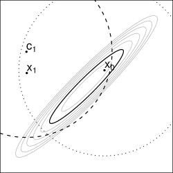
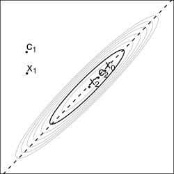
(a)	(b)

Figure 1: (a) The grey lines represent the contours of a two-dimensional distribution; the solid ellipse represents the boundary of the slice. The first crumb, $c_{1}$, is drawn from a spherical Gaussian represented by a dotted circle; a proposal, $x_{1}$, is drawn from a spherical Gaussian centered at $c_{1}$, represented by a dashed circle. $x_{1}$ is rejected because it is outside the solid ellipse. (b) A second crumb, $c_{2}$, is drawn from a reduced-rank subspace, represented by a dashed line. A second proposal, $x_{2}$, is drawn from the same subspace. Since $x_{2}$ is inside the solid ellipse, it is accepted.

Suppose we wish to sample from a target distribution with density function $f(\cdot)$, and the current state is $x_{0}$. In slice sampling, we first draw a slice level, denoted by $y$, uniformly from the interval $[0,f(x_{0})]$. Then, we update $x_{0}$ in a way that leaves the uniform distribution on the slice $\{x|f(x)\geq y\}$ invariant. The resulting stationary distribution of the $(x,y)$ pairs is uniform on the area underneath $f(\cdot)$, and the marginal distribution of the $x$ coordinates has density $f(\cdot)$, as desired.

The crumb framework of slice sampling (Neal,, 2003, §5.2) is a particular way of updating $x_{0}$. First, we draw a crumb from some distribution (to be specified later). Then, we propose a new state from the distribution of states that could have generated that crumb. If the proposal is in the slice, we accept the proposal as the new state. Otherwise, we draw further crumbs and proposals until a proposal is in the slice.

In the shrinking-rank method, the crumbs are Gaussian random variables centered at the current state. To ensure that the uniform distribution on the slice is invariant under state transitions, we will make the probability of starting at $x_{0}$ and accepting a proposal $x_{k}$ the same as the probability of starting at $x_{k}$ and accepting $x_{0}$. This requirement is satisfied if proposal $k$ is drawn from a Gaussian with precision equal to the sum of the precisions of crumbs $1$ to $k$ and mean equal to the precision-weighted mean of crumbs $1$ to $k$.

Further, the precision matrices may depend arbitrarily on the locations and densities of the previous proposals; we take advantage of this by choosing crumb precision matrices that result in state transitions that take large steps along the slice. When the first crumb, $c_{1}$, is drawn, there are no previous proposals providing information to adapt on, so we draw it from a spherical Gaussian distribution with standard deviation $\sigma_{c}$, where $\sigma_{c}$ is a tuning parameter. The distribution for the first proposal, $x_{1}$, is also a spherical Gaussian with standard deviation $\sigma_{c}$, but centered at $c_{1}$ instead of $x_{0}$.

If $x_{1}$ is outside the slice, we can use the gradient of the log density at $x_{1}$ to determine a distribution for $c_{2}$ that leads to a distribution for $x_{2}$ that more closely resembles the shape of the slice itself. In particular, we consider setting the variance of the distribution of $c_{2}$ to be zero in the direction of the gradient, since the gradients are orthogonal to the contours of the log density. If the contour defined by the log density at the proposal and the contour defined by the the slice level are the same shape, this will result in a crumb, and therefore a proposal, being drawn from a distribution oriented along the long directions of the slice. This procedure is illustrated in figure 1.

The nullspace of the subspace the next crumb is to be drawn from is represented by $J$, a matrix with orthogonal, unit-length columns. Let $g^{*}$ be the projection of the gradient of the log density at a rejected proposal into the nullspace of $J$. When $g^{*}$ makes a large angle with the gradient, it does not make sense to adapt based on it, because this subspace is already nearly orthogonal to the gradient. When the angle is small, we extend $J$ by appending $g^{*}/\lVert g^{*}\rVert$ to it as a new column. Here, we define a large angle to be any angle greater than $60^{\circ}\!$, but the exact value is not crucial.

Formally, define $P(J,v)$ to be the projection of vector $v$ into the nullspace of the columns of $J$ (so that it returns vectors in the space that crumbs and proposals are drawn from):

$$P(J,v)=\begin{cases}v-JJ^{T}v&\quad\text{if $J$ has at least one column}\\ v&\quad\text{if $J$ has no columns}\end{cases}$$ (1)

We let $g^{*}$ be the projection of the gradient at the proposal orthogonal to the columns of $J$:

$$g^{*}=P\left(J,\nabla\log f(x_{k})\right)$$

Then we update $J$ if

$$\frac{{g^{*}}^{T}\nabla\log f(x_{k})}{\lVert g^{*}\rVert\,\lVert\nabla\log f(x_{k})\rVert}>\cos 60^{\circ}$$

and the nullspace of $J$ is not one dimensional. This update to $J$ is:

$$J\leftarrow\left[J\quad\frac{g^{*}}{\lVert g^{*}\rVert}\right]$$

To ensure a proposal is accepted in a reasonable number of iterations, if we do not update $J$ for a particular crumb, we scale down $\sigma_{c}$ by a configurable parameter $\theta$ (commonly set to 0.95). Write the standard deviation for the $k$th crumb as $\sigma_{c(k)}$. If we never updated $J$, then $\sigma_{c(k)}$ would equal $\theta^{k-1}\sigma_{c}$. Since we only change one of $J$ or the standard deviation each step, $\sigma_{c(k)}$ does not fall this fast. If the standard deviation were updated every step, it would fall too fast in high-dimensional spaces where many updates to $J$ are required before the proposal distribution is reasonable. As a further refinement, we down-scale $\sigma_{c(k)}$ by an additional factor of $0.1$ when the density at a proposal is zero. Since the usual form of adaptation is not possible in this case, this scaling results in significantly fewer crumbs and proposals on distributions with bounded support.

After drawing the $k$th crumb the mean of the distribution for the next proposal is:

$$x_{0}+P\left(J,\;\frac{\sigma^{-2}_{c(1)}(c_{1}-x_{0})+\cdots+\sigma^{-2}_{c(k)}(c_{k}-x_{0})}{\sigma^{-2}_{c(1)}+\cdots+\sigma^{-2}_{c(k)}}\right)$$

The mean of the proposal distribution is computed as an offset to $x_{0}$, but any point in the nullspace of the columns of $J$ would generate the same result. In that space, the offset of the proposal mean is the mean of the offsets of the crumbs weighted by their precisions. The variance of the proposals in that space is the inverse of the sum of the precisions of the crumbs:

$$\left(\sigma^{-2}_{c(1)}+\cdots+\sigma^{-2}_{c(k)}\right)^{-1}$$

One shrinking rank slice sampler update is shown in figure 2. This will be repeated every iteration of the Markov chain sampler. It could be combined with other updates, but we do not consider this here.

One step in the shrinking-rank method

⬇

$y\leftarrow\operatorname{Uniform}(0,f(x_{0}))$

$k\leftarrow 0$

$\sigma_{c(1)}\leftarrow\sigma_{c}$

$J\leftarrow[\;\;]$

repeat until a proposal is accepted:

$k\leftarrow k+1$

$c_{k}\leftarrow P\bigl{(}J,N(x_{0},\sigma_{c(k)}^{2}I)\bigr{)}$

$\sigma_{x}^{2}\leftarrow\left(\sigma^{-2}_{c(1)}+\cdots+\sigma^{-2}_{c(k)}\right)^{-1}$

$\mu_{x}\leftarrow\sigma_{x}^{2}\left(\sigma^{-2}_{c(1)}(c_{1}-x_{0})+\cdots+\sigma^{-2}_{c(k)}(c_{k}-x_{0})\right)$

$x_{k}\leftarrow x_{0}+P\left(J,N(\mu_{x},\sigma_{x}I)\right)$

if $f(x_{k})\geq y$:

accept proposal $x_{k}$

end (if)

$g^{*}\leftarrow P(J,\nabla\log f(x_{k}))$

if $J$ has fewer than $p-1$ columns and ${g^{*}}^{T}\nabla\log f(x)>\cos(60^{\circ})\cdot\lVert g^{*}\rVert\,\lVert\nabla\log f(x)\rVert$:

$J\leftarrow[\;J\quad g^{*}/\lVert g^{*}\rVert\;]$

$\sigma_{c(k+1)}\leftarrow\sigma_{c(k)}$

else

$\sigma_{c(k+1)}\leftarrow\theta\cdot\sigma_{c(k)}$

end (if)

end (repeat)

Figure 2: This pseudocode represents a single transition in the shrinking rank method with density function $f$, starting from state $x_{0}\in\mathbb{R}^{p}$, and with tuning parameters $\sigma_{c}$ and $\theta$. The mean and variance of the proposals inside the nullspace of $J$ are $\mu_{x}$ and $\sigma_{x}^{2}$. The density of the current slice level is $y$; a real implementation would use the log density. The projection function, $P$, is defined in equation 1. The function $N(\mu,\Sigma)$ generates a multivariate Gaussian with mean $\mu$ and covariance $\Sigma$.

3 Comparison with other methods

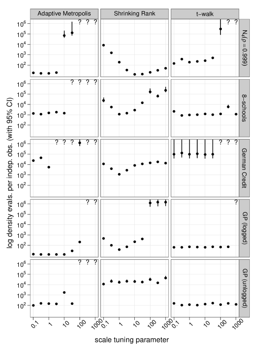
Figure 3: A comparison of three samplers on five distributions using simulations of length 200,000. Log density evaluations per independent observation (lower is better) are plotted against each distribution’s tuning parameter, with asymptotic 95% confidence intervals shown as bars (sometimes too short to be visible). Question marks indicate simulations that had fewer than five distinct observations—too few for the autocorrelation time to be estimated. See section 3 for a description of the distributions and samplers. See Thompson, (2010) for discussion of this type of plot.

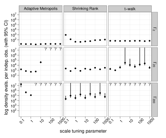
Figure 4: A comparison of three samplers on distributions with uncorrelated Gamma(2,1) marginals. The three distributions have dimensions 2, 20, and 200. Each simulation is of length 60,000.

Figure 3 compares the shrinking-rank method to two other MCMC methods: t-walk and Adaptive Metropolis. The t-walk, described in Christen and Fox, (2010), has a tuning parameter that specifies the separation of the initial coordinate pair. Adaptive Metropolis (Roberts and Rosenthal,, 2009) takes multivariate steps with a proposal covariance matrix chosen based on previous states. Its tuning parameter is the standard deviation of its initial proposal distribution multiplied by the square root of the problem dimension. The shrinking-rank method is described in section 2. The tuning parameter that is varied is $\sigma_{c}$; $\theta$ is fixed at $0.95$.

We compare these methods using five distributions:

• $N_{4}(\rho=0.999)$: a four dimensional Gaussian with highly-correlated parameters; the covariance matrix has condition number 2800.

• Eight Schools (Gelman et al.,, 2004, pp. 138–145): a well-conditioned hierarchical model with ten parameters.

• German Credit (Girolami and Calderhead,, 2011, p. 15): a Bayesian logistic regression with twenty-five parameters. The data matrix is not standardized.

• GP (logged) and GP (unlogged): a Bayesian Gaussian process regression with three parameters: two variance components and a correlation decay rate. Its contours are not axis-aligned. The unlogged variant is right skewed in all parameters; the logged variant, in which all three parameters are log-transformed, is more symmetric.

The shrinking rank method tends to perform well for a wide range of tuning parameters on the first three distributions. Adaptive Metropolis also performs well, as long as the tuning parameter is smaller than the square root of the smallest eigenvalue of the target distribution’s covariance. The recommended value, 0.1, would have worked well for all three distributions. The t-walk works well on the low dimensional distributions, but fails on the higher-dimensional German credit distribution.

The inferior performance of the shrinking rank method on the unlogged Gaussian process regression shows one of its weaknesses: it does not work well on highly skewed distributions because the gradients at rejected proposals often do not point towards the slice. As can be seen by comparing to the logged variation, removing the skewness improves its performance substantially.

Figure 4 shows a set of simulations on distributions of increasing dimension, where each component is independently distributed as Gamma(2,1). For the shrinking rank method and Adaptive Metropolis, multiplying the dimension by ten corresponds roughly to a factor of ten more function evaluations. The t-walk does not scale as well. A similar experiment using standard Gaussians instead of Gamma distributions gives equivalent results.

4 Discussion

The main disadvantage of the shrinking rank method is that it can only be used when the gradient of the log density is available. One advantage is that it is rotation and translation invariant, and nearly scale invariant. It performs comparably to Adaptive Metropolis, but unlike Adaptive Metropolis, adapts to local structure each iteration instead of constructing a single proposal distribution.

An R implementation of the shrinking rank method and the Gaussian process distribution from section 3 can be found at http://www.utstat.toronto.edu/mthompson. A C implementation of the shrinking rank method will be included in the forthcoming SamplerCompare R package. The shrinking rank method and a related method, covariance matching, are also discussed in Thompson and Neal, (2010).

References

- Christen and Fox, (2010) Christen, J. A. and Fox, C. (2010). A general purpose sampling algorithm for continuous distributions (the t-walk). Bayesian Analysis, 5(2):1–20.
- Gelman et al., (2004) Gelman, A., Carlin, J. B., Stern, H. S., and Rubin, D. B. (2004). Bayesian Data Analysis, Second Edition. Chapman and Hall/CRC.
- Girolami and Calderhead, (2011) Girolami, M. and Calderhead, B. (2011). Riemann manifold Langevin and Hamiltonian Monte Carlo. Journal of the Royal Statistical Society B, 73:1–37. arXiv:0907.1100v1 [stat.CO].
- Neal, (2003) Neal, R. M. (2003). Slice sampling. Annals of Statistics, 31:705–767.
- Roberts and Rosenthal, (2009) Roberts, G. O. and Rosenthal, J. S. (2009). Examples of adaptive MCMC. Journal of Computational and Graphical Statistics, 18(2):349–367.
- Thompson, (2010) Thompson, M. B. (2010). Graphical comparison of MCMC performance. Technical Report 1010, Dept. of Statistics, University of Toronto. arXiv:1011.4457v1 [stat.CO].
- Thompson and Neal, (2010) Thompson, M. B. and Neal, R. M. (2010). Covariance-adaptive slice sampling. Technical Report 1002, Dept. of Statistics, University of Toronto. arXiv:1003.3201v1 [stat.CO].