Acceleration of a QM/MM-QMC simulation using GPU

Abstract

We accelerated an ab-initio molecular QMC calculation by using GPGPU. Only the bottle-neck part of the calculation is replaced by CUDA subroutine and performed on GPU. The performance on a (single core CPU + GPU) is compared with that on a (single core CPU with double precision), getting 23.6 (11.0) times faster calculations in single (double) precision treatments on GPU. The energy deviation caused by the single precision treatment was found to be within the accuracy required in the calculation, $\sim 10^{-5}$ hartree. The accelerated computational nodes mounting GPU are combined to form a hybrid MPI cluster on which we confirmed the performance linearly scales to the number of nodes.

I Introduction

GPGPU (General Purpose computing on Graphical Processing Unit) GPU03 ; GPGPU has attracted recent interests in HPC (High Performance Computing) to get accelerations in reasonable prices. Such GPUs with the capability of double precision operations get to be available now. Comfortable environments for developing GPGPU, such as CUDA (Compute Unified Device Architecture)CUDA , also contribute recent intensive trend for applying it to scientific applications with much increased portability. These include computational fluid dynamics, random number generators, financial simulations, astrophysical simulations, signal processings, molecular dynamics, electronic structure calculations, polymer physics etc. Numbers of reports achieving the accerelations by factors of several tens to hundreds are found on the web siteCUDA2 . There has been several attempts using GPGPU applied to ab-initio QMC (Quantum Monte Carlo) electronic structure calculations ONO09 ; ESL09 . These preceding works shows satisfactory efficiencies of acceleration achieved and the possibility of GPGPU challenge in this field. One of the left problem behind would be how to merge the GPGPU with the conventional stream of the development and maintenance of large scale scientific codes in general manner. In pioneering works, GPGPU is sometimes provided in the manner that a typical algorithm is tested in a small scale bench mark code, or some independent ’GPU version’ of the code is developed by re-writting most of the part of the code in CUDA. Our next interest is, however, to apply it to materials simulation programs which are practically used by wider range of users. Such programs has been developed for over tens of years by many contributors working on a lot of branches of functionality of the code. The codes are well designed to be universal to treat wider range of objects from molecules to solids as well as modeled systems such as electron gas. Even for a developer, therefore, it has been not possible to understand the whole part of the code. Developing ’Independent GPU versions’ seems not a practical way to keep harmony with maintenance and version administration of conventional CPU version of the codes. In this paper we identified the bottle neck of original CPU version firstly and then developed CUDA version only on the corresponding subroutine being tiny part of the whole code. The main body of the code is written in Fortran90 (F90) and we combined the CUDA subroutine at object code level. Users can switch back to the original CPU version of the subroutine if GPU is not available.

Another different point from preceding studies are that GPGPU here is devoted to accelerate single core performance, being possible to coexist with current MPI (Message Passing Interface) implementation. In many QMC codes NEE10 ; QMCPACK , MPI parallelization is used to divide up whole sampling tasks into processor cores. In preceding works GPU is used so that the parallelized tasks are distributed into GPU cores instead of CPU cores. Improved performance was obtained because the number of cores in GPU exceeds that in CPU. We didn’t take this way because of the following reasons: Firstly, in practical codes, the parallelized task contains much larger processes requiring larger memory capacities than in limited-purposed benchmark codes. We don’t expect the task is possible to be put in threads running on GPU. As another reason we point out the fact that the current CPU-MPI implementation is inherently successful for QMC because of less frequent communications between processor nodes. When the number of cores gets massive it is, nevertheless, pointed out the problems such as the load balancing or other bottle neck arising etc. These problems would similarly occur even when the parallel cores are replaced by GPU. Larger number of dense coupled processor cores in GPU compared with CPU does not so much matter in our QMC case because inter-core communication is not the bottle neck. In this work we kept conventional MPI parallelization over CPU cores. GPU many-core feature is exploited to speed up each sampling task which is distributed on each CPU core by MPI, being similar to the idea of hybrid parallelization such as Open-MP combined with MPI.

As a proper example we applied GPGPU to a QM/MM (Quantum Mechanics / Molecular Mechanics) calculation called as ’FMO-QMC’ calculationMAE07 . In this case the bottle neck of single core performance is identified to the part evaluating electrostatic fields due to given charge densities. The field is constructed by large amount of summations in a loop being fit to GPU acceleration by its many-core feature, finally getting 23.6 times faster performance when we compare the performance on a (single core CPU double precision + GPU with single precision) with that on a (single core CPU with double precision). We also confirmed the acceleration can be in harmonic with that by conventional CPU-MPI parallelization. As is given in the discussion section later, there would still be more space to improve the acceleration by combining OpenMP with the present work, or by using a scheme where the GPU is shared by the MPI processes running on the same node. Here we report a work as a first step towards an efficient acceleration of the code by replacing only the ’hotspot’ with CUDA-GPU.

The paper is organized as follows. In §II we briefly summarize the subjects required here, such as VMC (Variational Monte Carlo method), FMO (Fragment molecular method), and GPGPU. In §III we describe details how to measure the performance, namely the system to be evaluated and the coding structures. Results are shown in §IV and discussions are given in §V.

II Methodologies

II.1 VMC

In ab-initio calculations the system to be considered is specified by a given hermitian operator $\hat{H}$ called as HamiltonianPAR94 . The operator includes information about positions and valence charge of ions, the number of electrons, and the form of the potential functions in the system. The fundamental equation at electronic level, called as many-body Schrödinger equation, takes the form of a partial differential equation with the operator $\hat{H}$ acting on a multivariate function $\Psi\left(\vec{r}_{1},\cdots,\vec{r}_{N}\right)$, called as many-body wave function, where $N$ denotes the number of electrons in the system. The energy of the system, $E$, is obtained as the eigenvalue of the partial differential equation. The equation has the variational functional HAM94 ,

$$E = \frac{\int\Psi^{*}\hat{H}\Psi\,d{\vec{r}_{1}}\cdots d{\vec{r}_{N}}}{\int\Psi^{*}\Psi\,d{\vec{r}_{1}}\cdots d{\vec{r}_{N}}}$$ (1)

$$= \frac{\int|\Psi|^{2}\cdot\Psi^{-1}\hat{H}\Psi\,d{\vec{r}_{1}}\cdots d{\vec{r}_{N}}}{\int|\Psi|^{2}\,d{\vec{r}_{1}}\cdots d{\vec{r}_{N}}},$$

which is minimized when the above integral is evaluated with $\Psi$ being an exact solution of the eigen equation. For a trial $\Psi$ the functional can be evaluated as an average of the local energy, $E_{L}\left(\vec{r}_{1},\cdots,\vec{r}_{N}\right)=\Psi^{-1}\hat{H}\Psi$ over the probability density distribution $p(\vec{r}_{1},\cdots,\vec{r}_{N})=|\Psi|^{2}/\int|\Psi|^{2}\,d{\vec{r}_{1}}\cdots d{\vec{r}_{N}}$. In VMC the average is evaluated by Monte Carlo integration technique using the Metropolis algorithm to generate sample configurations $\left\{\vec{R}_{j}\right\}_{j=1}^{r}$ distributed by $p(\vec{r}_{1},\cdots,\vec{r}_{N})=p(\vec{R})$, where $\vec{R}$ denotes a configuration $(\vec{r}_{1},\cdots,\vec{r}_{N})$ as

$$E=\sum_{j=1}^{r}{E_{L}\left(\vec{R}_{j}\right)}\ ,$$ (2)

with $r$ being the order of millions typically. Trial function $\Psi$ is improved so that the integral is numerically minimized. Several functional forms for $\Psi$ are possible, amongst which we took commonly used Slater-Jastrow type wave function FOU01 . Since each $E_{L}\left(\vec{R}_{j}\right)$ can be evaluated independently the summation over $j$ can be distributed over processors by MPI with enough high efficiencyFOU01 . In this work GPGPU is used to accelerate each $E_{L}\left(\vec{R}_{j}\right)$ evaluation, not applied to this parallelization. For VMC we used ’CASINO’ program packageNEE10 with the extended functionality for FMO-QMCMAE07 as described in the next section.

II.2 FMO method

FMO (Fragment Molecular Orbital) method, KIT991 ; KIT992 as a sort of QM/MM method, is devised to treat larger biomolecules in ab-initio electronic structure calculations. To accommodate in available memory capacities with affordable computational cost, the whole system is divided into several sub-systems called as fragments. Only within the fragments the electrons are treated fully by quantum mechanics while the contributions from other fragments are replaced into classical electrostatic fields formed by charge densities of electrons and ions. While molecular orbital methods (MO) or Density Functional Theory (DFT) calculations are commonly used to evaluate sub-systems, QMC, instead, is expected to be powerful to get more reliable estimation of electronic correlations which is believed to play important roles in biomolecules. In the framework, FMO-QMCMAE07 , the additional task to evaluate electrostatic fields at each Monte Carlo step causes considerable speed-down by around 50 times longer CPU time than that of normal QMC with the same system size.

When we divide the system into $L$ sub-systems, the energy of the whole system, $E_{\rm All}$, is approximately evaluated as,

$$E_{\rm All} \approx \sum_{i=1}^{L-1}\sum_{j=i+1}^{L}E_{ij}+(L-2)\sum_{i=1}^{L}E_{i}\ ,$$ (3)

from the energies calculated for each sub-system $E_{i}$, and those for pairs of sub-systems $E_{ij}$. These ’fragment energies’ are evaluated under the electrostatic fields, $U_{\rm ES}\left({\vec{r}}\right)$, due to other fragments. In FMO-QMC, $U_{\rm ES}\left({\vec{r}}\right)$ should be constructed at every Monte Carlo step with updated electronic positions, $\vec{r}=\vec{r}_{\rm new}$. Charge densities to form the field are given as input files as $\left\{Z_{\beta}\right\}$ being valence of nuclei and $\left\{\rho\left(\vec{r}_{m}\right)\right\}$ being charge intensities of each spatially discretized cell on the fragment (index $\beta$ runs over $K$ nuclei at $\vec{R}_{\beta}$, and $m$ over $M$ cells centered at $\vec{r}_{m}$ in the fragment). The field is hence given as

$$U_{\rm ES}\left({\vec{r}_{\rm new}}\right) = \sum_{m=1}^{M}\frac{\rho\left({\vec{r}_{m}}\right)}{\left|{\vec{r}_{\rm new}}-{\vec{r}_{m}}\right|}-\sum_{\beta=1}^{K}\frac{Z_{\beta}}{\left|{\vec{r}_{\rm new}}-{\vec{R}_{\beta}}\right|}$$ (4)

$$= U_{\rm ES}^{\rm ele.}\left({\vec{r}_{\rm new}}\right)-U_{\rm ES}^{\rm nuc.}\left({\vec{r}_{\rm new}}\right)\ .$$

While $K$ amounts to dozens, $M$ gets to around hundreds thousand, resulting the evaluation of $U_{\rm ES}^{\rm ele.}$ being quite heavy. Figure 1 visualizes an image of the evaluation.

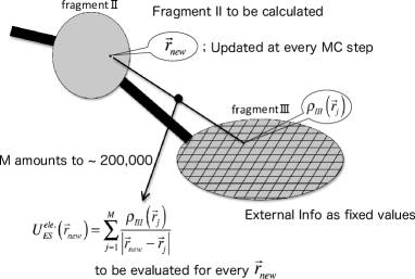
Figure 1: Evaluation of electrostatic fields in FMO-QMC calculation.

The evaluation is the most time consuming part of FMO-QMC, for which we applied GPGPU acceleration.

II.3 GPGPU

GPGPU exploits hundreds of processing cores in GPU which are originally designed for graphical data processing. Its performance on single precision operations gets to tens times faster than that of commonly used CPU. Comfortable code-developing environments are available recently, such as CUDA, by which we can develop GPU codes in more universal manner written in language being similar to C language with some extended definitions of variables and functions for GPU. In GPGPU a program consists of host codes and the kernel codes, former of which run on CPU while the latter on GPU getting data sent by the host code from CPU. Frequent data transfer between the host and the kernel should be avoided because the transfer is made via bus with relatively low speed. Less transfers to and more operations on GPU are preferable for getting better performance.

In GTX275GTX275 , a GPU we used here, there are 30 Streaming Multiprocessors (SM). Each SM includes eight Streaming Processors (SP) which are used as a smallest processor unit in GPGPU, as shown in Fig. 2. Single precision operations can be handled independently on each SP while double precision requires to be processed on a DPU (Double Precision Unit) located on each SM. This makes double precision operations slower by around a factor of eight. Instructions are interpreted on a SM at every four clock cycles and then executed on eight SPs within the SM. 32 threads (4 cycles $\times$ 8 SP), therefore, forms a unit of SIMD (Single Instruction Multiple Data) operation, called as a warp.

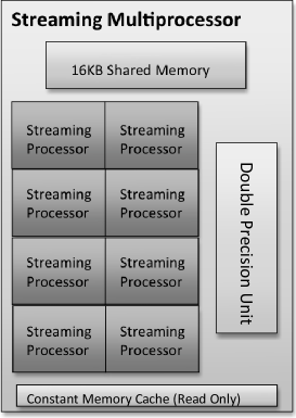
Figure 2: Schematic picture of a Streaming Multiprocessor (SM).

In GPU, threads are administrated in a layered structure. Threads are labeled by three dimensional indices within a block. Similarly, blocks are labeled by two dimensional indices within a grid, though the grid is not used in the present study. Each block is processed by a SM, not by several. If the number of blocks exceeds that of SM, the blocks are processed by the SM in due order. It is therefore usual manner to select the total number of blocks to be a multiple of the number of SM. Since a warp is formed by 32 threads, the total number of threads would be chosen as a multiple of 32. From the view point of memory latency it is said a multiple of 64 is preferred. Practically the total number of threads is chosen so that the memory capacity required for each thread can be affordable within a SM, otherwise the performance gets considerably worse.

Table 1 shows various kinds of memories available in GPU. The list contains only those relevant to this study, excluding texture memory. Off-chip memories are located within GPU board but not on the device chip. They have larger capacities and are accessible from hosts but lower speed in general. On-chip memories are complementary, namely with higher speed and lower capacity.

	Location	Cache	R/W	Availability	Data maintained
Register	On-chip	-	R/W	within a thread	during a thread
Local memory	Off-chip	No	R/W	within a thread	during a thread
Shared memory	On-chip	-	R/W	from all threads	during a block
				within a block
Global memory	Off-chip	No	R/W	from all hosts	during host code
				and threads	maintains
Constant memory	Off-chip	Yes	R	from all hosts	during host code
				and threads	maintains

Table 1: Various kinds of memory in GPU relevant to this study. R and W stand for readable and writable, respectively.

In GTX275 there are 16,384 registers available for each SM, and variables defined within kernel codes can be stored there. When registers are run out, data are evacuated to off-chip local memories and newer data are stored into register. The local memory is about 100 times slower than register and so it is important to save register for better performance. Data to be sent to GPU is firstly stored on a off-chip global memory by a host code and then loaded by a on-chip shared memory in usual manner. Larger capacity is available in global memories ranging from 512MB to 1GB depending on the products. Again the off-chip global memory is about 100 times slower. Though they are similarly depicted in Fig. 2, the shared memory is on-chip while the constant memory is off-chip. Each SM has a 16KB shard memory which is accessible from all threads within a block. Though 64KB constant memory is off-chip, it can be accessed with higher speed from all threads using cache on each SM (constant cache). This is read only so convenient to store constants defined in kernel codes. A data load from global memories is executed in parallel manner by 16 threads simultaneously in GTX275, corresponding to a half of a warp. When the addresses accessed by parallel threads are sequential, the access speed is accelerated by the order of the number of threads. This is called as ’coalescing’ and very important in the performance achieved by the present study.

III Experimental setup

As a benchmark system for FMO-QMC, we took a glycine trimer to measure the performance of GPGPU. The system is divided into three fragments in this caseMAE07 . The computational time required to evaluate the energy of the smallest fragment (’fr1’ in ref MAE07 ), corresponding to the term $E_{1}$ included in the second summation in Eq.(3), is measured and compared by CPU and GPU. Detailed setup of the trial wave function such as basis sets, Jastrow functions, and variational optimizations etc. are the same as given in the ref.MAE07 . Computational cost for this fragment to achieve the statistical error required for meaningful arguments in the context of quantum chemistry, as published in reference MAE07 , is estimated around 50 days with single core, 13,000 times more Monte Carlo steps than the present case. In this work we took shorten run for benchmark, making it be finished within around 300 sec. by single core. Note that the ’accuracy’ argued in the present study is different from the statistical error because we fixed the seed for the random number generator, namely we took a deterministic system to be compared with each other in this work.

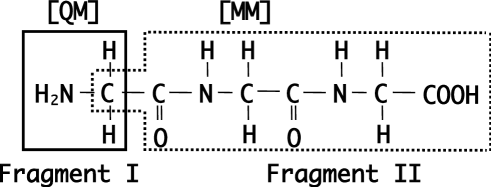
Figure 3: Fragmentation of glycine trimer used hereMAE07 . QM means the fragment treated by quantum mechanical dynamics while MM the part handled as an environment for QM giving classical electrostatic field.

The FMO-QMC code is an extension of ’CASINO’ QMC code NEE10 written in F90, while CUDA itself provides only the C-language compiler. Though there appears commercial fortran compilers for GPU such as PGI Accelerator CompilersPGI09 recently, we didn’t take them. Instead we combined the F90 part and CUDA part at the object file level. The structure of the codes we developed is shown in Fig. 4.

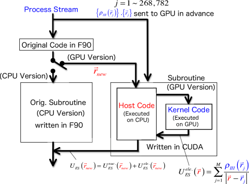
Figure 4: Structure of the code.

We applied GPGPU only to the most time consuming subroutine, namely that evaluating $U_{\rm ES}\left(\vec{r}\right)$. As shown in Fig. 4 we developed a detour leading to GPU version of the subroutine written in CUDA, consisting of the host and the kernel code. The host code is called from the main body written in F90, getting the updated particle position, $r_{\rm new}$, at each MC step. The host code then calls the kernel code on which the electrostatic field, $U_{\rm ES}^{\rm ele.}\left(\vec{r}_{\rm new}\right)$, is calculated to be sent back to the host code. For more efficiency, the host code calculates $U_{\rm ES}^{\rm nuc.}$ independently on CPU, which can be finished until it gets $U_{\rm ES}^{\rm ele.}$ from GPU. These are summed to form $U_{\rm ES}$, which is then sent back to the main body in F90. For evaluating $U_{\rm ES}^{\rm ele.}$ on GPU, cell positions and charge densities, $\left\{\rho\left(\vec{r}_{j}\right)\right\}$, should be stored on memories in GPU. The data is large but read-only, so the data transfer to GPU is required only once at the beginning of a run, not consuming computational cost relative to the whole CPU time. The data communication with GPU at each MC step therefore deals only with $\vec{r}_{\rm new}$ (input) and $U_{\rm ES}^{\rm ele.}$ (output), getting cheaper data-transfer cost.

The summation to form $U_{\rm ES}^{\rm ele.}$ in Eq. (4) is divided into sub-summations as

$$U_{\rm ES}^{\rm ele.}=\sum\limits_{j=1}^{M}{u_{j}}=B\left[1\right]+B\left[2\right]+\cdots+B\left[{N_{B}}\right]\ ,$$ (5)

and distributed to each block (total $N_{B}$ blocks) on GPU for acceleration. Denoting $N_{\rm th}$ being the number of threads within a block, and $N_{\rm loop}$ being the number of loops per thread,

$$B\left[m\right]=\sum\limits_{j=1}^{N_{\rm th}\times N_{\rm loop}}{b_{j}^{\left(m\right)}}\ ,$$ (6)

where $\left\{{b_{j}^{\left(m\right)}}\right\}\in\left\{{u_{j}}\right\}$ are the elements of summation treated by the block $m$. Total number of terms, $M$ = 268,782, is then distributed to $\left(N_{B}\times N_{\rm th}\right)$ threads, within which $N_{\rm loop}$ loops are performed so that $M\leq\left(N_{B}\times N_{\rm th}\times N_{\rm loop}\right)$. In this work we choose $N_{B}$=120 as a multiple of the number of SM (= 30 for GTX275), $N_{\rm th}$ = 256 as a multiple of warp size, 32, resulting in $N_{\rm loop}$=9.

$\left\{\rho\left(\vec{r}_{j}\right)\right\}$ is initially stored in the global memory. Getting $\vec{r}_{\rm new}$ from CPU, it is put in the constant memory, and then evaluated to form $\left|\vec{r}_{\rm new}-\vec{r}_{j}\right|$, stored on the register. Each sub-summation $B\left[m\right]$ is stored in the shared memories to contribute to the total summation by reduction operation. Using the read-only constant memory with higher latency for $\vec{r}_{\rm new}$ is found to be essential tip for the present achievement, because $\vec{r}_{\rm new}$ is the fixed quantity during the construction of $U_{\rm ES}$.

Table 2 summarizes the specification of a computational node we used for the experiments. To measure parallel performance of GPU we used a cluster consisting of four nodes connected by a 100 Mbps switching hub. On each node an Intel Core i7 920 processorINT09 and a GPU is mounted on a mother board. Hyper-Threading HTT in Core i7 processor is turned off, using it as a four-core CPU. Specs of GeForce GTX 275GTX275 is summarized in Table 3. Compute Capability specifies the version of hardware level controlled by CUDA, above ver.1.3 of which supports double precision operations. For Fortran/C codes we used Intel compiler version 10.1.018 for both using options, ’-O3’ (optimizations including those for loop structures and memory accesses), ’-no-prec-div’ and ’-no-prec-sqrt’ (acceleration of division and square root operations with slightly less precision), ’-funroll-loops’ (unrolling of loops), ’-no-fp-port’ (no rounding for float operations), ’-ip’ (interprocedural optimizations across files), and ’-complex-limited-range’ (accerelation for complex variables). For CUDA we used nvcc compiler with options ’-O3’ and ’-arch=sm_13’ (enabling double precision operations).

CPU	Intel Core i7 920 2.66 GHz (Max 2.80 GHz)
GPU	GeForce GTX 275 $\times$ 1
Motherboard	ASUS RAMPAGE II GENE (Intel X58 chipset)
Memory	DDR3-10600 2GB $\times$ 6
OS	Linux Fedora 10
CUDA	CUDA version 2.3
Fortran/C Compiler	Intel Fortran/C Compiler 10.1.018
MPI	mpich2-1.2.1
CUDA Compiler	NVIDIA CUDA Compiler (nvcc)

Table 2: Setup of a computational node.

Compute Capability	1.3
Global memory	895 MB
Number of SM	30
Number of SP	240
Clock of SP	1.404 GHz
Constant memory	64 KB
Shared memory	16 KB per block
Warp size	32
Max number of threads	512 per block
Memory band width	127 GB per sec.

Table 3: Specs of GPU.

IV Results

Single core performances we measured are tabulated in Table 4. The values shown are the CPU time for whole calculation including initial data loads onto GPU, evaluated by averaging over 100 individual runs. Compared with the normal CPU calculation with double precision (341.14 sec.), we finally achieved 23.6 (11.0) times faster calculations with single (double) precision by GPU with coalescing. For more acceleration of the double precision calculation we also tried replacing our division operation into that provided as a CUDA function (SFU : Super Function Unit) but no remarkable speed up observed. In single (double) precision results the observed deviation in the final ground state energy from that by the original CPU/double precision calculation was within $10^{-5}$ ($10^{-12}$) a.u. This assures the capability of single precision calculations by GPGPU to provide the results within the chemical accuracy $\Delta E\sim 10^{-3}$ a.u. with substantially speeding up, as a particular interest.

Table 4: Comparison of CPU time between single core CPU and GPU. All values are given in sec.

	Single Precision	Double Precision
CPU(single core)	-	341.14
GPU/Coalescing	14.44	30.89
GPU/Incoalescing	44.37	48.75

As shown in Table 4, the best performance is achieved by the code properly written to get coalescing. The results shown in the row of ’Incoalesing’ are obtained by a naive construction of the summation in Eq. (6),

$$B\left[m\right]=\left[{b_{1}^{\left(m\right)}+b_{2}^{\left(m\right)}+\cdots+b_{N_{\rm loop}}^{\left(m\right)}}\right]+\left[{b_{N_{\rm loop}+1}^{\left(m\right)}+\cdots+b_{2N_{\rm loop}}^{\left(m\right)}}\right]+\cdots\\ \ ,$$ (7)

where $\left[\cdots\right]$ corresponds to each sub-summation evaluated within each thread. In this construction the threads access to a global memory to retrieve $\left({b_{1}^{\left(m\right)},b_{N_{\rm loop}+1}^{\left(m\right)},b_{2N_{\rm loop}+1}^{\left(m\right)},\cdots}\right)$, for example at the first step of the loop, lacking the sequence in addresses to be referred. By improving the construction as,

$$B\left[m\right] = \left[{b_{1}^{\left(m\right)}+b_{1+N_{\rm th}}^{\left(m\right)}+\cdots+b_{1+\left({N_{\rm loop}-1}\right)N_{\rm th}}^{\left(m\right)}}\right]+\left[{b_{2}^{\left(m\right)}+b_{2+N_{\rm th}}^{\left(m\right)}+\cdots+b_{2+\left({N_{\rm loop}-1}\right)N_{\rm th}}^{\left(m\right)}}\right]+\cdots$$ (8)

$$+\left[{b_{N_{\rm th}}^{\left(m\right)}+\cdots+b_{N_{\rm th}+\left({N_{\rm loop}-1}\right)N_{\rm th}}^{\left(m\right)}}\right]\ ,$$

we can make it to be sequential memory access, getting coalescing efficiency. This brought about three times faster evaluation in single precision calculation. Without coalescing we could get little acceleration (less than 10$\%$) in single precision calculation compared with double precision, as seen in Table 4.

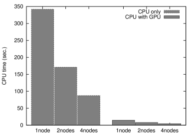
Figure 5: Comparison of CPU time between multi-core CPU and single precision MPI-GPU.

Table 5: MPI performances with Double precision. All values are given in sec.

	CPU only	CPU with GPU
		Double prec(Coalesing).	Single prec.
1 MPI process	341.14 (1CPU/1core)	30.89	14.44 (1CPU & 1GPU, 1core/CPU)
2 MPI processes	171.28 (1CPU/2cores)	15.70	7.68 (2CPU & 2GPU, 1core/CPU)
4 MPI processes	87.01 (1CPU/4cores)	8.20	4.26 (4CPU & 4GPU, 1core/CPU)

Parallel performances are evaluated and compared with multi-core CPU, as summarized in Table 5 and Fig. 5. Even the worst case of GPU (double precision/single core/incoalesing) (48.75 sec.) is still faster than four-core CPU calculation (87.01 sec.). For ’CPU only’ calculations we measured the performance within a node (and hence the MPI runs within a CPU), while for GPU parallel (’CPU with GPU’), $N$-MPI runs on $N$ nodes and then only a processor core is used in a CPU on a node. Both in ’CPU only’ and ’CPU with GPU’, measured performances roughly scale to the number of processor cores, showing high parallel efficiency of the Monte Carlo simulation even with cheaper 100 Mbps switching hub. The results support that the acceleration of single core performance by GPU can be in harmony with the MPI parallel acceleration.

V Discussions

Table 6 shows a rough estimation of performances expected in devices used here, just by their numbers of cores and clock frequencies.

Table 6: Estimation of Performances of devises used here.

	Clock Freq.	# of Cores	Performance
CPU	2.66 GHz	4 cores	42.56 GFLOPS
GPU (Double Prec.)	1.404 GHz	30 cores	84.24 GFLOPS
GPU (Single Prec.)	1.404 GHz	240 cores	1010.88 GFLOPS

Values to be compared with our achieved factor 23.6 (11.0) for single (double) precision would be evaluated as follows: Since we got the factors based on CPU single core performance, 42.56/4=10.64 GFLOPS, we hence expect the upper limit of the acceleration factor being around 94.9 ( = 1010.88/10.64) [7.9 ( = 84.24/10.64)] for single [double] precision operation.

The peak GPU performance for single precision, 1010.88 GFLOPS, is simply estimated as 1.404 GHz $\times$ 240 cores$\times$ 3, where the last factor, three, is the maximum possible number of operations at one clock cycle. Such a peak case occurs only when all the operations consist of fused multiply-add and a multiply operation, which fit to the execution by SFU pipeline. One cannot expect such an extreme case generally and then it is more likely being around 337 GFLOPS in practical cases by dropping the last factor, three. Correspondingly the ideal limit of acceleration factor in the practical situation for single precision would be evaluated as 31.7 to be compared with our 23.6. The ideal limits would be achieved when a code all consists of operations. Memory accesses contained frequently in the actual codes would lower the performance, accounting for the discrepancy. This would also be supported by the fact that the single precision performance strongly depends on the coalescing.

The reduced performance in the double precision compared with the single precision mainly comes from the fact that a DPU is available only on each SM, not on SP. Again, only if the code all consists of double precision operations, the reduction would occur but in the actual code it wouldn’t, giving the possibility for acceleration factor being beyond 7.9. This would account for our achievement with coalescing being the factor of 11.0. The excess factor $7.9/11.0=0.72$ might be attributed to insufficient tuning on the original CPU code. If so our achievement in single precision calculation would be reduced as $23.6\times 0.72=17.0$, being still a satisfactory efficiency. For more reliable/fair estimation of the acceleration factor, the original CPU version should be optimized enough, though it is generally difficult to say how much one’s code is optimized. For reference we took a profiling of the code using ’OProfile’ profiler oprofile . Measured on Intel Core2Quad/9550, the bottle-neck subroutine of CPU version (that shown in Fig. 4) achieved 0.77 GFlops with 97.35% of the whole CPU time. The value is obtained from the count of operations divided by the execution time consumed by the subroutine, corresponding only to less than 2% of the peak performance of the processor, 45.28 GFlopscore2 . It is, however, known that OProfile tends to underestimate the performance because it cannot correctly take into account SSE. For calibration we measure the performance of LINPACK in the same way, giving 9.4 GFlops by OProfile, while LINPACK itself reports 21.41 GFlops in its output, supporting our ’less than 2%’ might be underestimated. Another possible reason for such low performance would be because of the dividing operation to get $1/r$ potential. The peak performance based on multiple/add operation would be reduced for the dividing operation, and hence corrects the measured performance upward.

For more information about how much the original CPU code optimized, we examined the dependence on compilers. Using PGI fortran compiler (ver. 11.1), our best performance is obtained with options, ’-03’, ’-fastsse’ (optimization for SSE/SSE2), ’-tp nehalem-64’ (for Intel Core i7(nehalem)), and ’-Mfprelaxed’ (accelerating of dividing and squared root operations with reduced accuracies), getting 343.51 sec. for 1CPU/1core compared with 341.14 sec. by Intel compiler. This insensitive result is in contrast to the case when we compared them for a typical example run of CASINO without FMO, namely without running through the bottle-neck subroutine considered here, showing 1.62 times faster optimization by intel than that by PGI. This would also imply that the bottle-neck has enough simple structure with little possibility to be optimized further at compiler level.

The acceleration factor by the coalescing is said to be around 10.0 at most. Though our achievement in total CPU time was only 3.07 as shown in Table 4, our profiler analysis indicates that the execution time consumed only by the kernel code is accelerated around the factor of 6.0 by the coalescing with glb_64b and glb_128b being increased from zero, being a satisfactory efficiency.

Reduced/limited performance in double precision calculations is expected to be improved in next generation GPUsFermi09 .

Table 7: Comparison of performances by GTX480 and GTX275

	GTX480		GTX275
	Double prec.	Single prec.	Double prec.	Single prec.
1 MPI process	18.28	12.58	30.89	14.44

We did a brief check on the dependence of performance on the generation of architecture using GeForce GTX480 as shown in Table 7. GTX480 is a product employing the latest Fermi architectureFermi09 on which the double precision performance is much improved. In this quick check we used the same kernel code, not optimized specific for GTX480. Because of the available matching to drivers and OS, the test condition is not the same, using CUDA version 3.1 and Linux Fedora 12. Even without further tuning for GTX480 the performance is considerably improved, especially for double precision being 1.69 times faster. This comes from the increased number of double precision operation unit in Fermi. The number is 16 per SM in GTX480 while one for GTX275. Having 15 SMs in total, the new architecture has 240 double precision operation units, compared to 30 for GTX275. It is then expected eight times faster performance though, NVIDIA limits it to be 1/4 of that for this product. It leads to twice faster performance as expected, well compared to our achievement, 1.69. The limitation is removed only for the product line, Tesla C2000 series, on which more performance is expected. Another possibility for further improvement would be to use hybrid parallelization. During the CPU-GPU operation in the present implementation only a processor core in CPU is used leaving other three cores unused. There are still more spaces to increase our efficiency by applying OpenMP, for example, to the host code shown in Fig. 4 to be exploited unused cores.

Though for practical usage of the application the code is indeed accelerated by the factor of 23.6, we point out the statement ’how much the GPU accelerates the calculation’ includes the ambiguity which easily leads to misunderstandings especially when it is argued in the context of architecture performance. Our achieved factor, 23.6, would be reduced to be around 2.0 depending on the context, as tabulated in Table 8: We first note that our measurement for single precision is not a ’clearcut’ comparison because we compared [CPU main body (double prec.) + GPU subroutine (single prec.)] to [CPU main body (double prec.) + CPU subroutine (double prec.)]. More ’natural’ choice for the comparison would be to use original CPU version with single precision. As excused in §I, however, it is practically impossible to get such a whole single precision version of the original code which is widely used and developed/maintained in double precision, being the reason why we took such a setting for the comparison. Nevertheless, it is worth pointing out that the single precision performance of original CPU code, if it were available, would give more information about how much the original code is optimized as the following reason: If the original code is well optimized to fit to SIMD enough, the single precision version can give twice faster CPU time at most because SIMD can accommodate twice operations for single precision than for double precision. In such ideal limit we could measure how much the original code has been optimized by observing how close the CPU time to the halved value of that by double precision. If it is not closer it would imply that not all the operations are fit to SIMD and hence the original would have more spaces to be optimized. If the code is well optimized it might be possible to get less than the halved because for single precision the cache is more effectively working with less cache miss. That for CPU+GPU version would also be reduced a bit by replacing the CPU part by single prec. version, but from the fact that the bottle neck is the GPU part, we expect its CPU time is not so changed. Then we estimate a halved value of 23.6, 11.8 as such an extreme limit estimation of the acceleration factor on the ’natural’ definition, as shown in the third raw of Table 8 as the lowest estimate. However, based on practical experiences, it is quite unlikely to get such an ideal situation having halved CPU time of double precision by replacing it to singleTOM10 . For reference, LINPACK performance measured on Core i7-860 with Intel C Compiler 11.073 showed only 3-4% increase in FLOPSTOM10 by replacing double precision to single. Taking 4% as an estimate we also put 22.70 in the third raw of Table 8 as the highest estimate.

If we further includes the possibility of CPU to be accelerated by its multicore into the definition of ’the comparison between a GPU and a CPU’, the factor should be divided by four, the number of cores in our case, getting 11.8/4 = 2.95 for single precision and 11.0/4 = 2.75 for double precision. If we argue the ’merit factor’, namely how much the acceleration obtained by adding a GPU on a motherboard instead of an extra CPU (dual CPU setup), the factor is further divided by two. In this measure we get 1.38 for double prec. and 1.48 for single prec. This merit factor would be accompanied by the further note that adding an extra CPU can achieve the acceleration without the human effort of writing the ’Nvidia-specific’ version of the subroutine. In the above context, the ideal limit (1010.88 GFLOPS) and practical limit (337 GFLOPS) of the GPU performance are translated into the merit factors of 5.93 - 11.4 and 1.98 - 3.81, respectively.

Table 8: Several possible ways to represent acceleration factor. SP (DP) stands for single (double) precision, respectively.

Reference to estimate	SP on GPU	DP on GPU	Remarks
accerelation factor
CPU/SingleCore/DP	23.6	11.0	Practically observed here
CPU/SingleCore/SP	11.8 - 22.70	N/A	True comparison for SP
			(ideally estimated)
CPU/MultiCore/SP	2.95 - 5.68	2.75	Comparison between
			multicore CPU and GPU
CPU plus added	1.48 - 2.34	1.38	”Merit factor”
CPU/MultiCore/SP			5.93 - 11.4 (ideal limit)
instead of GPU			1.98 - 3.81 (practical limit)

System size dependence of the present acceleration should be mentioned. For the present QM/MM methods (FMO-QMCMAE07 ), the size of MM part matters for the total CPU cost via the construction of $U_{\rm ES}$. This is in contrast to SCF (self-consistent fieldSZA89 ) based methods such as FMO-SCFMAE07 , for which QM size usually matters. The present system shown in Fig. 3 provides the largest MM size among the fragmentations of the system, and hence the most expensive CPU time. The CPU cost scales to the total loop size $M$ which is roughly proportional to the cube of the MM system size. QMC calculation itself is known to have such scaling that the CPU time proportional to $N_{\rm QM}^{2}$ - $N_{\rm QM}^{3}$, where $N_{\rm QM}$ stands for QM system size NEE10 . In FMO-QMC more than 90% of the CPU time is spent for the evaluation of MM part, namely the construction of $U_{\rm ES}$. Then we expect the total CPU time is almost dominated by MM size. The present MM size, 19 atoms with 84 electrons, is within the range of usual choice commonly used for FMO applied to amino acids, so the results estimated here give universal trend for other FMO-QMC systems to some extent. The factor of the acceleration is expected to be unchanged or a bit improved when the MM size gets larger for the following reasons: The acceleration is achieved by dividing the total loop size into smaller ones each of which processed on parallel threads on GPU. Such ’barrel processing’ gets more advantage as the number of threads increased with more efficiency to hide the latency. The number of variables transferred between CPU and GPU during main calculation, $\vec{r}_{\rm new}$ and $U_{\rm ES}$, does not depend on the MM size, and hence no increase in communication cost. The capacity to accomodate $\left\{\rho\left(\vec{r}_{j}\right)\right\}$ increases but is kept within the range of the global memory which has enough space. Registers and shared memories are used to accommodate each sub-summation, so their capacity limitation does not matter for the choice of MM size.

VI Concluding Remarks

We applied GPGPU to accelerate the single core performance on a QMC code combined with a QM/MM treatment in FMO method. Only the bottle-neck subroutine of the code is translated to be written in CUDA and performed on GPU. A large scale summation in the part is divided into sub summations distributed to threads running on many cores in GPU, getting 23.6 (11.0) times faster performance in single (double) precision when we compare the performance on a (single core CPU double precision + GPU with single precision) with that on a (single core CPU with double precision). The accuracy in single precision calculation was confirmed to be kept within the required extent (chemical accuracy, $\sim$0.001 hartree in energy). Such accelerated nodes are combined to build a MPI cluster, on which we confirmed the MPI performance scaling linearly with the number of nodes upto four. Achieve factors of the acceleration are compared with ideal limits, and possible accounts for the discrepancy are investigated, putting the present work as a first step towards further efficient acceleration of such strategy replacing only the most time consuming subroutine with CUDA-GPU one.

VII Acknowledgments

Authors would like to thank Hisanobu Tomari and Daisuke Takahashi for their valuable comments on CPU single precision performance. The computation in this work has been partially performed using the facilities of the Center for Information Science in JAIST. Financial support was provided by Precursory Research for Embryonic Science and Technology, Japan Science and Technology Agency (PRESTO-JST), and by a Grant in Aid for Scientific Research on Innovative Areas ”Materials Design through Computics: Complex Correlation and Non-Equilibrium Dynamics (No. 22104011)” (Japanese Ministry of Education,Culture, Sports, Science, and Technology ; KAKENHI-MEXT) for R.M.

References

-
(1)
gACM Workshop on General Purpose Computing on Graphics Processors h C
http://www.cs.unc.edu/Events/Conferences/GP2/ C Aug. 2004 - (2) W. Hwu, ’GPU Computing Gems’, Morgan Kaufmann (2010).
- (3) J. Sanders and E. Kandrot, ’CUDA by Example: An Introduction to General-Purpose GPU Programming’ , Addison-Wesley (2010).
-
(4)
”CUDA Community Showcase”,
http://www.nvidia.com/object - (5) T. Ono and S. Tsuneyuki, unpublished (2009).
- (6) K. Esler, J. Kim, D. Ceperley, unpublished (2009).
- (7) R. J. Needs CM. D. Towler CN. D. Drummond and P. Lopez Rios, J. Phys. Condensed Matter 22 C023201 (2010).
- (8) QMCPACK Wiki C http://cms.mcc.uiuc.edu/qmcpack/index.php/
- (9) R. Maezono CH. Watanabe CS. Tanaka CM.D. Towler and R.J. Needs C J. Phys. Soc. Jpn. 76 C 064301:1-5 (2007) D
- (10) R.G. Parr and W. Yang,’Density-Functional Theory of Atoms and Molecules’, Oxford University Press (1994).
- (11) B.L. Hammond, W.A. Lester Jr., and P.J. Reynolds, Monte Carlo Methods in Ab Initio Quantum Chemistry; World Scientific: Singapore, 1994.
- (12) W. M. C. Foulkes, L. Mitas, R. J. Needs and G. Rajagopal, Rev. Mod. Phys. 73, 33 (2001).
- (13) K. Kitaura CT. Sawai CT. Asada CT. Nakano and M. Uebayasi C gPair Interaction Molecular Orbital Method: An Approximate Computational Method for Molecular Interactions h C Chem. Phys. Lett. 312 C319-324 @(1999).
- (14) K. Kitaura CE. Ikeo CT. Asada CT. Nakano and M. Uebayasi C gFragment Molecular Orbital Method: An Approximate Computational Method for Large Molecules h C Chem. Phys. Lett. 313 C701-706 @(1999).
- (15) NVIDIA, GeForce GTX 275, http://www.nvidia.com/object/product_geforce_gtx_275_us.html
- (16) PGI Accelerator Compilers C http://www.pgroup.com/resources/accel.htm
- (17) Intel Core i7-920 Processor, http://ark.intel.com/Product.aspx?id=37147
-
(18)
Intel Hyper-Threading Technology C
http://www.intel.com/jp/technology/platform-technology/hyper-threading/index.htm - (19) OProfile, http://oprofile.sourceforge.net/
- (20) Intel Core2Quad Processor, http://www.intel.com/support/processors/sb/cs-023143.htm
- (21) NVIDIA Fermi C http://www.nvidia.com/fermi
- (22) H. Tomari, private communication.
- (23) A. Szabo and N. Ostlund, ”Modern quantum chemistry-introduction to advanced electronic structure theory”, McGraw-Hill, New York, 1989.