Non-minimally coupled hybrid inflation

Abstract

We discuss the hybrid inflation model where the inflaton field is nonminimally coupled to gravity. In the Jordan frame, the potential contains $\phi^{4}$ term as well as terms in the original hybrid inflation model. In our model, inflation can be classified into the type (I) and the type (II). In the type (I), inflation is terminated by the tachyonic instability of the waterfall field, while in the type (II) by the violation of slow-roll conditions. In our model, the reheating takes place only at the true minimum and even in the case (II) finally the tachyonic instability occurs after the termination of inflation. For a negative nonminimal coupling, inflation takes place in the vacuum-dominated region, in the large field region, or near the local minimum/maximum. Inflation in the vacuum dominated region becomes either the type (I) or (II), resulting in blue or red spectrum of the curvature perturbations, respectively. Inflation around the local maximum can be either the type (I) or the type (II), which results in the red spectrum of the curvature perturbations, while it around the local minimum must be the type (I), which results in the blue spectrum. In the large field region, to terminate inflation, potential in the Einstein frame must be positively tilted, always resulting in the red spectrum. We then numerically solve the equations of motion to investigate the whole dynamics of inflaton and confirm that the spectrum of curvature perturbations changes from red to blue ones as scales become smaller.

I Introduction

Inflation has become one of the constituents in modern cosmology. In the high energy theory or particle physics, there are still many inflationary models consistent with the current observations (see e.g., wmap7 for the seven-year WMAP observations). Future observations, such as the Planck satellite planck , will measure the B mode polarizations in the Cosmic Microwave Background (CMB) anisotropy, which may contain the information of the primordial gravitational waves, and will constrain the inflationary models more severely.

The simplest model is inflation driven by a single field. However, in terms of the particle physics models or string compactifications, it is more plausible that there are two or more fields which concern the inflationary dynamics. Among these models, the hybrid inflation is widely studied hinf ; gbw ; gb ; Riotto:2002yw . In the typical model of the hybrid inflation, the inflaton field $\phi$ rolls down along a valley of $\chi=0$, where the waterfall field $\chi$ is stable during inflation. After $\phi$ passes through a critical point $\phi=\phi_{c}$, $\chi$ becomes tachyonic and eventually rolls down toward the true minimum. Hybrid inflation can be realized, in the framework of supergravity and superstring theory (see rev1 and references therein).

The main purpose of our work is to study how the dynamics of hybrid inflation and their observational predictions are modified due to the nonminimal coupling of inflaton to gravity. The effects of the nonminimal couplings have been studied in many publications (see e.g, fm ; ms ; uzan ; sty ; Hwang:1996np ; tg ; koh ; kks ; bs ; py ; bks ; sf ; kaiser ; ns ; pallis ). We classify the possible hybrid inflationary dynamics and the observational consequences. In the original hybrid inflation, inflation takes place in the vacuum dominated region, but it is known that the spectrum of curvature perturbations becomes blue one. On the other hand, in a larger field region, the potential typically becomes super-Planckian. In this paper, we consider a nonminimal coupling of the inflaton field to gravity. A negative nonminimal coupling suppresses the potential in the Einstein frame and its value in the large field region can remain sub-Planckian. In addition, to obtain the flat potential in the large field region, we will add the $\phi^{4}$ term to the original potential in the Jordan frame.

This paper is organized as follows. In Sec. II, we give our model with an inflaton field nonminimally coupled to gravity. In Sec. III, we discuss the inflationary dynamics and predictions in the special cases. Then, in Sec. IV, we extend our analysis for the general cases. The last Sec. V is devoted to give the brief conclusion and summary.

II The model

II.1 Model

We consider two interacting scalar fields. One of them, denoted by $\phi$, plays the role of inflaton and is now nonminimally coupled to gravity. The other field, called the waterfall field and denoted by $\chi$, has the vanishing amplitude during inflation and terminates the inflation because of its tachyonic instability, after it gets a negative mass square. The action of our model in the Jordan frame is given by

$$S=\int d^{4}x\sqrt{-g}\Big{[}\frac{1}{2\kappa^{2}}\Big{(}1-\xi\kappa^{2}\phi^{2}\Big{)}R-\frac{1}{2}\big{(}\partial\phi\big{)}^{2}-\frac{1}{2}\big{(}\partial\chi\big{)}^{2}-V(\phi,\chi)\Big{]},$$ (1)

where $\xi$ and $\kappa^{2}=\frac{8\pi}{m_{pl}^{2}}$ represent the nonminimal coupling parameter and the gravitational constant, respectively. Here, $m_{pl}=1.2\times 10^{19}{\rm GeV}$ is the Planck mass.

With the conformal transformations

$$\hat{g}_{\mu\nu}=\Omega^{2}(\phi)g_{\mu\nu},$$ (2)

where $\Omega^{2}(\phi)=1-\kappa^{2}\xi\phi^{2}$, it is possible to move to the Einstein frame. Having the conformal transformation (2), the action (1) is transformed as kaiser

$$S=\int d^{4}x\sqrt{-\hat{g}}\biggl{[}\frac{1}{2\kappa^{2}}\hat{R}-\frac{1}{2}\hat{g}^{\mu\nu}\hat{\nabla}_{\mu}{\hat{\phi}}\hat{\nabla}_{\nu}{\hat{\phi}}-\frac{1}{2\Omega^{2}}\hat{g}^{\mu\nu}\hat{\nabla}_{\mu}\chi\hat{\nabla}_{\nu}\chi-\hat{V}(\hat{\phi},\chi)\biggr{]},$$ (3)

where

$${\hat{\phi}} = \int F(\phi)d\phi,\quad F(\phi)=\frac{\sqrt{1-\kappa^{2}\xi(1-6\xi)\phi^{2}}}{\Omega^{2}},\quad\hat{V}({\hat{\phi}},\chi)=\frac{1}{\Omega^{4}(\phi)}V(\phi,\chi).$$ (4)

For the negative coupling $\xi<0$, we obtain

$$\hat{\phi}=\frac{1}{\kappa}\left\{\sqrt{\frac{1+6|\xi|}{|\xi|}}{\rm arcsinh}\big{(}\sqrt{|\xi|(1+6|\xi|)}\kappa\phi\big{)}+\sqrt{\frac{3}{2}}\ln\Big{[}\frac{-\sqrt{6}|\xi|\kappa\phi+\sqrt{1+|\xi|(1+6|\xi|)\kappa^{2}\phi^{2}}}{\sqrt{6}|\xi|\kappa\phi+\sqrt{1+|\xi|(1+6|\xi|)\kappa^{2}\phi^{2}}}\Big{]}\right\},$$ (5)

which gives $\hat{\phi}\simeq\phi$ for $\phi\to 0$, and

$$\kappa{\hat{\phi}}\simeq\sqrt{\frac{3}{2}}\ln\Big{[}1+12|\xi|-2\sqrt{6|\xi|\big{(}1+6|\xi|\big{)}}\Big{]}+\sqrt{\frac{1+6|\xi|}{|\xi|}}\ln\Big{[}2\sqrt{|\xi|(1+6|\xi|)}\kappa\phi\Big{]},$$ (6)

for $\phi\to\infty$.

As the potential in the Jordan frame, we consider the following form

$$V\big{(}\phi,\chi\big{)}=\frac{\lambda}{4}\big{(}\chi^{2}-v^{2}\big{)}^{2}+\frac{1}{2}m^{2}\phi^{2}+\frac{1}{4}\mu\phi^{4}+\frac{1}{2}g^{2}\phi^{2}\chi^{2},$$ (7)

which has the same form as in the ordinary hybrid inflation model except for the term of $\frac{1}{4}\mu\phi^{4}$. Here, $\mu$ is a dimensionless self-coupling constant assumed to be positive. In the Einstein frame, the scalar potential becomes

$${\hat{V}}(\phi,\chi)=\frac{1}{(1-\kappa^{2}\xi\phi^{2})^{2}}\Big{[}\frac{\lambda}{4}\big{(}\chi^{2}-v^{2}\big{)}^{2}+\frac{1}{2}m^{2}\phi^{2}+\frac{1}{4}\mu\phi^{4}+\frac{1}{2}g^{2}\phi^{2}\chi^{2}\Big{]}.$$ (8)

The reasons to add the $\phi^{4}$ term to the potential are as follows: Firstly, in the Jordan frame, $\phi^{4}$-theory gives the most general renormalizable theory. Secondly, in the Einstein frame, since the denominator of Eq. (8) is the quartic function of $\phi$, without $\phi^{4}$ term in the estimator, as $\phi$ increases the potential approaches zero. To realize the inflaton in the large $\phi$ region rolling down toward the origin, the potential should increase monotonically and at least we need $\phi^{4}$ term in the estimator. Of course, this term is not sensitive to the inflationary dynamics in the vacuum-dominated region $\phi\gtrsim 0$.

Before closing this subsection, we should mention that our model is similar to that discussed in Ref. lerner , except that both the inflaton and the waterfall field are nonminimally coupled to gravity. In the model of lerner , the waterfall field is assumed to be the Higgs field, which is somewhat close to the Higgs inflation model (see e.g., bs ; py ; bks ; bez ; hertz ; barbon ; blt ; lerner2 ). Although in this paper we will not consider Higgs fields, it also should be noted that in the Higgs inflation model radiative corrections may play the important roles (see e.g., bks ; lerner ; hertz ), and there are issues about the naturalness and unitarity violation (see e.g., bez ; hertz ; barbon ; blt ; lerner2 ).

II.2 Inflationary dynamics and observational predictions

In the rest of the paper, we discuss the inflationary dynamics in the Einstein frame. During inflation, since $\phi$ field rolls along $\chi=0$, it can be treated as a single field inflation Note that for a single field case the observational quantities are conformal invariant and thus the same as those in the original Jordan frame (see e.g., ms ; Hwang:1996np ; tg ; koh ). In the Einstein frame, the slow-roll parameters are defined by

$$\epsilon:=\frac{1}{2\kappa^{2}}\left(\frac{\hat{V}_{,\hat{\phi}}}{\hat{V}}\right)^{2}=\frac{1}{2\kappa^{2}}\Big{(}\frac{d\phi}{d{\hat{\phi}}}\Big{)}^{2}\Big{(}\frac{{\hat{V}}_{,\phi}}{\hat{V}}\Big{)}^{2},$$

$$\eta:=\frac{1}{\kappa^{2}}\frac{\hat{V}_{,\hat{\phi}\hat{\phi}}}{\hat{V}}=\frac{1}{\kappa^{2}}\Big{(}\frac{d\phi}{d{\hat{\phi}}}\Big{)}^{2}\frac{1}{\hat{V}}\Big{[}\frac{d^{2}{\hat{V}}}{d\phi^{2}}-\frac{\frac{d\hat{V}}{d\phi}\frac{d^{2}\hat{\phi}}{d\phi^{2}}}{\frac{d{\hat{\phi}}}{d\phi}}\Big{]}.$$ (9)

The slow-roll inflation takes place as long as the above parameters are less than unity.

Here, we briefly explain the picture of the field dynamics in the Einstein frame. In this paper, we focus on the trajectory $\chi=0$ and do not discuss the motion in $\chi$ direction. The asymptotic values in the vacuum-dominated and large field regions are $\frac{1}{4}\lambda v^{4}$ and $\frac{\mu}{4\kappa^{4}\xi^{2}}$, respectively. The effective theory description is valid, if inflation takes place at sub-Planckian scale. Thus, a theoretical bound for the nonminimal coupling is obtained as

$$\lambda<\Big{(}\frac{2}{\kappa^{2}v^{2}}\Big{)}^{2},\quad|\xi|>\mu^{\frac{1}{2}}.$$ (10)

In terms of the Einstein frame, inflation can be classified into the following two types, i.e., the type (I) or the type (II). In the type (I) inflation, inflation is terminated by the tachyonic instability of $\chi$ field. This instability appears at $\phi<\phi_{c}=\sqrt{\frac{\lambda v^{2}}{g^{2}}}$. For $\phi<\phi_{c}$, the trajectory deviates from $\chi=0$ and eventually settles down at either of the global minima $(\phi,\chi)=(0,\pm v)$. In the type (II) inflation, it is terminated by the violation of the slow-roll conditions, at some $\phi=\phi_{f}$, where either of $\epsilon$ or $|\eta|$ becomes unity. The type (I) inflation always requires that $\phi$ moves from larger to smaller values. In our model, the only way to realize the reheating is oscillations of fields at the true minimum after $\chi$ gets the VEV, and basically we require the inflaton motion from larger to smaller field values.

We also introduce the observational quantities in the linear perturbation theory. The effects of the $\chi$ fluctuations onto the observational predictions are also expected to be negligible as long as at least $\chi$ is minimally coupled to gravity wf1 ; wf2 ; wf3 ; wf4 . Thus, in this paper we apply the single-field, slow-roll approximations. In the context of the slow-roll approximations, the amplitude of the curvature and tensor perturbations are given by

$$P_{s}=\frac{\kappa^{6}}{12\pi^{2}}\frac{{\hat{V}}^{3}}{{\hat{V}}_{,\phi}^{2}}\Big{(}\frac{d{\hat{\phi}}}{d\phi}\Big{)}^{2},\quad P_{t}=2\kappa^{2}\Big{(}\frac{\hat{H}}{2\pi}\Big{)}^{2}=\frac{2\kappa^{4}\hat{V}}{3\pi^{2}},$$ (11)

where $\phi$ is evaluated at the horizon crossing time $t_{\ast}$, $k=aH|_{t=t_{\ast}}$. The tensor-to-scalar ratio is given by

$$r:=\frac{P_{t}}{P_{s}}=16\epsilon.$$ (12)

Finally, the spectral indices of the curvature and tensor perturbations are given by

$$n_{s}-1:=\frac{d\ln P_{s}}{d\ln k}=-6\epsilon+2\eta,\quad n_{t}:=\frac{d\ln P_{t}}{d\ln k}=-2\epsilon.$$ (13)

III The cases of $\mu=0$ or $m=0$

For simplicity, in this section we discuss the inflationary dynamics and predictions in the special cases that $\mu=0$ or $m=0$ in Eq. (7). In the next section, we will extend our analysis to the general potential.

III.1 The case of $\mu=0$

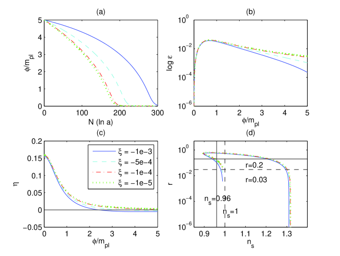
Figure 1: We plot (a) $\phi$ field evolution with the number of efolds $N$ (b) evolution of slow roll parameter $\epsilon$ with $\phi$, (c) evolution of slow-roll parameter $\eta$ with $\phi$, and (d) the spectral index of scalar perturbations $n_{s}$ versus tensor to scalar ratio $r$ with $\xi=-10^{-3},-5\times 10^{-4},-10^{-4}$ and $-10^{-5}$. We set $\lambda=g^{2}=1,v^{2}=10^{-4}m_{pl}^{2},\,\,m^{2}=10^{-8}m_{pl}^{2}$.

In the case of $\mu=0$, if $0<|\xi|<\frac{m^{2}}{\kappa^{2}\lambda v^{4}}$, the potential in the Einstein frame has a local maximum at $\phi=\phi_{e}$ which is given by

$$\phi=\phi_{e}:=\sqrt{\frac{m^{2}-\kappa^{2}|\xi|\lambda v^{4}}{\kappa^{2}|\xi|m^{2}}}.$$ (14)

and the potential at $\phi=\phi_{e}$ takes the value

$${\hat{V}}(\phi_{e},0)={\hat{V}}_{e}:=\frac{m^{4}}{4\kappa^{2}|\xi|\big{(}m^{2}-2|\xi|\kappa^{2}\lambda v^{4}\big{)}}.$$ (15)

In the small field region $\phi\gtrsim 0$, for $|\xi|<\frac{m^{2}}{\kappa^{2}\lambda v^{4}}$, $\frac{d\hat{V}}{d\hat{\phi}}>0$, and for $|\xi|>\frac{m^{2}}{\kappa^{2}\lambda v^{4}}$, $\frac{d\hat{V}}{d\hat{\phi}}<0$. In the latter case, since the potential does not contain the local minimum, there is no way to terminate the inflation. Thus, we will not consider the latter case in the present work.

For $|\xi|<\frac{m^{2}}{\kappa^{2}\lambda v^{4}}$, the slow-roll parameters are given by

$$\epsilon\simeq\frac{8(m^{2}-|\xi|\kappa^{2}\lambda v^{4})^{2}\phi^{2}}{\kappa^{2}\lambda^{2}v^{8}},\quad\eta\simeq\frac{8(m^{2}-|\xi|\kappa^{2}\lambda v^{4})}{\kappa^{2}\lambda v^{4}}>0.$$ (16)

Since as $\phi$ decreases $\epsilon$ decreases, inflation cannot be the type (II), but be the type (I), which is the ordinary hybrid inflation. The e-folding number is given by

$$N=\int_{{\hat{\phi}}_{f}}^{{\hat{\phi}}_{i}}\frac{\kappa^{2}{\hat{V}}}{{\hat{V}}_{,\hat{\phi}}}d\hat{\phi}=\int_{\phi_{f}}^{\phi_{i}}\frac{\kappa^{2}{\hat{V}}}{{\hat{V}}_{,\phi}}\Big{(}\frac{d\hat{\phi}}{d\phi}\Big{)}^{2}d\phi=\int_{\phi_{f}}^{\phi_{i}}\frac{\kappa d\phi}{\sqrt{2}\epsilon^{1/2}}\simeq\frac{\kappa^{2}\lambda v^{4}}{4(m^{2}-|\xi|\kappa^{2}\lambda v^{4})},$$ (17)

where $\phi_{i}$ and $\phi_{f}$ are the values at the beginning and the end of inflation, respectively, and we omit the logarithmic factor at the final expression. The slow-roll inflation can be realized for

$$0<\phi<\phi_{i}:=\frac{\kappa\lambda v^{4}}{2\sqrt{2}(m^{2}-\kappa^{2}|\xi|\lambda v^{4})},$$ (18)

where $\phi_{i}$ is determined from the condition that $\epsilon_{i}=1$. Since $N\simeq\frac{\kappa\phi_{i}}{\sqrt{2}}$, to obtain sufficiently long inflation, $\phi_{i}\gg\frac{1}{\kappa}$. Also, since $\phi_{e}>\phi_{i}$, we obtain $\phi_{e}\gg\frac{1}{\kappa}$, which leads to

$$|\xi|<\frac{m^{2}}{m^{2}+\kappa^{2}\lambda v^{4}}.$$

Then, we obtain

$$N<\frac{\kappa^{2}\lambda v^{4}}{4m^{2}}\Big{(}1+\frac{\kappa^{2}\lambda v^{4}}{m^{2}}\Big{)}.$$ (19)

The requirement $N>50$ gives $\frac{\kappa^{2}\lambda v^{4}}{m^{2}}\gtrsim 15$.

In this case, the amplitude of the curvature perturbations, the tensor-to-scalar ratio, and the spectral indices of the curvature and tensor perturbations are given by

$$P_{s} \simeq \frac{v^{12}\kappa^{6}\lambda^{3}}{768\pi^{2}\big{(}m^{2}-|\xi|\kappa^{2}\lambda v^{4}\big{)}^{2}\phi_{\ast}^{2}},\quad r\simeq\frac{128(m^{2}-|\xi|\kappa^{2}\lambda v^{4})^{2}\phi_{\ast}^{2}}{v^{8}\kappa^{2}\lambda^{2}},$$

$$n_{s}-1 \simeq 8\big{(}\frac{m^{2}}{\kappa^{2}\lambda v^{4}}-|\xi|\big{)}\simeq\frac{2}{N}>0,\quad n_{t}\simeq-\frac{16(m^{2}-|\xi|\kappa^{2}\lambda v^{4})^{2}\phi_{\ast}^{2}}{\kappa^{2}\lambda^{2}v^{8}}\,.$$ (20)

Thus, the spectrum is blue tilted.

In the region of $\phi>\phi_{e}$, there is no way to terminate inflation. Around the local maximum $\phi\lesssim\phi_{e}$, inflation can be either the type (I) or the type (II). For the tachyonic instability to appear, we need the condition $\phi_{e}>\phi>\phi_{c}$, which leads to

$$0<|\xi|<\frac{g^{2}m^{2}}{\kappa^{2}\lambda v^{2}(g^{2}v^{2}+m^{2})}.$$ (21)

The slow-roll parameters are given by

$$\epsilon \simeq \frac{32|\xi|^{2}\kappa^{2}m^{2}(m^{2}-|\xi|\kappa^{2}\lambda v^{4})^{2}(\phi-\phi_{e})^{2}}{(2m^{2}-\kappa^{2}\lambda v^{4})^{2}\big{[}m^{2}+(m^{2}-|\xi|\kappa^{2}\lambda v^{4})(1+6|\xi|)\big{]}},$$

$$\eta \simeq -\frac{8|\xi|(m^{2}-\kappa^{2}\lambda v^{4}|\xi|)}{m^{2}+(m^{2}-|\xi|\kappa^{2}\lambda v^{4})(1+6|\xi|)}<0.$$ (22)

The slow-roll condition is violated when $\epsilon=1$. The e-folding number is given by

$$N\simeq\frac{m^{2}+(m^{2}-|\xi|\kappa^{2}\lambda v^{4})(1+6|\xi|)}{8|\xi|(m^{2}-\kappa^{2}\lambda v^{4}|\xi|)}.$$ (23)

The amplitude of the curvature perturbations and the tensor-to-scalar ratio are given by

$$P_{s} \simeq \frac{(2m^{2}-\kappa^{2}|\xi|\lambda v^{4})\big{(}m^{2}+(m^{2}-|\xi|\kappa^{2}\lambda v^{4})(1+6|\xi|)\big{)}}{3072|\xi|^{3}\pi^{2}(m^{2}-|\xi|\kappa^{2}\lambda v^{4})(\phi_{\ast}-\phi_{e})^{2}},$$

$$r \simeq \frac{512\kappa^{2}m^{2}|\xi|^{2}(m^{2}-|\xi|\kappa^{2}\lambda v^{4})^{2}(\phi_{\ast}-\phi_{e})^{2}}{(2m^{2}-\kappa^{2}|\xi|\lambda v^{4})^{2}\big{(}m^{2}+(m^{2}-|\xi|\kappa^{2}\lambda v^{4})(1+6|\xi|)\big{)}},$$ (24)

respectively. The spectral index of the curvature perturbations is given by $n_{s}-1\simeq 2\eta\simeq-\frac{2}{N}<0$, namely red spectrum.

In order to follow the dynamics of the $\phi$ field from the local maximum to the vacuum dominated region, we perform the numerical calculations by solving the equations of motion. For the parameters $\lambda=g^{2}=1,\,\,v^{2}=10^{-4}\,m_{pl}^{2},\,\,m^{2}=10^{-8}\,m_{pl}^{2}$, we plot the evolution of the $\phi$ field, the evolution of the slow-roll parameters $\epsilon$ and $\eta$ and the relation between $n_{s}$ and $r$ in Fig. 1. We take into account $\phi_{i}$ being smaller than the local maximum $\phi_{e}$. In Fig. 1-(a), we find that enough number of e-folds can be obtained. The evolution of the slow-roll parameters are plotted in Figs. 1-(b) and 1-(c). Theses figures show that the slow-roll conditions are not violated, so inflation should be terminated through the tachyonic instability. We plot $n_{s}-r$ relation in Fig. 1-(d). The spectrum changes from red around the local maximum to blue in the vacuum dominated region.

III.2 The case of $m=0$

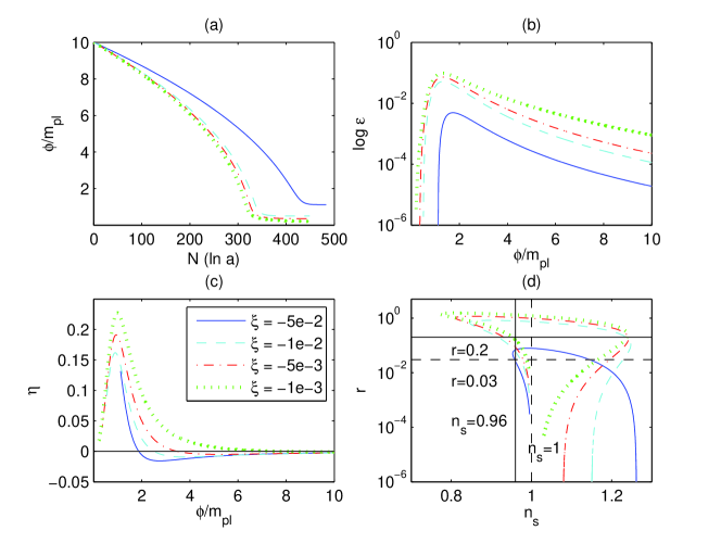
Figure 2: We plot (a) $\phi$ field evolution with the number of efolds $N$, (b) evolution of slow roll parameter $\epsilon$ with $\phi$, (c) evolution of slow-roll parameter $\eta$ with $\phi$ and (d) spectral index of scalar perturbations $n_{s}$ versus tensor to scalar ratio $r$ with $\xi=-5\times 10^{-2},-10^{-2},-5\times 10^{-3}$ and $-10^{-3}$. We set $\lambda=g^{2}=1,\,\,v^{2}=10^{-4}\,m_{pl}^{2},\,\,\mu=10^{-8}$.

In the case of $m=0$ but $\mu\neq 0$, along $\chi=0$ the potential has the local minima at $\phi=\phi_{e}$,

$$\phi=\phi_{e}:=\sqrt{\frac{\kappa^{2}\lambda v^{4}|\xi|}{\mu}},$$ (25)

and the potential at $\phi=\phi_{e}$ takes the nonzero minimum value

$${\hat{V}}(\phi_{e},0)={\hat{V}}_{e}:=\frac{v^{4}\lambda\mu}{4(\kappa^{4}\lambda v^{4}|\xi|^{2}+\mu)}.$$ (26)

Inflation can take place

(i) in the vacuum-dominated region,

(ii) around the local minimum,

(iii) in the large field inflation.

In the region (i), $\frac{d{\hat{V}}}{d\phi}\simeq-\kappa^{2}|\xi|\lambda v^{4}\phi<0$, and $\phi$ rolls down toward $\phi=\phi_{e}$. To obtain a stable potential, it must take place for $\phi>\phi_{c}$, where $\chi$ field has a positive mass. Then, inflation is the type (II). Around $\phi=0$, the slow-roll parameters become

$$\epsilon\simeq 8\kappa^{2}|\xi|^{2}\phi^{2},\quad\eta\simeq-4|\xi|.$$ (27)

Inflation is terminated when $\epsilon$ becomes order unity, namely at

$$\phi=\phi_{f}:=\frac{1}{2\sqrt{2}\kappa|\xi|}.$$ (28)

The e-folding number is given by

$$N\simeq\frac{1}{4|\xi|}\simeq\frac{\kappa\phi_{f}}{\sqrt{2}}.$$ (29)

Therefore, to get sufficiently long inflation, $\phi_{f}\gg\frac{1}{\kappa}$. On the other hand, since $\phi_{e}>\phi_{f}$, we have to require $\phi_{e}\gg\frac{1}{\kappa}$, which leads to $\frac{|\xi|}{\mu}>\frac{1}{\lambda\kappa^{4}v^{4}}$. Combining with (29), we obtain $N<\frac{\lambda\kappa^{4}v^{4}}{4\mu}$. We have to require $N>50$, and hence $\frac{\lambda\kappa^{4}v^{4}}{\mu}>200$. Recalling the sub-Planckian condition Eq. (10), unless $\mu\ll 1$, this condition cannot be satisfied. The amplitude of the curvature perturbations, the tensor-to-scalar ratio, and the spectral indices of the curvature and tensor perturbations are given by

$$P_{s} \simeq \frac{\kappa^{2}\lambda v^{4}}{768\pi^{2}|\xi|^{2}\phi_{\ast}^{2}},\quad r\simeq 128\kappa^{2}|\xi|^{2}\phi_{\ast}^{2},\quad n_{s}-1\simeq-8|\xi|<0,\quad n_{t}\simeq-16\kappa^{2}|\xi|^{2}\phi_{\ast}^{2},$$ (30)

respectively, where the field value $\phi_{\ast}$ is evaluated at the horizon crossing. The spectrum of the curvature perturbations is red tilted. In this case, however, since $V_{e}>0$, there is no way to terminate inflation in the original system.

In the region (ii) where $\phi$ field, located at $\phi>\phi_{e}$, begins to roll toward to $\phi_{e}$, inflation can be the type (I). The tachyonic instability appears at $\phi=\phi_{c}$, and we need to require $\phi_{c}>\phi_{e}$, or equivalently

$$|\xi|<\frac{\mu}{\kappa^{2}v^{2}g^{2}}.$$ (31)

Taking the sub-Planckian condition Eq. (10) into consideration, we can further restrict the range of the coupling. If $\mu^{\frac{1}{2}}<\frac{m^{2}}{\lambda v^{4}}$, then the type (I) inflation occurs for all the allowed region of Eq. (60). If $\mu^{\frac{1}{2}}<\frac{\mu}{\kappa^{2}v^{2}g^{2}}$, we obtain

$$\mu^{\frac{1}{2}}<|\xi|<\frac{\mu}{\kappa^{2}v^{2}g^{2}}.$$ (32)

If $\mu^{\frac{1}{2}}>\frac{\mu}{\kappa^{2}v^{2}g^{2}}$ there is no region where the type (I) inflation can occur at the sub-Planckian energy scale.

In the region (ii), assuming $\phi_{e}\lesssim\phi_{c}$, the slow-roll parameters

$$\epsilon \simeq \frac{32\kappa^{2}\mu^{3}|\xi|^{2}(\phi-\phi_{e})^{2}}{(\mu+|\xi|^{2}\kappa^{4}\lambda v^{4})^{2}\big{(}\mu+|\xi|^{2}\kappa^{4}\lambda v^{4}(1+6|\xi|)\big{)}},$$

$$\eta \simeq \frac{8|\xi|\mu}{\mu+|\xi|^{2}\kappa^{4}\lambda v^{4}(1+6|\xi|)}>0.$$ (33)

Note that as $\phi\to\phi_{e}$, $\epsilon$ becomes smaller, and there is no violation of the slow-roll conditions. Therefore, inflation must be the type (I). The e-folding number is given by

$$N \simeq \frac{\kappa^{4}|\xi|^{2}\lambda v^{4}\big{(}1+6|\xi|\big{)}+\mu}{8|\xi|\mu}.$$ (34)

The amplitude and spectral index of the curvature perturbations are given by

$$P_{s} \simeq \frac{v^{4}\kappa^{2}\lambda(|\xi|^{2}\kappa^{4}\lambda^{4}+\mu)(\mu+\kappa^{2}\lambda v^{4}|\xi|^{2}(1+6|\xi|))}{3072|\xi|^{2}\pi^{2}\mu^{2}(\phi_{\ast}-\phi_{e})^{2}},$$

$$n_{s}-1 \simeq \frac{16|\xi|\mu}{\mu+\kappa^{4}\lambda v^{4}|\xi|^{2}(1+6|\xi|)}\simeq\frac{2}{N},$$

$$n_{t} \simeq -\frac{64\kappa^{2}\mu^{3}|\xi|^{2}(\phi_{\ast}-\phi_{e})^{2}}{(\mu+|\xi|^{2}\kappa^{4}\lambda v^{4})^{2}\big{(}\mu+|\xi|^{2}\kappa^{4}\lambda v^{4}(1+6|\xi|)\big{)}}\simeq-2\epsilon,$$

$$r \simeq 16\epsilon.$$ (35)

The spectral index of the curvature perturbations is blue tilted.

In the region (iii), $\phi\gg\phi_{e}$, the slow-roll parameters Eq. (9) are given by

$$\epsilon\simeq\frac{8}{(1+6|\xi|)|\xi|\kappa^{4}\phi^{4}},\quad\eta\simeq-\frac{8}{(1+6|\xi|)\kappa^{2}\phi^{2}}<0,$$ (36)

and the slow-roll approximation is valid in the range

$$\phi>\phi_{f}=\frac{2\sqrt{2}}{(6|\xi|+1)^{\frac{1}{2}}\kappa}.$$ (37)

Inflation can be either the type (I) or the type (II). If $\phi_{c}>\phi_{f}$, inflation is the type (II), while if $\phi_{c}<\phi_{f}$ it is the type (I). The e-folding number from the horizon crossing to the end of inflation is given by

$$N\simeq\frac{(1+6|\xi|)\kappa^{2}\mu}{8\mu}\Big{(}\phi_{\ast}^{2}-\phi_{c,f}^{2}\Big{)}\simeq\frac{(1+6|\xi|)\kappa^{2}\phi_{\ast}^{2}}{8},$$ (38)

where we assume that $\phi_{\ast}\gg\phi_{c,f}$. The amplitude of the curvature perturbations and the tensor-to-scalar ratio are given by

$$P_{s}\simeq\frac{(1+6|\xi|)\kappa^{4}\mu\phi_{\ast}^{4}}{768|\xi|\pi^{2}},\quad r\simeq\frac{128}{|\xi|(1+6|\xi|)\kappa^{4}\phi_{\ast}^{4}}\simeq\frac{2}{N^{2}}\big{(}6+\frac{1}{|\xi|}\big{)}.$$ (39)

The spectral indices of the curvature and tensor perturbations become

$$n_{s}-1\simeq-\frac{16}{(1+6|\xi|)\kappa^{2}\phi_{\ast}^{2}}\simeq-\frac{2}{N}<0,$$

$$n_{t}\simeq-\frac{16}{(1+6|\xi|)|\xi|\kappa^{4}\phi_{\ast}^{4}}\simeq-\frac{1+6|\xi|}{4|\xi|N^{2}}<0.$$ (40)

Thus, the spectrum of the curvature perturbations is red tilted.

We perform the numerical calculations to track the evolution of $\phi$ field along $\chi=0$ and of slow-roll parameters $\epsilon$ and $\eta$ in Fig. 2. We set $\lambda=g^{2}=1,v^{2}=10^{-4}m_{pl}^{2}$ and $\mu=10^{-8}$ in Fig. 2. We find that the local minimum locates at $\phi=\phi_{e}$ in Fig. 2-(a). Given parameters for Fig. 2, as seen (33), slow-roll conditions are not violated (see Fig. 2-(b) and 2-(c)), so inflation should be terminated by the tachyonic instability. In order to terminate inflation by the tachyonic instability, it is necessary to satisfy the condition $\phi_{c}>\phi_{e}$. This condition leads to

$$|\xi|<|\xi_{c}|\equiv\frac{\mu}{\kappa^{2}v^{2}g^{2}}.$$ (41)

$|\xi_{c}|\sim 4\times 10^{-6}$ for the Fig. 2. In Fig. 2-(d) we plot $n_{s}-r$ relations. The figure shows that spectrum changes from red spectrum to blue ones.

III.3 $\phi^{2p}$ ($p>2$) model

Before closing this subsection, we briefly discuss the case of the potential in the Jordan frame given by

$$V(\phi,\chi)=\frac{1}{4}\lambda\big{(}\chi^{2}-v^{2}\big{)}^{2}+\frac{1}{2p}\mu\phi^{2p}+\frac{1}{2}g^{2}\phi^{2}\chi^{2},$$ (42)

where $p>2$ is an integer. Note that in this subsection $\mu$ parameter has mass dimension of $(-2(p-2))$, and in particular $(-4)$ for $p=3$. In this case, the potential in the Einstein frame $\hat{V}$ has a minimum at some $\phi=\phi_{e}>0$. For $p=3$, if $-1<\frac{A}{2\mu}<1$, where

$$A:=3|\xi|^{2}v^{4}\kappa^{6}\lambda-2\mu,$$ (43)

the extremal point is given by

$$\phi_{e}:=\frac{1}{\kappa|\xi|^{\frac{1}{2}}}\Big{(}-1+2\cos\big{(}\frac{x}{3}\big{)}\Big{)}^{\frac{1}{2}},$$ (44)

where $\cos x:=\frac{A}{2\mu}$. Note that $\frac{1}{2}<\cos\big{(}\frac{x}{3}\big{)}<1$. On the other hand, if $\frac{A}{2\mu}>1$, then it is given by

$$\phi_{e}:=\frac{1}{\kappa|\xi|^{\frac{1}{2}}}\Big{(}-1+2\cosh\big{(}\frac{y}{3}\big{)}\Big{)}^{\frac{1}{2}},$$ (45)

where $\cosh y:=\frac{A}{2\mu}$.

In the vacuum-dominated region, ${\hat{V}}$ is always negatively tilted. And thus inflation is the type (II) and is terminated at

$$\phi=\phi_{f}:=\frac{1}{2^{\frac{3}{2}}|\xi|\kappa}.$$ (46)

The typical e-folding number is given by

$$N\simeq\frac{1}{4|\xi|}\simeq\sqrt{2}\kappa\phi_{f}.$$ (47)

To realize sufficiently long inflation, we require $\phi_{f}>\frac{1}{\kappa}$, which leads to $|\xi|<1$ for $\frac{A}{2\mu}<1$ and $|\xi|<\frac{v^{4}\kappa^{6}\lambda}{\mu}$ for $\frac{A}{2\mu}>1$. Thus, we obtain $N>1$ for $\frac{A}{2\mu}<1$ and $N>\frac{\mu}{v^{4}\kappa^{6}\lambda}$ for $\frac{A}{2\mu}>1$.

Around the local minimum, it is naturally expected that the spectrum of the curvature perturbations produced inflation near $\phi=\phi_{e}$ is always blue tilted.

In the large field region, since $\frac{d{\hat{V}}}{d{\hat{\phi}}}>0$, $\phi$ is decreasing. The slow-roll parameters are given by

$$\epsilon \simeq \frac{2(p-2)^{2}|\xi|}{1+6|\xi|}+\frac{2(p-2)\big{(}(p+2)+12p|\xi|\big{)}}{\kappa^{2}(1+6|\xi|)^{2}\phi^{2}},$$

$$\eta \simeq \frac{4(p-2)^{2}|\xi|}{1+6|\xi|}+\frac{2(2p-5)\big{(}(p+2)+12p|\xi|\big{)}}{\kappa^{2}(1+6|\xi|)^{2}\phi^{2}}.$$ (48)

The slow-roll conditions is violated when $\epsilon$ or $\eta$ becomes $O(1)$ at

$$\phi\simeq\phi_{f}:=\frac{\sqrt{2(p-2)\big{(}(p+2)+12p|\xi|\big{)}}}{(1+6|\xi|)\kappa}.$$ (49)

For $\phi_{c}>\phi_{f}$, inflation is the type (I), and for $\phi_{c}<\phi_{f}$, it is the type (II). The e-folding number is given by

$$N\simeq\frac{1+6|\xi|}{2|\xi|(p-2)}.$$ (50)

The spectrum of the curvature perturbations, the tensor-to-scalar ratio, the spectral indices of the curvature and tensor perturbations are given by

$$P_{s}\simeq\frac{(1+6|\xi|)\mu\phi_{\ast}^{2(p-2)}}{96|\xi|^{3}(p-2)^{2}p\pi^{2}},\quad r\simeq\frac{32|\xi|(p-2)^{2}}{1+6|\xi|},$$

$$n_{s}-1\simeq-\frac{4(p-2)^{2}|\xi|}{1+6|\xi|}\simeq-\frac{2(p-2)}{N},\quad n_{t}\simeq-\frac{4(p-2)^{2}|\xi|}{1+6|\xi|}\simeq-\frac{2(p-2)}{N}.$$ (51)

Thus, the spectrum of the curvature perturbations is red tilted.

IV The case of $m\neq 0,\mu\neq 0$

In this section, we discuss inflationary dynamics in the Einstein frame in more details. Along $\chi=0$, the potential in the Einstein frame has the nonzero extremal value

$${\hat{V}}(\phi_{e},0)={\hat{V}}_{e}:=\frac{m^{4}-\mu\lambda v^{4}}{4\big{[}|\xi|\kappa^{2}m^{2}-\mu+|\xi|\kappa^{2}(m^{2}-|\xi|\kappa^{2}\lambda v^{4})\big{]}},$$ (52)

at

$$\phi=\phi_{e}:=\sqrt{\frac{-m^{2}-\kappa^{2}\lambda v^{4}\xi}{\mu+\kappa^{2}m^{2}\xi}}.$$ (53)

For $\frac{m^{4}}{\mu\lambda v^{4}}<1$, $\hat{V}_{e}$ becomes the minimum, while for $\frac{m^{4}}{\mu\lambda v^{4}}>1$, it becomes the maximum. For $\frac{m^{4}}{\mu\lambda v^{4}}=1$, the potential has no extremal point.

IV.1 $\frac{m^{4}}{\mu\lambda v^{4}}<1$

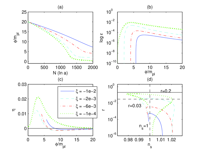
Figure 3: We plot (a) $\phi$ field evolution with the number of efolds $N$, (b) evolution of slow roll parameter $\epsilon$ with $\phi$, (c) evolution of slow-roll parameter $\eta$ with $\phi$, and (d) spectral index of scalar perturbations $n_{s}$ versus tensor to scalar ratio $r$ with $\xi=-10^{-2},-2\times 10^{-3},-6\times 10^{-3}$ and $-10^{-4}$. We set $\lambda=g^{2}=1,\,\,v^{2}=10^{-2}m_{pl}^{2},\,\,m^{2}=10^{-6}m_{pl}^{2},\,\,\mu=10^{-6}$. These parameter satisfy the condition $m^{4}<\mu\lambda v^{4}$ discussed in Sect. IV.1. While the potential is monotonically increasing for $\xi=-10^{-4}$, the potential has one local minimum at $\phi=\phi_{e}$ for $\xi=-10^{-2},-2\times 10^{-3}$ and $-6\times 10^{-3}$. As $|\xi|$ decreases, the local minimum shifts to the smaller $\phi$ and if $|\xi|\leq 3\times 10^{-4}$ the potential behaves as a monotonically increasing function of $\phi$.

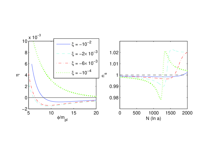
Figure 4: (left) Magnifying the Fig. 3-(c) in the region $5<\phi<20$. (right) evolution of spectral index $n_{s}$ of scalar perturbation.

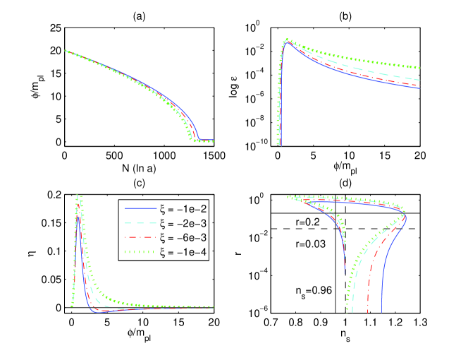
Figure 5: Same as Fig. 3 but we set $\lambda=g^{2}=1,\,\,v^{2}=10^{-2}\,m_{pl}^{2},\,\,m^{2}=10^{-6}\,m_{pl}^{2},\,\,\mu=10^{-4}$ which satisfy $m^{4}<\mu\lambda v^{4}$ (see Sect. IV.1) . For $\xi=-10^{-4}$, the potential is monotonically increasing. For $\xi=-10^{-2},-2\times 10^{-3}$ and $-6\times 10^{-3}$, the potential has one local minimum at $\phi=\phi_{e}$.

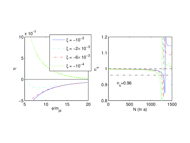
Figure 6: (left) Magnifying the Fig. 5-(c) in the region $5<\phi<20$. (right) evolution of spectral index $n_{s}$ of scalar perturbation.

In this case, in terms of the shape of $\hat{V}$, we separately discuss the following cases

(1) if $\frac{m^{2}}{\kappa^{2}\lambda v^{4}}<|\xi|<\frac{\mu}{\kappa^{2}m^{2}}$, there is one local minimum in the potential at $\phi=\phi_{e}$:

(2) if $\frac{m^{2}}{\kappa^{2}\lambda v^{4}}>|\xi|>0$, the potential is monotonically increasing:

(3) if $|\xi|>\frac{\mu}{\kappa^{2}m^{2}}$, the potential is monotonically decreasing:

(1):

In this case, there is the potential minimum at $\phi=\phi_{e}$. In the typical cases, inflation can take place

(i) in the vacuum-dominated region,

(ii) around the local minimum,

(iii) in the large field inflation.

In the region (i), $\frac{d{\hat{V}}}{d\phi}\simeq(m^{2}-\kappa^{2}|\xi|\lambda v^{4})\phi<0$, and $\phi$ rolls down toward $\phi=\phi_{e}$. To obtain a stable potential, it must take place for $\phi>\phi_{c}$. Then, inflation is the type (II). Around $\phi=0$, the slow-roll parameters become

$$\epsilon\simeq\frac{8(|\xi|\kappa^{2}\lambda v^{4}-m^{2})^{2}\phi^{2}}{v^{8}\kappa^{2}\lambda^{2}},\quad\eta\simeq-4(|\xi|-\frac{m^{2}}{v^{4}\kappa^{2}\lambda}).$$ (54)

Inflation is terminated where $\epsilon$ becomes order unity, namely at

$$\phi=\phi_{f}:=\frac{\kappa\lambda v^{4}}{2\sqrt{2}(|\xi|\kappa^{2}\lambda v^{4}-m^{2})}.$$ (55)

The e-folding number is given by

$$N\simeq\frac{\kappa^{2}\lambda v^{4}}{4(\kappa^{2}\lambda|\xi|v^{4}-m^{2})}\simeq\frac{\kappa\phi_{f}}{\sqrt{2}}.$$ (56)

Therefore, to get sufficiently long inflation, $\phi_{f}\gg\frac{1}{\kappa}$. On the other hand, we also require $\phi_{e}>\phi_{f}$, hence $\phi_{e}\gg\frac{1}{\kappa}$, which leads to

$$\frac{\mu}{\kappa^{2}m^{2}}>|\xi|>\frac{\kappa^{2}m^{2}+\mu}{\kappa^{2}m^{2}+\kappa^{2}\lambda v^{4}},$$

where the upper bound given from our classification. Combining with (56) we obtain

$$N<\frac{\kappa^{2}m^{2}+\kappa^{4}\lambda v^{4}}{4(\mu-\frac{m^{4}}{\lambda v^{4}})}.$$

We have to require $N>50$, hence

$$\frac{\kappa^{2}m^{2}+\kappa^{4}\lambda v^{4}}{\mu-\frac{m^{4}}{\lambda v^{4}}}>200.$$

For $\mu\gtrsim\frac{m^{4}}{\lambda v^{4}}$, this condition can be satisfied. In the limit of $m\to 0$, we recover the result in Sec. III-B.

The amplitude of the curvature perturbations, the tensor-to-scalar ratio, and the spectral indices of the curvature and tensor perturbations are given by

$$P_{s} \simeq \frac{v^{12}\kappa^{6}\lambda^{3}}{768\pi^{2}\big{(}m^{2}-|\xi|\kappa^{2}\lambda v^{4}\big{)}^{2}\phi_{\ast}^{2}},\quad r\simeq\frac{128(m^{2}-|\xi|\kappa^{2}\lambda v^{4})^{2}\phi_{\ast}^{2}}{v^{8}\kappa^{2}\lambda^{2}},$$

$$n_{s}-1 \simeq -8\big{(}|\xi|-\frac{m^{2}}{\kappa^{2}\lambda v^{4}}\big{)}<0,\quad n_{t}\simeq-\frac{16(m^{2}-|\xi|\kappa^{2}\lambda v^{4})^{2}\phi_{\ast}^{2}}{\kappa^{2}\lambda^{2}v^{8}}\,,$$ (57)

respectively, where the field value $\phi_{\ast}$ is evaluated at the horizon crossing. Thus, the spectrum of the curvature perturbations is red tilted.

In the two regions of (ii) and (iii), inflation can be the type (I). Let us clarify the conditions that the type (I) inflation takes place. The tachyonic instability appears at the place where $\chi$ deviates from $\chi=0$. Then, the critical field value must be greater than $\phi_{e}$, hence $\phi_{c}>\phi_{e}$, which leads to

$$|\xi|<|\xi_{c}|:=\frac{g^{2}m^{2}+\lambda\mu v^{2}}{\kappa^{2}\lambda v^{2}(m^{2}+g^{2}v^{2})}.$$ (58)

This is the generalization of Eq. (41) to the case of $m\neq 0$. Noting

$$\frac{\mu}{m^{2}}>|\xi_{c}|>\frac{m^{2}}{\lambda v^{4}},$$ (59)

the type (I) inflation can take place for

$$\frac{m^{2}}{\kappa^{2}\lambda v^{4}}<|\xi|<|\xi_{c}|.$$ (60)

Taking the sub-Planckian condition Eq. (10) into consideration, we can further restrict the range of the coupling. If $\mu^{\frac{1}{2}}<\frac{m^{2}}{\lambda v^{4}}$, then the type (I) inflation occurs for all the allowed region of Eq. (60). If $\frac{m^{2}}{\kappa^{2}\lambda v^{4}}<\mu^{\frac{1}{2}}<|\xi_{c}|$, we obtain

$$\mu^{\frac{1}{2}}<|\xi|<|\xi_{c}|.$$ (61)

If $\mu^{\frac{1}{2}}>|\xi_{c}|$, there is no region where the type (I) inflation can occur at the sub-Planckian energy scale.

In the region (ii), assuming $\phi_{e}\lesssim\phi_{c}$, the slow-roll parameters

$$\epsilon \simeq 32(|\xi|\kappa^{2}v^{4}\lambda-m^{2})^{2}(\mu-|\xi|\kappa^{2}m^{2})^{5}(\phi-\phi_{e})^{2}$$

$$\times \Big{\{}\kappa^{2}(\kappa^{2}m^{2}|\xi|-\mu+|\xi|\kappa^{2}(m^{2}-|\xi|\kappa^{2}v^{4}))^{2}$$

$$\times \big{[}(|\xi|\kappa^{2}v^{4}\lambda-m^{2})(1+6|\xi|)\kappa^{2}|\xi|+\mu-m^{2}\kappa^{2}|\xi|\big{]}(\lambda v^{4}\mu-m^{4})^{2}\Big{\}}^{-1}$$

$$\eta \simeq \frac{8(|\xi|\kappa^{2}\lambda v^{4}-m^{2})(\mu-|\xi|\kappa^{2}m^{2})^{2}}{\kappa^{2}\big{[}(|\xi|\kappa^{2}v^{4}\lambda-m^{2})(1+6|\xi|)\kappa^{2}|\xi|+\mu-m^{2}\kappa^{2}|\xi|\big{]}(\lambda v^{4}\mu-m^{4})}>0.$$ (62)

Note that as $\phi\to\phi_{e}$, $\epsilon$ becomes smaller, and there is no violation of the slow-roll conditions. Therefore, inflation must be the type (I). The e-folding number is given by

$$N \simeq \frac{\kappa^{2}\big{[}(|\xi|\kappa^{2}v^{4}-m^{2}\lambda)(1+6|\xi|)\kappa^{2}|\xi|+\mu-m^{2}\kappa^{2}|\xi|\big{]}(\lambda v^{4}\mu-m^{4})}{8(|\xi|\kappa^{2}\lambda v^{4}-m^{2})(\mu-|\xi|\kappa^{2}m^{2})^{2}}.$$ (63)

The amplitude and spectral index of the curvature perturbations are given by

$$P_{s} = \kappa^{6}\Big{[}(-2|\xi|\kappa^{2}m^{2}+|\xi|^{2}\kappa^{4}\lambda v^{4}+\mu)\big{(}-2|\xi|\kappa^{2}m^{2}+6|\xi|^{3}v^{4}\kappa^{4}\lambda+\kappa^{2}|\xi|(\kappa^{2}\lambda v^{4}-6m^{2})\big{)}$$

$$\times (m^{4}-\lambda\mu v^{4})^{3}\Big{]}$$

$$\times \Big{[}3072\pi^{2}(m^{2}-|\xi|\kappa^{2}\lambda v^{4})^{2}(|\xi\kappa^{2}m^{2}-\mu)^{5}(\phi_{\ast}-\phi_{e})^{2}\Big{]}^{-1},$$

$$n_{s}-1 \simeq \frac{16(|\xi|\kappa^{2}\lambda v^{4}-m^{2})(\mu-|\xi|\kappa^{2}m^{2})^{2}}{\kappa^{2}\big{[}(|\xi|\kappa^{2}v^{4}\lambda-m^{2})(1+6|\xi|)\kappa^{2}|\xi|+\mu-m^{2}\kappa^{2}|\xi|\big{]}(\lambda v^{4}\mu-m^{4})}\simeq\frac{2}{N}>0.$$ (64)

The spectral index of the curvature perturbations is blue tilted. The tensor spectral index and the tensor-to-scalar ratio are given by

$$n_{T}\simeq-2\epsilon,\quad r\simeq 16\epsilon.$$ (65)

In the region (iii), $\phi\gg\phi_{e}$, the slow-roll parameters Eq. (9) are given by

$$\epsilon\simeq\frac{8\big{(}\mu-|\xi|\kappa^{2}m^{2}\big{)}^{2}}{(1+6|\xi|)|\xi|\kappa^{4}\mu^{2}\phi^{4}},\quad\eta\simeq-\frac{8\big{(}\mu-|\xi|\kappa^{2}m^{2}\big{)}}{(1+6|\xi|)\kappa^{2}\mu\phi^{2}},$$ (66)

and the slow-roll approximation is valid in the range

$$\phi>\phi_{f}=\frac{2^{3/2}(\mu-|\xi|\kappa^{2}m^{2})^{1/2}}{(6|\xi|+1)^{1/2}(\kappa^{2}\mu)^{1/2}}.$$ (67)

Inflation can be either the type (I) or the type (I). If $\phi_{c}>\phi_{f}$, inflation is the type (II), while if $\phi_{c}<\phi_{f}$ it is the type (I). The e-folding number from the horizon crossing to the end of inflation is given by

$$N\simeq\frac{(1+6|\xi|)\kappa^{2}\mu}{8(\mu-|\xi|\kappa^{2}m^{2})}\Big{(}\phi_{\ast}^{2}-\phi_{c,f}^{2}\Big{)}\simeq\frac{(1+6|\xi|)\kappa^{2}\mu\phi_{\ast}^{2}}{8(\mu-|\xi|\kappa^{2}m^{2})},$$ (68)

where we assume that $\phi_{\ast}\gg\phi_{c,f}$. The amplitude of the curvature perturbations and the tensor-to-scalar ratio are given by

$$P_{s}\simeq\frac{(1+6|\xi|)\kappa^{4}\mu^{3}\phi_{\ast}^{4}}{768|\xi|\pi^{2}\big{(}\mu-|\xi|\kappa^{2}m^{2}\big{)}^{2}},\quad r\simeq\frac{128(\mu-|\xi|\kappa^{2}m^{2})^{2}}{|\xi|(1+6|\xi|)\kappa^{4}\mu^{2}\phi_{\ast}^{4}}\simeq\frac{2}{N^{2}}\big{(}6+\frac{1}{|\xi|}\big{)}.$$ (69)

The spectral indices of the curvature and tensor perturbations become

$$n_{s}-1\simeq-\frac{16\big{(}\mu-|\xi|\kappa^{2}m^{2}\big{)}}{(1+6|\xi|)\kappa^{2}\mu\phi_{\ast}^{2}}\simeq-\frac{2}{N}<0,$$

$$n_{t}\simeq-\frac{16\big{(}\mu-|\xi|\kappa^{2}m^{2}\big{)}^{2}}{(1+6|\xi|)|\xi|\kappa^{4}\mu^{2}\phi_{\ast}^{4}}\simeq-\frac{1+6|\xi|}{4|\xi|N^{2}}<0.$$ (70)

Thus, the spectrum of the curvature perturbations is red tilted.

(2):

The potential is monotonically increasing as $\phi$ increases, since $\phi_{e}\to 0$, as $\xi\to-\frac{m^{2}}{\kappa^{2}\lambda v^{4}}$ in the case (1). In this case, inflation can take place

(i) in the vacuum-dominated region

(ii) in the large field region

In the region (i), $\frac{d{\hat{V}}}{d\phi}\simeq(m^{2}-\kappa^{2}|\xi|\lambda v^{4})\phi>0$, and $\phi$ slowly rolls down toward the origin. Then, the slow-roll parameters are given by

$$\epsilon\simeq\frac{8(m^{2}-|\xi|\kappa^{2}\lambda v^{4})^{2}\phi^{2}}{\kappa^{2}\lambda^{2}v^{8}},\quad\eta\simeq\frac{4(m^{2}-|\xi|\kappa^{2}\lambda v^{4})}{\kappa^{2}\lambda v^{4}}>0.$$ (71)

Since $\epsilon$ is decreasing for decreasing $\phi$, inflation can be the type (I). The e-folding number is given by

$$N\simeq\frac{\kappa^{2}\lambda v^{4}}{4(m^{2}-\kappa^{2}\lambda|\xi|v^{4})}.$$ (72)

The slow-roll inflation can be realized for

$$0<\phi<\phi_{i}:=\frac{\kappa\lambda v^{4}}{2\sqrt{2}(-|\xi|\kappa^{2}\lambda v^{4}+m^{2})},$$ (73)

where $\epsilon_{i}=1$. Noting that $N\simeq\frac{\kappa\phi_{i}}{\sqrt{2}}$, to realize sufficiently long inflation, $\phi_{i}\gg\frac{1}{\kappa}$, which gives

$$\frac{m^{2}}{\kappa^{2}\lambda v^{4}}>|\xi|>\frac{m^{2}}{\kappa^{2}\lambda v^{4}}-\frac{1}{2\sqrt{2}}$$

(if $\frac{m^{2}}{\kappa^{2}\lambda v^{4}}>\frac{1}{2\sqrt{2}}$), where the upper bound is given from our classifications.

The amplitude of the curvature perturbations, the tensor-to-scalar ratio, and the spectral indices of the curvature and tensor perturbations are given by

$$P_{s} \simeq \frac{v^{12}\kappa^{6}\lambda^{3}}{768\pi^{2}\big{(}m^{2}-|\xi|\kappa^{2}\lambda v^{4}\big{)}^{2}\phi_{\ast}^{2}},\quad r\simeq\frac{128(m^{2}-|\xi|\kappa^{2}\lambda v^{4})^{2}\phi_{\ast}^{2}}{v^{8}\kappa^{2}\lambda^{2}},$$

$$n_{s}-1 \simeq 8\big{(}\frac{m^{2}}{\kappa^{2}\lambda v^{4}}-|\xi|\big{)}>0,\quad n_{t}\simeq-\frac{16(m^{2}-|\xi|\kappa^{2}\lambda v^{4})^{2}}{\kappa^{2}\lambda^{2}v^{8}}\,.$$ (74)

Thus, the spectrum of the curvature perturbations is blue tilted.

In the region (ii), the background dynamics and predictions can be written as the same manner as those in (1)-(iii). We now discuss the condition that inflation takes place at the sub-Planckian scale. If $\mu^{\frac{1}{2}}<\frac{m^{2}}{\kappa^{2}\lambda v^{4}}$, then inflation takes place at a sub-Planckian energy scale for

$$\mu^{\frac{1}{2}}<|\xi|<\frac{m^{2}}{\kappa^{2}\lambda v^{4}}.$$ (75)

For $\mu^{\frac{1}{2}}>\frac{m^{2}}{\kappa^{2}\lambda v^{4}}$, there is no region where inflation can occur in the sub-Planckian energy scale.

Until now we have discussed inflation realized in each typical region. In these cases, in general $\phi$ field moves from the large field region toward the local minimum or to the vacuum dominated region. To follow the whole dynamics, we need to solve the equations of motion numerically.

In Fig. 3 and 5, we plot $\phi$ field evolution with the number of e-folds $N$ in panel (a), evolution of slow-roll parameters $\epsilon$ and $\eta$ in panel (b) and (c), and the relation between the spectral index of scalar perturbations $n_{s}$ and the tensor to scalar ratio $r$ in panel (d) with $\xi=-10^{-2},-2\times 10^{-3},-6\times 10^{-3}$ and $-10^{-4}$. We set the parameters to $\lambda=1,\,\,g^{2}=1,\,\,v^{2}=10^{-2}\,m_{pl}^{2},\,\,m^{2}=10^{-6}\,m_{pl}^{2},\,\,\mu=10^{-6}$ for Fig. 3 and to $\lambda=1,\,\,g^{2}=1,\,\,v^{2}=10^{-2}\,m_{pl}^{2},\,\,m^{2}=10^{-6}\,m_{pl}^{2},\,\,\mu=10^{-4}$ for Fig. 5. Both parameter set satisfy the condition $m^{4}<\mu\lambda v^{4}$. In Fig. 3, we find that as $|\xi|$ decreases, the local minimum value $\phi_{e}$ shifts to smaller $\phi$. For $\xi=-10^{-4}$, the potential increases monotonically ($\phi_{e}=0$). If $|\xi|<\frac{m^{2}}{\kappa^{2}\lambda v^{4}}\simeq 4\times 10^{-4}$, the potential behaves as an increasing function of $\phi$. If $|\xi|\geq\frac{m^{2}}{\kappa^{2}\lambda v^{4}}\simeq 4\times 10^{-4}$, there exists a local maximum at $\phi=\phi_{e}$. On the other hand, if $|\xi|\geq\frac{\mu}{\kappa^{2}m^{2}}\simeq 4\times 10^{-2}$, the potential decreases monotonically as $\phi$ increases which will discuss below. We find in Fig. 3-(a) the $\phi$ field reach to $\phi_{e}$ after slow-rolling over potential during inflation period.

Fig. 3-(b) and 3-(c) show the evolution of the slow-roll parameters $\epsilon$ and $\eta$. These figures show that slow-roll conditions are not violated for the chosen parameter, so inflation should be terminated by the tachyonic instability. We find in Fig. 3-(c) that the slow-roll parameter $\eta$ has positive values for $\xi=-10^{-4}$ and have negative values for $\xi=-10^{-2},2\times 10^{-3}$ and $6\times 10^{-3}$ during slow-roll phase. We plot the slow-roll parameter $\eta$ in detail during slow-roll phase in Fig. 4-(left). These imply that the potential have positive curvature ($\xi=-10^{-4}$) or negative curvature ($\xi=-10^{-2},2\times 10^{-3},6\times 10^{-3}$) during inflation.

Fig. 3-(d) shows the relation between the spectral index $n_{s}$ and the tensor to scalar ratio $r$. In order to compare with the observations, we draw the bound $r=0.2$ (horizontal black solid line) from WMAP satellite and $r=0.03$ (horizontal black dashed line) from PLANCK satellite Efstathiou:2009xv . Since $n_{s}=0.968\pm 0.012$ from WMAP data Komatsu:2010fb , Fig. 3-(d) indicates that $n_{s}$ is well fit to the data in $2\sigma\,(95\%CL)$. We find from Fig. 4-(right) that the spectral index shows the red spectrum in the large field region and then moves to the blue spectrum around the local minimum.

In Fig. 5, the potential shows similar behavior as in Fig. (3) except that for $|\xi|\geq\frac{\mu}{\kappa^{2}m^{2}}\simeq 4$ the potential decreases monotonically as $\phi$ increases. Fig. 5-(c) shows the evolution of the slow-roll parameter $\eta$ and we can look at more closely the behavior of $\eta$ during slow-roll phase in Fig. 6-(left).

The relation between the spectral index $n_{s}$ and the tensor to scalar ratio $r$ are shown in Fig. 5-(d) and the evolution of $n_{s}$ are plotted in Fig. 6-(right). The best fit of $n_{s}$ from WMAP ($n_{s}=0.96$) as well as $r=0.2$ and $r=0.03$ are drawn in Fig. 5-(d). Like as in Fig. 3, the figure shows the spectrum moves from red spectrum to blue ones.

(3):

The potential is monotonically decreasing as $\phi$ becomes larger, since $\phi_{e}\to\infty$, as $\xi\to-\frac{\mu}{\kappa^{2}m^{2}}$ in the subcase (1). In this case, there is no way to realize the reheating, since the tachyonic instability does not occur. Thus, in this paper we do not consider this case.

IV.2 $\frac{m^{4}}{\mu\lambda v^{4}}>1$

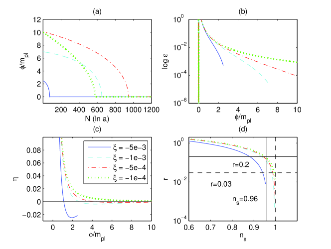
Figure 7: We plot (a) $\phi$ field evolution with the number of efolds, $N$, (b) evolution of slow roll parameter $\epsilon$ with $\phi$, (c) evolution of slow-roll parameter $\eta$ with $\phi$, and (d) spectral index of scalar perturbations $n_{s}$ versus tensor to scalar ratio $r$ with $\xi=-5\times 10^{-3},-10^{-3},-5\times 10^{-4}$ and $-10^{-4}$. We set $\lambda=g^{2}=1,v^{2}=10^{-2}m_{pl}^{2},m^{2}=10^{-2}m_{pl}^{2},\mu=10^{-4}$. These parameter satisfy the condition $m^{4}>\mu\lambda v^{4}$ discussed in Sect. IV.2. For $\xi=-10^{-4}$, the potential is monotonically increasing. The potential has one local maxima for $\xi=-5\times 10^{-3},-10^{-3}$ and $-5\times 10^{-4}$. The local maxima shift to the right as $|\xi|$ decreases. If $|\xi|>5$, the potential is monotonically decreasing but we do not plot for this case.

Similarly, we discuss the following three cases separately

(1) if $\frac{\mu}{\kappa^{2}m^{2}}<|\xi|<\frac{m^{2}}{\kappa^{2}\lambda v^{4}}$, there is one local maximum at $\phi=\phi_{e}$:

(2) if $\frac{\mu}{\kappa^{2}m^{2}}>|\xi|>0$, the potential is monotonically increasing:

(3) if $|\xi|>\frac{m^{2}}{\kappa^{2}\lambda v^{4}}$, the potential is monotonically decreasing:

(1):

In this case, there is a local maximum in the potential. Then inflation can take place

(i) in the vacuum-dominated region where ${\hat{V}}_{,\phi}>0$

(ii) around the local maximum

(iii) in the large field region

In the region (i), $\frac{d{\hat{V}}}{d\phi}\simeq(m^{2}-\kappa^{2}|\xi|\lambda v^{4})\phi>0$. Thus, $\phi$ rolls down toward the origin. Then, the slow-roll parameters and the e-folding number are given by Eq. (16) and Eq. (17). By the same reasoning from Sect. III.1 inflation must be the type (I). The slow-roll inflation can be realized for

$$0<\phi<\phi_{i}:=\frac{\kappa\lambda v^{4}}{2\sqrt{2}(m^{2}-|\xi|\kappa^{2}\lambda v^{4})},$$ (76)

where $\epsilon_{i}=1$. Noting that $N\simeq\frac{\kappa\phi_{i}}{\sqrt{2}}$, in order to realize sufficiently long inflation, $\phi_{i}\gg\frac{1}{\kappa}$. On the other hand, we also need to require $\phi_{e}>\phi_{i}$, hence $\phi_{e}\gg\frac{1}{\kappa}$, which leads to

$$\frac{m^{2}}{\kappa^{2}\lambda v^{4}}>|\xi|>\frac{\kappa^{2}m^{2}+\mu}{\kappa^{2}m^{2}+\kappa^{4}\lambda v^{4}},$$

where the upper bound is given from our classification. Combining with (17), we obtain

$$N<\frac{\kappa^{2}m^{2}+\kappa^{4}\lambda v^{4}}{4(\frac{m^{4}}{\lambda v^{4}}-\mu)}.$$

We have to require $N>50$, hence

$$\frac{\kappa^{2}m^{2}+\kappa^{4}\lambda v^{4}}{\frac{m^{4}}{\lambda v^{4}}-\mu}>200.$$

For $\mu\lesssim\frac{m^{4}}{\lambda v^{4}}$, this condition can be satisfied.

The amplitude of the curvature perturbations, the tensor-to-scalar ratio, and the spectral indices of the curvature and tensor perturbations are given by

$$P_{s} \simeq \frac{v^{12}\kappa^{6}\lambda^{3}}{768\pi^{2}\big{(}m^{2}-|\xi|\kappa^{2}\lambda v^{4}\big{)}^{2}\phi_{\ast}^{2}},\quad r\simeq\frac{128(m^{2}-|\xi|\kappa^{2}\lambda v^{4})^{2}\phi_{\ast}^{2}}{v^{8}\kappa^{2}\lambda^{2}},$$

$$n_{s}-1 \simeq 8\big{(}\frac{m^{2}}{\kappa^{2}\lambda v^{4}}-|\xi|\big{)}>0,\quad n_{t}\simeq-\frac{16(m^{2}-|\xi|\kappa^{2}\lambda v^{4})^{2}\phi_{\ast}^{2}}{\kappa^{2}\lambda^{2}v^{8}}\,.$$ (77)

Thus, the spectrum of the curvature perturbations is blue tilted.

In the region (ii), around the local maximum, the slow-roll parameters are given by

$$\epsilon \simeq 32(m^{2}-|\xi|\kappa^{2}v^{4}\lambda)^{2}(|\xi|\kappa^{2}m^{2}-\mu)^{5}(\phi-\phi_{e})^{2}$$

$$\times \Big{\{}\kappa^{2}(\kappa^{2}m^{2}|\xi|-\mu+|\xi|\kappa^{2}(m^{2}-|\xi|\kappa^{2}v^{4}))^{2}$$

$$\times \big{[}(m^{2}-|\xi|\kappa^{2}v^{4}\lambda)(1+6|\xi|)\kappa^{2}|\xi|+m^{2}\kappa^{2}|\xi|-\mu\big{]}(m^{4}-\lambda v^{4}\mu)^{2}\Big{\}}^{-1}$$

$$\eta \simeq -\frac{8(m^{2}-|\xi|\kappa^{2}\lambda v^{4})(\mu-|\xi|\kappa^{2}m^{2})^{2}}{\kappa^{2}\big{[}(m^{2}-|\xi|\kappa^{2}v^{4}\lambda)(1+6|\xi|)\kappa^{2}|\xi|+m^{2}\kappa^{2}|\xi|-\mu\big{]}(m^{4}-\lambda v^{4}\mu)}<0.$$ (78)

For $\phi<\phi_{e}$, inflation can be either the type (I) or the type (II). For $\phi>\phi_{e}$, it can be only the type (II). The e-folding number is given by

$$N \simeq \frac{\kappa^{2}\big{[}(m^{2}-|\xi|\kappa^{2}v^{4}\lambda)(1+6|\xi|)\kappa^{2}|\xi|+m^{2}\kappa^{2}|\xi|-\mu\big{]}(m^{4}-\lambda v^{4}\mu)}{8(m^{2}-|\xi|\kappa^{2}\lambda v^{4})(\mu-|\xi|\kappa^{2}m^{2})^{2}}.$$ (79)

The spectral index of the curvature perturbations is given by

$$n_{s}-1\simeq-\frac{16(m^{2}-|\xi|\kappa^{2}\lambda v^{4})(\mu-|\xi|\kappa^{2}m^{2})^{2}}{\kappa^{2}\big{[}(m^{2}-|\xi|\kappa^{2}v^{4}\lambda)(1+6|\xi|)\kappa^{2}|\xi|m^{2}\kappa^{2}|\xi|-\mu\big{]}(m^{4}-\lambda v^{4}\mu)}\simeq-\frac{2}{N}.$$ (80)

The tensor spectral index and the tensor-to-scalar ratio are given by $n_{t}\simeq-2\epsilon$ and $r\simeq 16\epsilon$.

In the region (iii), inflation can not be the type (I). In addition, as $\phi$ increases the slow-roll parameters

$$\epsilon\simeq\frac{8(|\xi|\kappa^{2}m^{2}-\mu)^{2}}{(1+6|\xi|)|\xi|\kappa^{4}\mu^{2}\phi^{4}},\quad\eta\simeq\frac{8(|\xi|\kappa^{2}m^{2}-\mu)}{(1+6|\xi|)\kappa^{2}\mu\phi^{2}},$$ (81)

decrease. Therefore there is no way to terminate inflation.

(2):

The potential is monotonically increasing as $\phi$ becomes larger, since $\phi_{e}\to\infty$ as $\xi\to-\frac{\mu}{\kappa^{2}m^{2}}$ in the subcase (1). The inflation can take place

(i) in the vacuum-dominated region

(ii) in the large field region

In the region (i), $\frac{d{\hat{V}}}{d\phi}\simeq(m^{2}-\kappa^{2}|\xi|\lambda v^{4})\phi>0$. Thus, $\phi$ rolls down toward $\phi=0$. Then, the slow-roll parameters are given by

$$\epsilon\simeq\frac{8(m^{2}-|\xi|\kappa^{2}\lambda v^{4})^{2}\phi^{2}}{\kappa^{2}\lambda^{2}v^{8}},\quad\eta\simeq\frac{8(m^{2}-|\xi|\kappa^{2}\lambda v^{4})}{\kappa^{2}\lambda v^{4}}>0.$$ (82)

Since as $\phi$ decreases $\epsilon$ decreases, inflation cannot be the type (II), but be the type (I). The e-folding number is given by

$$N\simeq\frac{\kappa^{2}\lambda v^{4}}{4(m^{2}-\kappa^{2}\lambda|\xi|v^{4})}.$$ (83)

The slow-roll inflation can be realized for

$$0<\phi<\phi_{i}:=\frac{\kappa\lambda v^{4}}{2\sqrt{2}(m^{2}-|\xi|\kappa^{2}\lambda v^{4})},$$ (84)

where $\epsilon_{i}=1$. Noting that $N\simeq\frac{\kappa\phi_{i}}{\sqrt{2}}$, to realize sufficiently long inflation, $\phi_{i}\gg\frac{1}{\kappa}$, which leads to

$$\frac{\mu}{\kappa^{2}m^{2}}>|\xi|>\frac{m^{2}}{\kappa^{2}\lambda v^{4}}-\frac{1}{2\sqrt{2}},$$

where the upper bound is given from our classifications.

The amplitude of the curvature perturbations, the tensor-to-scalar ratio, and the spectral indices of the curvature and tensor perturbations are given by

$$P_{s} \simeq \frac{v^{12}\kappa^{6}\lambda^{3}}{768\pi^{2}\big{(}m^{2}-|\xi|\kappa^{2}\lambda v^{4}\big{)}^{2}\phi_{\ast}^{2}},\quad r\simeq\frac{128(m^{2}-|\xi|\kappa^{2}\lambda v^{4})^{2}\phi_{\ast}^{2}}{v^{8}\kappa^{2}\lambda^{2}},$$

$$n_{s}-1 \simeq 8\big{(}\frac{m^{2}}{\kappa^{2}\lambda v^{4}}-|\xi|\big{)}>0,\quad n_{t}\simeq-\frac{16(m^{2}-|\xi|\kappa^{2}\lambda v^{4})^{2}\phi_{\ast}^{2}}{\kappa^{2}\lambda^{2}v^{8}}\,.$$ (85)

Thus, the spectrum of the curvature perturbations is blue tilted.

In the region (ii), $\phi\gg\phi_{e}$, the slow-roll parameters Eq. (9) are given by

$$\epsilon\simeq\frac{8\big{(}\mu-|\xi|\kappa^{2}m^{2}\big{)}^{2}}{(1+6|\xi|)|\xi|\kappa^{4}\mu^{2}\phi^{4}},\quad\eta\simeq-\frac{8\big{(}\mu-|\xi|\kappa^{2}m^{2}\big{)}}{(1+6|\xi|)\kappa^{2}\mu\phi^{2}},$$ (86)

and the slow-roll approximation is valid in the range

$$\phi>\phi_{f}=\frac{2^{3/2}(\mu-|\xi|\kappa^{2}m^{2})^{1/2}}{(6|\xi|+1)^{1/2}(\kappa^{2}\mu)^{1/2}}.$$ (87)

Inflation can be either the type (I) or the type (I). If $\phi_{c}>\phi_{f}$, inflation is the type (I), while if $\phi_{c}<\phi_{f}$ it is the type (II). The e-folding number from the horizon crossing to the end of inflation is given by

$$N\simeq\frac{(1+6|\xi|)\kappa^{2}\mu}{8(\mu-|\xi|\kappa^{2}m^{2})}\Big{(}\phi_{\ast}^{2}-\phi_{c,f}^{2}\Big{)}\simeq\frac{(1+6|\xi|)\kappa^{2}\mu\phi_{\ast}^{2}}{8(\mu-|\xi|\kappa^{2}m^{2})},$$ (88)

where we assume that $\phi_{\ast}\gg\phi_{c,f}$. The amplitude of the curvature perturbations and the tensor-to-scalar ratio are given by

$$P_{s}\simeq\frac{(1+6|\xi|)\kappa^{4}\mu^{3}\phi_{\ast}^{4}}{768|\xi|\pi^{2}\big{(}\mu-|\xi|\kappa^{2}m^{2}\big{)}^{2}},\quad r\simeq\frac{128(\mu-|\xi|\kappa^{2}m^{2})^{2}}{|\xi|(1+6|\xi|)\kappa^{4}\mu^{2}\phi_{\ast}^{4}}\simeq\frac{2}{N^{2}}\big{(}6+\frac{1}{|\xi|}\big{)}.$$ (89)

The spectral indices of the curvature and tensor perturbations become

$$n_{s}-1\simeq-\frac{16\big{(}\mu-|\xi|\kappa^{2}m^{2}\big{)}}{(1+6|\xi|)\kappa^{2}\mu\phi_{\ast}^{2}}\simeq-\frac{2}{N}<0,$$

$$n_{t}\simeq-\frac{16\big{(}\mu-|\xi|\kappa^{2}m^{2}\big{)}^{2}}{(1+6|\xi|)|\xi|\kappa^{4}\mu^{2}\phi_{\ast}^{4}}\simeq-\frac{1+6|\xi|}{4|\xi|N^{2}}<0.$$ (90)

Thus, the spectrum of the curvature perturbations is red tilted.

We perform the numerical calculations to follow the whole dynamics from the local maximum to the vacuum-dominated region. We consider the cases of $\xi=-5\times 10^{-3},\,\,-10^{-3},\,\,-5\times 10^{-4}$ and $-10^{-4}$ with the parameters $\lambda=1,\,\,g^{2}=1,\,\,v^{2}=10^{-2}m_{pl}^{2},\,\,m^{2}=10^{-2}m_{pl}^{2},\,\,\mu=10^{-4}$ in Fig. 7 in order to compute the $\phi$ field evolutions, evolution of slow-roll parameters $\epsilon$ and $\eta$, and the behavior of the spectral index of the scalar perturbation $n_{s}$ and the tensor to scalar ratio $r$. Since the chosen parameter set satisfy the condition $m^{4}>\mu\lambda v^{4}$, the potential either has a local maxima at $\phi=\phi_{e}$ or increases as $\phi$ increases. If $|\xi|<\frac{\mu}{\kappa^{2}m^{2}}\simeq 4\times 10^{-4}$, the potential increases monotonically as $\phi$ increases ($\phi_{e}=\infty$). If $|\xi|\geq\frac{\mu}{\kappa^{2}m^{2}}\simeq 4\times 10^{-4}$, the local maximum locates at $\phi_{e}$. We find that as $|\xi|$ increases, the local maximum shifts to the smaller $\phi$. This implies that if $|\xi|\geq\frac{m^{2}}{\kappa^{2}\lambda v^{4}}\simeq 4$, the potential becomes monotonically decreasing function of $\phi$ which will be discussed below. We choose the initial value of $\phi$ in the region $\phi_{i}<\phi_{e}$ where the $\phi$ field rolls toward to origin (see Fig. 7-(a)).

Figs. 7-(b) and 7-(c) show the evolution of the slow-roll parameters $\epsilon$ and $\eta$. Since the slow-roll conditions are not violated, inflation should be terminated by the tachyonic instability. Fig. 7-(c) shows negative $\eta$ (negative curvature potential) for $\xi=-5\times 10^{-3},\,\,-10^{-3},\,\,-5\times 10^{-4}$ and positive $\eta$ (positive curvature potential) for $\xi=-10^{-4}$ during slow-roll phase. We plot $n_{s}-r$ relation in Fig. 7-(d). Unlike the case in Sect. IV.1, the spectrum do not cross to the blue spectrum region ($n_{s}<1$) even after the slow-roll phase.

(3):

The potential is monotonically decreasing as $\phi$ becomes larger, since $\phi_{e}\to 0$, as $\xi\to-\frac{m^{2}}{\kappa^{2}\lambda v^{4}}$ in the subcase (1). In this case, there is no way to realize the reheating, since the tachyonic instability does not take place. Thus, in this paper we do not consider this case.

IV.3 $\frac{m^{4}}{\mu\lambda v^{4}}=1$

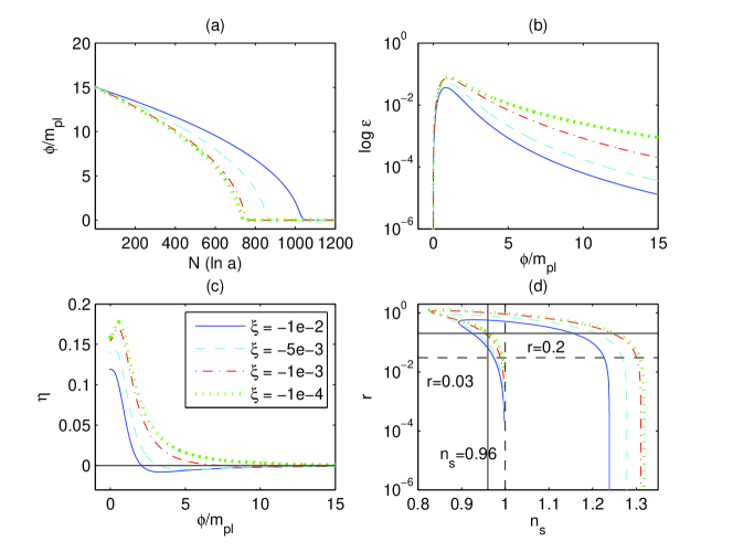
Figure 8: We plot same figures as in Fig. 3 with $\lambda=g^{2}=1,v^{2}=10^{-2}m_{pl}^{2},m^{2}=10^{-4}m_{pl}^{2},\mu=10^{-4}$ and this parameter satisfy $m^{4}=\mu\lambda v^{4}$ (see Sect. IV.3). For these parameter range, the potential behaves monotonically increasing or decreasing function of $\phi$. While the potential decreases as $\phi$ increases for $|\xi|\geq 4\times 10^{-2}$, the potential is monotonically increasing as $\phi$ increases for $|\xi|<4\times 10^{-2}$

Figure 9: Magnifying the Fig. 8-(c) in the region $5<\phi<15$. (right) evolution of spectral index $n_{s}$ of scalar perturbation.

In this case, along $\chi=0$

$${\hat{V}}=\frac{(\lambda v^{4}+m^{2}\phi^{2})^{2}}{4\lambda v^{4}\big{(}1+|\xi|\kappa^{2}\phi^{2}\big{)}^{2}},$$ (91)

and therefore, the potential is the monotonic for $\phi$. Since

$$\frac{d{\hat{V}}}{d\phi}=\frac{(m^{2}-|\xi|\kappa^{4}\lambda v^{4})\phi(\lambda v^{4}+m^{2}\phi^{2})}{\lambda v^{4}(1+|\xi|\kappa^{2}\phi^{2})^{3}},$$

for $|\xi|<\frac{m^{2}}{\kappa^{2}v^{4}\lambda}$, the potential is increasing, while for $|\xi|>\frac{m^{2}}{\kappa^{2}v^{4}\lambda}$, it is decreasing.

IV.3.1 $0<|\xi|<\frac{m^{2}}{\kappa^{2}v^{4}\lambda}$

Inflation can take place

(i) in the vacuum-dominated region

(ii) in the large field region

In the region (i), the slow-roll parameters are given by

$$\epsilon\simeq\frac{8(m^{2}-|\xi|\kappa^{2}\lambda v^{4})^{2}\phi^{2}}{\kappa^{2}\lambda^{2}v^{8}},\quad\eta\simeq\frac{4(m^{2}-|\xi|\kappa^{2}\lambda v^{4})}{\kappa^{2}\lambda v^{4}}>0.$$ (92)

Since $\epsilon$ is decreasing for decreasing $\phi$, inflation cannot be the type (II), but the type (I). The e-folding number is given by

$$N\simeq\frac{\kappa^{2}\lambda v^{4}}{4(m^{2}-\kappa^{2}\lambda|\xi|v^{4})}.$$ (93)

The slow-roll inflation can be realized for

$$0<\phi<\phi_{i}:=\frac{\kappa\lambda v^{4}}{2\sqrt{2}(-|\xi|\kappa^{2}\lambda v^{4}+m^{2})},$$ (94)

where $\epsilon_{i}=1$. Noting that $N\simeq\frac{\kappa\phi_{i}}{\sqrt{2}}$, to realize sufficiently long inflation, $\phi_{i}\gg\frac{1}{\kappa}$, which leads to

$$\frac{m^{2}}{\kappa^{2}\lambda v^{4}}>|\xi|>\frac{m^{2}}{\kappa^{2}\lambda v^{4}}-\frac{1}{2\sqrt{2}}$$

(if $\frac{m^{2}}{\kappa^{2}\lambda v^{4}}>\frac{1}{2\sqrt{2}}$), where the upper bound is given from our classifications.

The amplitude of the curvature perturbations, the tensor-to-scalar ratio, and the spectral indices of the curvature and tensor perturbations are given by

$$P_{s} \simeq \frac{v^{12}\kappa^{6}\lambda^{3}}{768\pi^{2}\big{(}m^{2}-|\xi|\kappa^{2}\lambda v^{4}\big{)}^{2}\phi_{\ast}^{2}},\quad r\simeq\frac{128(m^{2}-|\xi|\kappa^{2}\lambda v^{4})^{2}\phi_{\ast}^{2}}{v^{8}\kappa^{2}\lambda^{2}},$$

$$n_{s}-1 \simeq 8\big{(}\frac{m^{2}}{\kappa^{2}\lambda v^{4}}-|\xi|\big{)}>0,\quad n_{t}\simeq-\frac{16(m^{2}-|\xi|\kappa^{2}\lambda v^{4})^{2}\phi_{\ast}^{2}}{\kappa^{2}\lambda^{2}v^{8}}\,.$$ (95)

Thus, the spectrum of the curvature perturbations is blue tilted.

In the region (ii), the slow-roll parameters are given by

$$\epsilon\simeq\frac{8\big{(}m^{2}-|\xi|\kappa^{2}\lambda v^{4}\big{)}^{2}}{(1+6|\xi|)|\xi|m^{4}\kappa^{4}\phi^{4}},\quad\eta\simeq-\frac{8\big{(}m^{2}-|\xi|\kappa^{2}\lambda v^{4}\big{)}}{(1+6|\xi|)\kappa^{2}m^{2}\phi^{2}},$$ (96)

and the slow-roll approximation is valid in the range

$$\phi>\phi_{f}=\frac{2^{3/2}(m^{2}-|\xi|\kappa^{2}\lambda v^{4})^{1/2}}{(6|\xi|+1)^{1/2}m\kappa}.$$ (97)

Inflation can be either the type (I) or the type (II). If $\phi_{c}>\phi_{f}$, inflation is the type (I), while if $\phi_{c}<\phi_{f}$ it is the type (II). The e-folding number from the horizon crossing to the end of inflation is given by

$$N\simeq\frac{(1+6|\xi|)\kappa^{2}m^{2}}{8(m^{2}-|\xi|\kappa^{2}\lambda v^{4})}\Big{(}\phi_{\ast}^{2}-\phi_{c,f}^{2}\Big{)}\simeq\frac{(1+6|\xi|)\kappa^{2}\mu\phi_{\ast}^{2}}{8(m^{2}-|\xi|\kappa^{2}\lambda v^{4})},$$ (98)

where we assume that $\phi_{\ast}\gg\phi_{c,f}$. The amplitude of the curvature perturbations and the tensor-to-scalar ratio are given by

$$P_{s}\simeq\frac{(1+6|\xi|)\kappa^{4}m^{8}\phi_{\ast}^{4}}{768|\xi|\pi^{2}\lambda v^{4}\big{(}m^{2}-|\xi|\kappa^{2}\lambda v^{4}\big{)}^{2}},\quad r\simeq\frac{128(m^{2}-|\xi|\kappa^{2}\lambda v^{4})^{2}}{|\xi|(1+6|\xi|)\kappa^{4}m^{4}\phi_{\ast}^{4}}\simeq\frac{2}{N^{2}}\big{(}6+\frac{1}{|\xi|}\big{)}.$$ (99)

The spectral indices of the curvature and tensor perturbations become

$$n_{s}-1\simeq-\frac{16\big{(}m^{2}-|\xi|\kappa^{2}\lambda v^{4}\big{)}}{(1+6|\xi|)\kappa^{2}m^{2}\phi_{\ast}^{2}}\simeq-\frac{2}{N}<0,$$

$$n_{t}\simeq-\frac{16\big{(}m^{2}-|\xi|\kappa^{2}\lambda v^{4}\big{)}^{2}}{(1+6|\xi|)|\xi|\kappa^{4}m^{4}\phi_{\ast}^{4}}\simeq-\frac{1+6|\xi|}{4|\xi|N^{2}}<0.$$ (100)

Thus, the spectrum of the curvature perturbations is red tilted.

In order to follow the dynamics of the $\phi$ field from the large field region toward the vacuum-dominated one, we solve the equations of motion numerically. In Fig. 8, we plot same figures as in Fig. 3 with $\lambda=1,\,\,g^{2}=1,\,\,v^{2}=10^{-2}\,m_{pl}^{2},\,\,m^{2}=10^{-4}\,m_{pl}^{2},\,\,\mu=10^{-4}$ which satisfy $m^{4}=\mu\lambda v^{4}$. While the potential decreases monotonically as $\phi$ increases for $|\xi|>m^{2}/\kappa^{2}\lambda v^{4}\simeq 4\times 10^{-2}$, it increases for $|\xi|<4\times 10^{-2}$.

The evolutions of $\eta$ are shown in Fig. 8-(c) and the details during slow-roll phase are plotted in Fig. 9-(left). We plot $n_{s}-r$ relation for the case of Sect. IV.3 in Fig. 8-(d). The evolutions of $n_{s}$ during slow-roll phase can be seen in Fig. 9-(right). We find that the spectrum moves from red to blue.

IV.3.2 $|\xi|>\frac{m^{2}}{\kappa^{2}v^{4}\lambda}$

In this case, there is no way to realize the reheating, since the tachyonic instability does not occur. Thus, in this paper we do not consider this case.

IV.4 Summary

Following the discussions in the previous subsection, in tables 1, 2 and 3, we have summarized the possible inflationary dynamics and the tilt of the spectrum of the curvature perturbations.

Table 1: Classification in the case $\frac{m^{4}}{\mu\lambda v^{4}}<1$. The type (I) and (II) denote inflation, terminated by the tachyonic instability and the violation of slow-roll conditions, respectively.

Coupling parameter	Region	Type	Spectrum
$\frac{m^{2}}{\kappa^{2}\lambda v^{4}}<|\xi|<\frac{\mu}{\kappa^{2}m^{2}}$	Vacuum-dominated	Type (II)	Red
	Local minimum	Type (I)	Blue
	Large field	Type (I), (II)	Red
$0<|\xi|<\frac{m^{2}}{\kappa^{2}\lambda v^{4}}$	Vacuum-dominated	Type (I)	Blue
	Large field	Type (I), (II)	Red

Table 2: Classification in the case $\frac{m^{4}}{\mu\lambda v^{4}}>1$. Type (I) and (II) denote inflation, terminated by the tachyonic instability and the violation of slow-roll conditions, respectively.

Coupling parameter	Region	Type	Spectrum
$\frac{\mu}{\kappa^{2}m^{2}}<|\xi|<\frac{m^{2}}{\kappa^{2}\lambda v^{4}}$	Vacuum-dominated	Type (I)	Blue
	Local maximum	Type (I), (II)	Red
$0<|\xi|<\frac{\mu}{\kappa^{2}m^{2}}$	Vacuum-dominated	Type (I)	Blue
	Large field	Type (I)	Red

Table 3: Classification in the case $\frac{m^{4}}{\mu\lambda v^{4}}=1$. The type (I) and (II) denote inflation, terminated by the tachyonic instability and the violation of slow-roll conditions, respectively.

Coupling parameter	Region	Type	Spectrum
$0<|\xi|<\frac{m^{2}}{\kappa^{2}\lambda v^{4}}$	Vacuum-dominated	Type (I)	Blue
	Large field	Type (I), (II)	Red

V Conclusions

In this work, we have investigated the dynamics and observational consequences in the hybrid inflationary model where the inflaton field $\phi$ is nonminimally coupled to gravity.

In the Jordan frame, the $\phi^{4}$ term is added to the potential of the ordinary hybrid inflation model. Without this term, the potential in the Einstein frame decreases in the large field region, and there is no way to realize the reheating through the stabilization at the true vacuum. This new term flattens the potential in the large field region, and ensures a sub-Planckian energy density there for an appropriate choice of parameters. We have analyzed the inflationary dynamics within the typical regions of the potential in the Einstein frame in the context of the slow-roll approximations, and also numerically solved the equations of motion to investigate the evolution of fields from the large field region or the local maximum to the vacuum dominated region or the local minimum.

We have classified inflation into the type (I) and the type (II). In these cases, inflation is terminated by the tachyonic instability and the violation of the slow-roll approximations, respectively. Even in the case of the type (II) inflation, the tachyonic instability emerges after the violation of the slow-roll condition, and the reheating should occur at the true minimum. Typically, inflation can take place

(1) in the vacuum-dominated region,

(2) around the local maximum,

(3) around the local minimum.

(4) in the large field region,

In the region (1), inflation becomes either the type (I) or the type (II), resulting in the blue or red spectrum of the curvature perturbations, respectively. In the region (2), inflation can be either the type (I) or the type (II). They lead to the blue / red spectrum of the curvature perturbations, respectively. In the region (3), inflation must be the type (I), resulting in the blue spectrum of the curvature perturbations. In the region (4), to terminate inflation, the potential in the Einstein frame must be positively tilted, which always leads to red spectrum of the curvature perturbations.

We then numerically solved the equations of motions from the large field region / the local maximum to the vacuum dominated region / the local minimum. The spectrum of curvature perturbations becomes red tilted on large scales and eventually becomes the blue one on smaller scales, since $\eta$ parameter positively grows after inflaton field passes through the inflection point of the potential. The particularly interesting case is that inflation starts from the local maximum toward the vacuum region. For the optimistic choices of parameters, the spectrum is always red tilted.

References

References

- (1) E. Komatsu et al., arXiv:1001.4538 [astro-ph.CO].
- (2) Planck mission [http://www.rssd.esa.int/index.php?project=planck]
- (3) A. D. Linde, Phys. Rev. D 49, 748 (1994) [arXiv:astro-ph/9307002].
- (4) J. Garcia-Bellido and D. Wands, Phys. Rev. D 54, 7181 (1996) [arXiv:astro-ph/9606047].
- (5) J. Garcia-Bellido, A. D. Linde and D. Wands, Phys. Rev. D 54 (1996) 6040 [arXiv:astro-ph/9605094].
- (6) A. Riotto, arXiv:hep-ph/0210162.
- (7) D. H. Lyth and A. Riotto, Phys. Rept. 314, 1 (1999) [arXiv:hep-ph/9807278]; D. H. Lyth, Lect. Notes Phys. 738, 81 (2008) [arXiv:hep-th/0702128]. A. Mazumdar and J. Rocher, arXiv:1001.0993 [hep-ph].
- (8) T. Futamase and K. i. Maeda, Phys. Rev. D 39, 399 (1989).
- (9) N. Makino and M. Sasaki, Prog. Theor. Phys. 86, 103 (1991).
- (10) J. P. Uzan, Phys. Rev. D 59, 123510 (1999) [arXiv:gr-qc/9903004].
- (11) A. A. Starobinsky, S. Tsujikawa and J. Yokoyama, Nucl. Phys. B 610, 383 (2001) [arXiv:astro-ph/0107555].
- (12) J. c. Hwang, Class. Quant. Grav. 14, 1981 (1997) [arXiv:gr-qc/9605024].
- (13) S. Tsujikawa and B. Gumjudpai, Phys. Rev. D 69, 123523 (2004) [arXiv:astro-ph/0402185].
- (14) S. Koh, J. Korean Phys. Soc. 49, S787 (2006) [arXiv:astro-ph/0510030].
- (15) S. Koh, S. P. Kim and D. J. Song, Phys. Rev. D 72, 043523 (2005) [arXiv:astro-ph/0505188].
- (16) F. L. Bezrukov and M. Shaposhnikov, Phys. Lett. B 659, 703 (2008) [arXiv:0710.3755 [hep-th]].
- (17) S. C. Park and S. Yamaguchi, JCAP 0808, 009 (2008) [arXiv:0801.1722 [hep-ph]].
- (18) A. O. Barvinsky, A. Y. Kamenshchik and A. A. Starobinsky, JCAP 0811, 021 (2008) [arXiv:0809.2104 [hep-ph]].
- (19) N. Sugiyama and T. Futamase, Phys. Rev. D 81, 023504 (2010).
- (20) D. I. Kaiser, Phys. Rev. D 81, 084044 (2010) [arXiv:1003.1159 [gr-qc]].
- (21) K. Nozari and S. Shafizadeh, Phys. Scripta 82, 015901 (2010) [arXiv:1006.1027 [gr-qc]].
- (22) C. Pallis, Phys. Lett. B 692, 287 (2010) [arXiv:1002.4765 [astro-ph.CO]].
- (23) R. N. Lerner and J. McDonald, Phys. Rev. D 80, 123507 (2009) [arXiv:0909.0520 [hep-ph]].
- (24) F. Bezrukov, A. Magnin, M. Shaposhnikov et al., JHEP 1101, 016 (2011). [arXiv:1008.5157 [hep-ph]].
- (25) M. P. Hertzberg, JHEP 1011, 023 (2010) [arXiv:1002.2995 [hep-ph]].
- (26) J. L. F. Barbon and J. R. Espinosa, Phys. Rev. D 79, 081302 (2009) [arXiv:0903.0355 [hep-ph]].
- (27) C. P. Burgess, H. M. Lee and M. Trott, JHEP 0909, 103 (2009) [arXiv:0902.4465 [hep-ph]].
- (28) R. N. Lerner and J. McDonald, JCAP 1004, 015 (2010) [arXiv:0912.5463 [hep-ph]].
- (29) D. H. Lyth, arXiv:1005.2461 [astro-ph.CO];
- (30) A. A. Abolhasani and H. Firouzjahi, arXiv:1005.2934 [hep-th].
- (31) J. Fonseca, M. Sasaki and D. Wands, JCAP 1009, 012 (2010) [arXiv:1005.4053 [astro-ph.CO]].
- (32) J. O. Gong and M. Sasaki, arXiv:1010.3405 [astro-ph.CO].
- (33) G. Efstathiou and S. Gratton, JCAP 0906, 011 (2009) [arXiv:0903.0345 [astro-ph.CO]].
- (34) E. Komatsu et al. [WMAP Collaboration], Astrophys. J. Suppl. 192, 18 (2011) [arXiv:1001.4538 [astro-ph.CO]].