Symmetry breaking, coupling management, and localized modes in dual-core discrete nonlinear-Schrödinger lattices

Abstract

We introduce a system of two linearly coupled discrete nonlinear Schrödinger equations (DNLSEs), with the coupling constant subject to a rapid temporal modulation. The model can be realized in bimodal Bose-Einstein condensates (BEC). Using an averaging procedure based on the multiscale method, we derive a system of averaged (autonomous) equations, which take the form of coupled DNLSEs with additional nonlinear coupling terms of the four-wave-mixing type. We identify stability regions for fundamental onsite discrete symmetric solitons (single-site modes with equal norms in both components), as well as for two-site in-phase and twisted modes, the in-phase ones being completely unstable. The symmetry-breaking bifurcation, which destabilizes the fundamental symmetric solitons and gives rise to their asymmetric counterparts, is investigated too. It is demonstrated that the averaged equations provide a good approximation in all the cases. In particular, the symmetry-breaking bifurcation, which is of the pitchfork type in the framework of the averaged equations, corresponds to a Hopf bifurcation in terms of the original system.

I Introduction

The problem of the influence of rapidly varying perturbations on solitons belongs to the general topic of the “soliton management” book . Along with other problems of this kind, this one has drawn considerable attention. The motivation is to investigate new nontrivial dynamics that may be induced by rapidly varying perturbations, and predict, in this way, new types of solitons in such systems. In terms of mechanical systems, with few degrees of freedom, the closest counterparts of this setting are presented by the Kapitza pendulum Landau and the motion of a charged particle in rapidly oscillating electromagnetic fields. In either case, the averaged dynamics is governed by an effective potential, different from the original one, whose fixed points may give rise to novel dynamical states. For the discrete nonlinear Schrödinger (DNLS) equation, problems of this kind (“rapid management”) were considered for a variable second-order discrete dispersion AM , and for the variable nonlinearity ATMK . The respective averaged equations take the form of a nonlocal generalization of the DNLSE, which gives rise to new types of localized breathers. Recently, the existence of a soliton in the DNLSE with an external drive has been demonstrated in Ref. GAS , and the influence of a temporal delay in the onsite nonlinearity on the self-trapping of discrete solitons was studied in Ref. new .

The above-mentioned examples pertain to single-component discrete systems. A natural physically relevant generalization is to explore the influence of rapidly varying strong perturbations on the dynamics of discrete vectorial (two-component) solitons. In this work,we introduce a system of two linearly coupled DNLSEs with a rapidly varying coupling parameter. This example, which is interesting in its own right, is a straightforward model of Bose-Einstein condensates (BECs) confined in two parallel tunnel-coupled cigar-shaped traps, combined with a deep optical lattice (OL), in a case when the linear-coupling parameter is subject to the temporal modulation AK ; SK . Another implementation of the model is possible in terms of the binary BEC (also loaded into a deep OL) with two components linearly coupled by a resonant electromagnetic wave Saito ; Susanto , whose amplitude may also be periodically modulated in time Susanto . In the latter case, the coupled system of the Gross-Pitaevskii equations also contains nonlinear-interaction terms, accounting for collisions between atoms belonging to the different species. However, the coefficient in front of the latter terms may be effectively switched off by means of the Feshbach resonance affecting the inter-species collisions (see, e.g., Ref. Italy ), which we assume below. Our goal is to derive effective averaged equations approximating this model, and thus predict discrete solitons in it–both symmetric ones, and asymmetric states generated by the symmetry-breaking bifurcation in the dual-core system. The analysis of this bifurcation in “unmanaged” dual-core DNLSE systems, with a constant linear-coupling constant, was developed in Refs. TM and herr07 .

The paper is structured as follows. The model is introduced in Section II, where we also derive the approximation based on the averaged equations. Symmetric discrete solitons, of both single-site and two-site types (in-phase and twisted ones, in the latter case), are investigated in Section III. In Section IV, we explore the symmetry-breaking bifurcation, which destabilizes the single-site symmetric solitons, giving rise to their asymmetric counterparts. Conclusions are formulated in Section V.

II The model and averaged equations

Following the above discussion, we introduce the following system of linearly coupled DNLSEs, written in a scaled form,

$$i\frac{d}{dt}u_{n}+\kappa_{1}(u_{n+1}-u_{n-1})+\gamma_{0}|u_{n}|^{2}u_{n}+f(t)v_{n} = 0,$$ (1a)

$$i\frac{d}{dt}v_{n}+\kappa_{2}(v_{n+1}+v_{n-1})+\gamma_{0}|v_{n}|^{2}v_{n}+f(t)u_{n} = 0,$$ (1b)

for amplitudes $$u_{n}(t) v_{n}(t) f(t) f(t)=f_{0}+f_{1}\sin(\Omega t), f_{1}\sim\Omega\gg 1$$ and of the two tunnel-coupled BECs trapped in the deep OL TM , with time-dependent coupling coefficient . Here, we consider the case of the strong high-frequency temporal modulation, with .

Different methods can be used to derive averaged equations for slowly varying fields, such as the multi-scale expansion Kath and the Kapitza method Landau . In the following, we derive the averaged system by way of the former technique. To this end, we first define $C(\tau)=\widetilde{f_{1}}\sin(\tau),$ where $\tau\equiv\Omega t$ and $\widetilde{f_{1}}\equiv f_{1}/\Omega$, so that $\widetilde{f_{1}}=\mathcal{O}(1)$. To remove the secular part of the coupling terms, we use a linear transformation,

$$\left(\begin{array}[]{c}u_{n}\\ v_{n}\end{array}\right)=\left(\begin{array}[]{cc}\cos(C_{-1}(\tau))&-i\sin(C_{-1}(\tau))\\ -i\sin(C_{-1}(\tau))&\cos(C_{-1}(\tau))\end{array}\right)\left(\begin{array}[]{c}\phi_{n}\\ \psi_{n}\end{array}\right),$$ (2)

where, in the case of the general time modulation, $C_{-1}(\tau)=\int_{0}^{\tau}C(\tau^{\prime})\,d\tau^{\prime}-P^{-1}\int_{0}^{P}\int_{0}^{\tau}C(\tau^{\prime})\,d\tau^{\prime}\,d\tau,$ and $P$ is the period of $C(\tau)$. For the periodic coupling defined above, $C_{-1}=-\widetilde{f_{1}}\cos(\Omega t)$, and $P=2\pi$.

Substituting $\phi_{n}=\Phi_{n}(t)+\mathcal{O}(1/\Omega)$ and $\psi_{n}=\Psi_{n}(t)+\mathcal{O}(1/\Omega)$ and averaging over the fast time variable, $\tau$, it is straightforward to derive the following averaged equation for $\Phi_{n}$ and $\Psi_{n}$,

$$i\frac{d}{dt}\Phi_{n}+\kappa_{1}(\Phi_{n+1}+\Phi_{n-1})+\frac{\gamma_{0}}{4}\left[(3+\sigma)|\Phi_{n}|^{2}+2(1-\sigma)|\Psi_{n}|^{2}\right]\Phi_{n}+\frac{\gamma_{0}}{4}(\sigma-1)\Phi_{n}^{\ast}\Psi_{n}^{2}+f_{0}\Psi_{n} = 0,$$ (3a)

$$i\frac{d}{dt}\Psi_{n}+\kappa_{2}(\Psi_{n+1}+\Psi_{n-1})+\frac{\gamma_{0}}{4}\left[2(1-\sigma)|\Phi_{n}|^{2}+(3+\sigma)|\Psi_{n}|^{2}\right]\Psi_{n}+\frac{\gamma_{0}}{4}(\sigma-1)\Psi_{n}^{\ast}\Phi_{n}^{2}+f_{0}\Phi_{n} = 0,$$ (3b)

where $$\sigma=P^{-1}\int_{0}^{P}\cos(4C_{-1}(\tau))\,d\tau.$$ For the form of the periodic modulation adopted above,

$$\sigma=\left(2\pi\right)^{-1}\int_{0}^{2\pi}\cos\left(4\widetilde{f_{1}}\cos(\tau)\right)d\tau\equiv J_{0}\left(4\widetilde{f_{1}}\right),$$ (4)

where $J_{0}$ is the Bessel function. Note that the nonlinear coupling terms generated by the averaging method in Eqs. (3) are sensitive to the phase difference between the two fields, i.e., these terms are of the four-wave-mixing type.

III Symmetric localized modes

III.1 The general approach

To check the accuracy of our averaging analysis, in the following we explore the existence and stability of discrete solitons predicted by Eqs. (1) and (3). First, we consider stationary solutions which are symmetric with respect to the coupled subsystems, i.e., with $\Phi_{n}=\Psi_{n}$.

Using the Newton-Raphson continuation method, we look for stationary solutions to Eqs. (3). In this case, the solution is sought for in the form of $\Phi_{n}(t)=e^{\Lambda t}U_{n}$ and $\Psi_{n}(t)=e^{\Lambda t}V_{n}$, where the frequency is assumed to be fixed as $\Lambda=1$, by means of an obvious rescaling. Substituting this in Eqs. (3), we arrive at the following equations for the real-valued functions, ${U}_{n}$ and ${V}_{n}$:

$$-\Lambda U_{n}+\kappa_{1}(U_{n+1}+U_{n-1})+\frac{1}{4}\gamma_{0}\left((3+\sigma)U_{n}^{2}+(1-\sigma)V_{n}^{2}\right)U_{n}+f_{0}V_{n} = 0,$$ (5a)

$$-\Lambda V_{n}+\kappa_{2}(V_{n+1}+V_{n-1})+\frac{1}{4}\gamma_{0}\left((1-\sigma)U_{n}^{2}+(3+\sigma)V_{n}^{2}\right)V_{n}+f_{0}U_{n} = 0.$$ (5b)

To test the stability of the stationary solutions, we substitute the usual expression for a weakly perturbed solution, $\Phi_{n}(t)=e^{\Lambda t}\left(U_{n}+e^{i\lambda t}\tilde{u}_{n}\right)$ and $\Psi_{n}(t)=e^{\Lambda t}\left(V_{n}+e^{i\lambda t}\tilde{v}_{n}\right)$, into Eqs. (3) and perform the linearization of the equations, arriving at the eigenvalue problem for perturbation frequencies $\lambda$,

$$\kappa_{1}(\tilde{u}_{n+1}+\tilde{u}_{n-1})+\frac{\gamma_{0}}{4}\left[(3+\sigma)U_{n}^{2}(2\tilde{u}_{n}+\tilde{u}_{n}^{\ast})+(1-\sigma)\left(V_{n}^{2}(2\tilde{u}_{n}-\tilde{u}_{n}^{\ast})+2U_{n}V_{n}\tilde{v}_{n}^{\ast}\right)\right]+f_{0}\tilde{v}_{n} = \left(\lambda+\Lambda\right)\tilde{u}_{n},$$ (6a)

$$\kappa_{2}(\tilde{v}_{n+1}+\tilde{v}_{n-1})+\frac{\gamma_{0}}{4}\left[(3+\sigma)V_{n}^{2}(2\tilde{v}_{n}+\tilde{v}_{n}^{\ast})+(1-\sigma)\left(U_{n}^{2}(2\tilde{v}_{n}-\tilde{v}_{n}^{\ast})+2U_{n}V_{n}\tilde{u}_{n}^{\ast}\right)\right]+f_{0}\tilde{u}_{n} = \left(\lambda+\Lambda\right)\tilde{v}_{n}.$$ (6b)

The discrete soliton is stable if all eigenvalues $$\lambda \mathrm{Im}(\lambda)=0$$ have .

III.2 Fundamental discrete solitons (single-site modes)

We start with the consideration of the existence and stability of a symmetric single-site mode, which, in the anticontinuum limit of $\kappa_{1}=\kappa_{2}=0$, is given by $U_{n}=V_{n}=\delta_{n,n_{0}}$. In the top left panel of Fig. 1 we present numerical results for the stability of this mode in the ($\sigma,f_{0}$) plane, for a particular value of the lattice coupling constants, $\kappa_{1}=\kappa_{2}=0.2$. Represented in colors is the largest imaginary part of the eigenvalues, the stability region being left black.

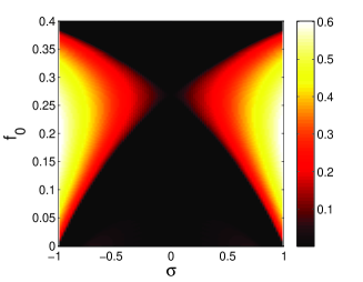
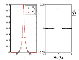
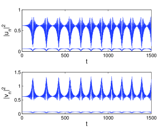
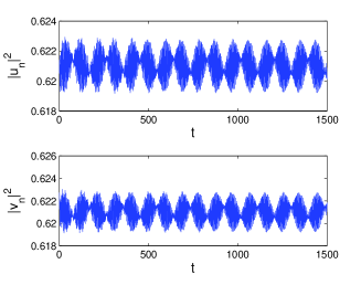
Figure 1: (Color online) The top top left panel shows the (in)stability regions for the onsite discrete solitons in the $(\sigma,f_{0})$ plane with $\kappa_{1}=\kappa_{2}=0.2$. The top right panel depicts a generic example of the soliton’s profile and its stability spectrum at $f_{1}=5.4$. The bottom panels shows the evolution of the two components $|u_{n}|^{2}$ and $|v_{n}|^{2}$, at $n=25,26$ (left) and $n=25$ (right), for $f_{1}=5.4\,$and $5.6$, as found from simulations of the underlying equations (1), which indicates a perfect agreement with the threshold value predicted by the averaged equation.

As seen in the top left panel, for $f_{0}=0.25$, the stability window of the localized mode is $-0.1072<\sigma<0.1084$. Using Eq. (4), we conclude that the values of $f_{1}$ supporting the stable onsite mode are given by $5.5<f_{1}<6.54$ for $\Omega=10$. In the top right panel we present the profile of the discrete soliton at $f_{1}=5.4$ and its stability spectrum. The solution is unstable due to a collision of a pair of eigenvalues at the origin, resulting in a doublet of purely imaginary eigenvalues.

To check the accuracy of the predictions provided by the averaged equations (5), we use the static solution obtained from these equations as initial conditions for simulations of underlying equations (1), inverting transformation (2) for this purpose. Shown in the left bottom panel of Fig. 1 is the generated evolution of the discrete soliton, just near the stability border shown in the top right panel of the same figure. One can see that the unstable soliton tends to rearrange itself into a different time-periodic localized solution. We will see later that in the averaged equation (3) this corresponds to an asymmetric mode. On the other hand, in the right bottom panel we show the evolution of a stable onsite soliton at $f_{1}=5.6$, from which one can conclude that our averaged equations accurately predict the stability threshold, in comparison with Eqs. (1).

III.3 Two-site modes

Proceeding from the fundamental onsite solitons (single-site modes) to the consideration of multi-site ones, a natural object is an in-phase two-site state, i.e., an intersite discrete soliton. However, our numerical analysis (not shown here) reveals that this mode is unstable, in terms of the averaged equations, for all parameter values. Explicit simulations of the evolution of the counterpart of this state within the framework of the original equations (1) confirm its instability.

Next, we consider an out-of-phase fundamental two-site state, alias a twisted localized state, which, in the anticontinuum limit, is seeded by ansatz $U_{n}=V_{n}=\delta_{n,n_{0}}-\delta_{n,n_{0}+1}$. Results of the numerical analysis of this family of odd discrete solitons are presented in Fig. 2. With $\kappa_{1}=\kappa_{2}=0.05$ and $f_{1}=4$, which corresponds to $\sigma=0.455$, the mode is unstable in the range of $0.223<f_{0}<0.469$. In the left and right bottom panels of the figure, we show the evolution of the twisted mode for $f_{0}=0.22$ and $f_{0}=0.23$, respectively. Again we observe a good agreement between the stability threshold predicted by averaged equations (3) and the original system, Eqs. (1).

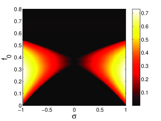
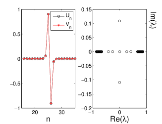
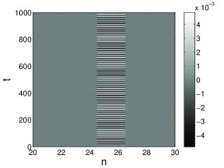
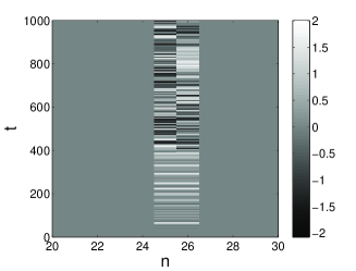
Figure 2: (Color online) The top left panel is the same as in Fig. 1, but for a twisted mode with $\kappa_{1}=\kappa_{2}=0.05$. The top right panel shows the profile of the mode and its stability spectrum for $f_{1}=4$ and $f_{0}=0.23$. Bottom panels show the evolution of stable and an unstable modes at $f_{0}=0.22$ and $\,0.23$, respectively.

IV Symmetry breaking: Pitchfork and Hopf bifurcations

As reported in Refs. TM and herr07 , linearly coupled two-component systems, which are similar to the present one, give rise to a symmetry-breaking bifurcation, which generates asymmetric solitons, while destabilizing symmetric fundamental ones. The analysis of the present model reveals that a similar bifurcation occurs in averaged equations (3), and it generates the respective asymmetric mode. Presented in the top left panel of Fig. 3 is the (in)stability region of the asymmetric mode for $\kappa_{1}=\kappa_{2}=0.2$. In this panel, the white curve designates the bifurcation line, below which the asymmetric mode exists. The analysis demonstrates that the bifurcation in the averaged system (3) is of the pitchfork type, like in the recently studied related models TM ; herr07 ). As a particular example, we depict in the top right panel of Fig. 3 the solution and the stability spectral plane for an unstable asymmetric onsite mode with $f_{0}=0.23$ and $f_{1}=7$, which corresponds to $\sigma=-0.19$.

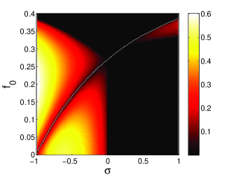
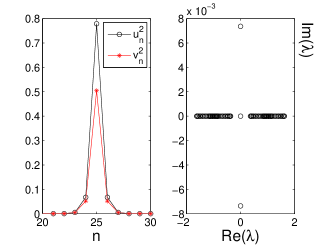
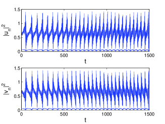
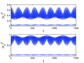
Figure 3: (Color online) The same as in Fig. 1, but for the asymmetric mode, generated by the symmetry-breaking bifurcation, which happens along the while curve in the top left panel. See the text for further details.

It is worthy to note that the stability border of the asymmetric mode in the top left panel exactly corresponds to $\sigma=0$, the asymmetric discrete soliton being stable at $\sigma>0$. This observation may be explained by the fact that the self-phase-modulation nonlinear terms in Eqs. (3) dominate over their cross-phase-modulation counterparts just at $\sigma>0$.

Before we proceed to checking the accuracy of the averaged equations, it is necessary to make the following notice concerning transformation (2): if $|\Phi_{n}(t)|^{2}$ and $|\Psi_{n}(t)|^{2}$ are static, then $|u_{n}(t)|^{2}$ and $|v_{n}(t)|^{2}$ will also be static, provided that $U_{n}$ and $V_{n}$ are symmetric. On the other hand, if $U_{n}$ and $V_{n}$ are asymmetric, the transformation yields $|u_{n}(t)|^{2}$ and $|v_{n}(t)|^{2}$ oscillating periodically in time. Therefore, the pitchfork bifurcation in the averaged equations (5) corresponds to a Hopf bifurcation in the original system (1).

Taking the above-mentioned fact into regard, an unstable asymmetric mode in the averaged equations is expected to correspond to an unstable periodic solution of Eqs. (1). In the bottom left panel of Fig. 3, we display the dynamics of the mode shown in the top right panel of the same figure, represented by $u_{25}$ and $v_{25}$. It is seen that the oscillating solution is indeed unstable, as predicted by the averaged system.

As another test of the accuracy of the approximation based on the averaging method, in the bottom right panel of Fig. 3 we display the dynamics of a stable asymmetric mode with $f_{1}=6$ ($\sigma=4.15\times 10^{-5}$), as produced by direct simulations of the original equations (1). Again, we observe a reasonable agreement between the two systems.

V Conclusion

In this work, we have studied discrete solitons in the system of two linearly coupled DNLSEs (discrete nonlinear Schrödinger equations), which describes several physical situations in BEC. For the case of the coupling constant rapidly varying in time, we have derive the averaged system of coupled generalized DNLSEs. In addition to the linear coupling, the latter system contains nonlinear interaction terms of the four-wave-mixing type. We have constructed families of symmetric single-site localized states (fundamental discrete solitons), as well as in-phase and twisted two-site modes, and identified their stability regions. In particular, the two-site in-phase states are completely unstable, while their twisted counterparts have a stability area. The symmetry-breaking bifurcation of the fundamental discrete soliton, and the resulting asymmetric fundamental localized mode have been found too, and the stability of the asymmetric mode was explored. By means of direct simulations, it was verified that, in all the cases, the averaged equations provide for a very accurate approximation, in comparison with the underlying system featuring the rapidly varying linear coupling.

References

- (1) B. A. Malomed, Soliton Management in Periodic Systems (Springer: New York, 2006).
- (2) L. D. Landau, E. M. Lifshitz, Mechanics (Nauka Publishers: Moscow, 1973).
- (3) M. J. Ablowitz and Z. H. Musslimani, Phys. Rev. Lett. 87, 254102 (2001).
- (4) F. Kh. Abdullaev, E. N. Tsoy, B. A. Malomed, and R. A. Kraenkel, Phys. Rev. A 68, 053606 (2003).
- (5) J. Garnier, F. Kh. Abdullaev, and M. Salerno, Phys. Rev. E 75, 016615 (2007).
- (6) F. A. B. F. de Moura, I. Gleria, I. F. dos Santos, M. L. Lyra, arXiv:0908.1925
- (7) F. Kh. Abdullaev, R. A. Kraenkel, Phys. Rev. A 62, 023613 (2000).
- (8) V. Shchesnovich, B. A. Malomed, and R. A. Kraenkel, Physica D 188, 213 (2004).
- (9) H. Saito, R. G. Hulet, and. M. Ueda, Phys. Rev. A 76, 053619 (2007).
- (10) H. Susanto, P. G. Kevrekidis, B. A. Malomed, and F. Kh. Abdullaev, Phys. Lett. A 372, 1631 (2008).
- (11) M. Zaccanti, C. D’Errico, F. Ferlaino, G. Roati, M. Inguscio, and G. Modugno, Phys. Rev. A 74, 041605(R) (2006), and references therein.
- (12) A. Gubeskys and B. A. Malomed, Phys. Rev. A 75, 063602 (2007).
- (13) G. Herring, P. G. Kevrekidis. B. A. Malomed, R. Carretero-González, and D. J. Frantzeskakis, Phys. Rev. E 76, 066606 (2007).
- (14) W. L. Kath and T. S. Yang, Opt. Lett. 22, 985 (1997).