Energy-Efficient Precoding for
Multiple-Antenna Terminals

Abstract

The problem of energy-efficient precoding is investigated when the terminals in the system are equipped with multiple antennas. Considering static and fast-fading multiple-input multiple-output (MIMO) channels, the energy-efficiency is defined as the transmission rate to power ratio and shown to be maximized at low transmit power. The most interesting case is the one of slow fading MIMO channels. For this type of channels, the optimal precoding scheme is generally not trivial. Furthermore, using all the available transmit power is not always optimal in the sense of energy-efficiency (which, in this case, corresponds to the communication-theoretic definition of the goodput-to-power (GPR) ratio). Finding the optimal precoding matrices is shown to be a new open problem and is solved in several special cases: 1. when there is only one receive antenna; 2. in the low or high signal-to-noise ratio regime; 3. when uniform power allocation and the regime of large numbers of antennas are assumed. A complete numerical analysis is provided to illustrate the derived results and stated conjectures. In particular, the impact of the number of antennas on the energy-efficiency is assessed and shown to be significant.

I Introduction

In many areas, like finance, economics or physics, a common way of assessing the performance of a system is to consider the ratio of what the system delivers to what it consumes. In communication theory, transmit power and transmission rate are respectively two common measures of the cost and benefit of a transmission. Therefore, the ratio transmission rate (say in bit/s) to transmit power (in J/s) appears to be a natural energy-efficiency measure of a communication system. An important question is then: what is the maximum amount of information (in bits) that can be conveyed per Joule consumed? As reported in [1], one of the first papers addressing this issue is [2] where the author determines the capacity per unit cost for various versions of the photon counting channel. As shown in [1], the normalized capacity per unit cost for the well-known additive white Gaussian channel model $Y=X+Z$ is maximized for Gaussian inputs and is given by $\lim_{P\rightarrow 0}\frac{\log_{2}\left(1+\frac{P}{\sigma^{2}}\right)}{P}=\frac{1}{\sigma^{2}\ln 2}$, where $\mathbb{E}|X|^{2}=P$ and $Z\sim\mathbb{C}\mathcal{N}(0,\sigma^{2})$. Here, the main message of communication theory to engineers is that energy-efficiency is maximized by operating at low transmit power and therefore at low transmission rates. However, this answer holds for static and single input single output (SISO) channels and it is legitimate to ask: what is the answer for multiple-input multiple-output (MIMO) channels? In fact, as shown in this paper, the case of slow fading MIMO channels is especially relevant to be considered. Roughly speaking, the main reason for this is that, in contrast to static and fast fading channels, in slow fading channels there are outage events which imply the existence of an optimum tradeoff between the number of successfully transmitted bits or blocks (called goodput in [3] and [4]) and power consumption. Intuitively, this can be explained by saying that increasing transmit power too much may result in a marginal increase in terms of quality or effective transmission rate.

First, let us consider SISO slow fading or quasi-static channels. The most relevant works related to the problem under investigation essentially fall into two classes corresponding to two different approaches. The first approach, which is the one adopted by Verdú in [1] and has already been mentioned, is an information-theoretic approach aiming at evaluating the capacity per unit cost or the minimum energy per bit (see e.g., [5], [6], [7], [8]). In [1], two different cases were investigated depending on whether the input alphabet contains or not a zero cost or free symbol. In this paper, only the case where the input alphabet does not contain a zero-cost symbol will be discussed (i.e., the silence at the transmitter side does not convey information). The second approach, introduced in [9] is more pragmatic than the previous one. In [9] and subsequent works [4], [10], the authors define the energy-efficiency of a SISO communication as $u(p)=\frac{Rf(\eta)}{p}$ where $R$ is the effective transmission data rate in bits, $\eta$ the signal-to-noise-plus-interference ratio (SINR) and $f$ is a benefit function (e.g., the success probability of the transmission) which depends on the chosen coding and modulation schemes. To the authors’ knowledge, in all works using this approach ([9], [4], [10], [11], [12], [13], etc.), the same (pragmatic) choice is made for $f$: $f(x)=(1-e^{-\alpha x})^{N}$, where $\alpha$ is a constant and $N$ the block length in symbols. Interestingly, the two mentioned approaches can be linked by making an appropriate choice for $f$. Indeed, if $f$ is chosen to be the complementary of the outage probability, one obtains a counterpart of the capacity per unit cost for slow fading channels and gives an information-theoretic interpretation to the initial definition of [9]. To our knowledge, the resulting performance metric has not been considered so far in the literature. This specific metric, which we call goodput-to-power ratio (GPR), will be considered in this paper. Moreover, we consider MIMO channels where the transmitter and receiver are informed of the channel distribution information (CDI) and channel state information (CSI) respectively. To conclude the discussion on the relevant literature, we note that some authors addressed the problem of energy-efficiency in MIMO communications but they did not consider the proposed energy-efficiency measure based on the outage probability. In this respect, the most relevant works seem to be [15], [16] and [17]. In [15], the authors adopt a pragmatic approach consisting in choosing a certain coding-modulation scheme in order to reach a given target data rate while minimizing the consumed energy. In [16], the authors study the tradeoff between the minimum energy-per-bit versus spectral efficiency for several MIMO channel models in the wide-band regime assuming a zero cost symbol in the input alphabet and unform power allocation over all the antennas. In [17], the authors consider a similar pragmatic approach to the one in [4], [10] and study a multi-user MIMO channel where the transmitters are constrained to using beamforming power allocation strategies.

This paper is structured as follows. In Sec. II, assumptions on the signal model are provided. In Sec. III, the proposed energy-efficiency measure is defined for static and fast-fading MIMO channels. As the case of slow fading channels is non-trivial, it will be discussed separately in Sec. IV. In Sec. IV, the problem of energy-efficient precoding is discussed for general MIMO slow fading channels and solved for the multiple input single output (MISO) case, whereas in Sec. V asymptotic regimes (in terms of the number of antennas and SNR) are assumed. In Sec. VI, simulations illustrating the derived results and stated conjectures are provided. Sec. VII provides concluding remarks and open issues.

II General System Model

We consider a point-to-point communication with multiple antenna terminals. The signal at the receiver is modeled by:

$$\underline{y}(\tau)=\mathbf{H}(\tau)\underline{x}(\tau)+\underline{z}(\tau),$$ (1)

where $\mathbf{H}$ is the $n_{r}\times n_{t}$ channel transfer matrix and $n_{t}$ (resp. $n_{r}$) the number of transmit (resp. receive) antennas. The entries of $\mathbf{H}$ are i.i.d. zero-mean unit-variance complex Gaussian random variables. The vector $\underline{x}$ is the $n_{t}$-dimensional column vector of transmitted symbols and $\underline{z}$ is an $n_{r}$-dimensional complex white Gaussian noise distributed as $\mathcal{N}(\underline{0},\sigma^{2}\mathbf{I})$. In this paper, the problem of allocating the transmit power between the available transmit antennas is considered. We will denote by $\mathbf{Q}=\mathbb{E}[\underline{x}\underline{x}^{H}]$ the input covariance matrix (called the precoding matrix), which translates the chosen power allocation (PA) policy. The corresponding total power constraint is

$$\mathrm{Tr}(\mathbf{Q})\leq\overline{P}.$$ (2)

At last, the time index $\tau$ will be removed for the sake of clarity. In fact, depending on the rate at which $\mathbf{H}$ varies with $\tau$, three dominant classes of channel models can be distinguished:

1. the class of static channels;

2. the class of fast fading channels;

3. the class of slow fading channels.

The matrix $\mathbf{H}$ is assumed to be perfectly known at the receiver (coherent communication assumption) whereas only the statistics of $\mathbf{H}$ are available at the transmitter. The first two classes of channels are considered in Sec. III and the last one is treated in detail in Sec. IV and V.

III Energy-efficient communications over static and fast fading MIMO channels

III-A Case of static channels

Here the frequency at which the channel matrix varies is strictly zero that is, $\mathbf{H}$ is a constant matrix. In this particular context, both the transmitter and receiver are assumed to know this matrix. We are exactly in the same framework as [18]. Thus, for a given precoding scheme $\mathbf{Q}$, the transmitter can send reliably to the receiver $\log_{2}\left|\mathbf{I}_{n_{r}}+\rho\mathbf{H}\mathbf{Q}\mathbf{H}^{H}\right|$ bits per channel use (bpcu) with $\rho=\frac{1}{\sigma^{2}}$. Then, let us define the energy-efficiency of this communication by:

$$G_{\mathrm{static}}(\mathbf{Q})=\frac{\log_{2}\left|\mathbf{I}_{n_{r}}+\rho\mathbf{H}\mathbf{Q}\mathbf{H}^{H}\right|}{\mathrm{Tr}(\mathbf{Q})}.$$ (3)

The energy-efficiency $G_{\mathrm{static}}(\mathbf{Q})$ corresponds to an achievable rate per unit cost for the MIMO channel as defined in [1]. Assuming that the cost of the transmitted symbol $\underline{x}$, denoted by $b[\underline{x}]$, is the consumed energy $b[\underline{x}]=\|\underline{x}\|^{2}=\mathrm{Tr}(\underline{x}\underline{x}^{H})$, the capacity per unit cost defined in [1] is: $\widetilde{C}_{\mathrm{slow}}\triangleq\displaystyle{\sup_{\underline{x},\mathbb{E}[b[\underline{x}]]\leq\overline{P}}}\frac{I(\underline{x};\underline{y})}{\mathbb{E}[b[\underline{x}]]}$. The supremum is taken over the p.d.f. of $\underline{x}$ such that the average transmit power is limited $\mathbb{E}[b[\underline{x}]]\leq\overline{P}$.

It is easy to check that:

$$\begin{array}[]{lcl}\widetilde{C}_{\mathrm{slow}}&=&\displaystyle{\sup_{\mathbf{Q},\mathrm{Tr}(Q)\leq\overline{P}}}\frac{1}{\mathrm{Tr}(Q)}\ \ \displaystyle{\sup_{\underline{x},\mathbb{E}(\underline{x}\underline{x}^{H})=\mathbf{Q}}}I(\underline{x};\underline{y})\\ &=&\displaystyle{\sup_{\mathbf{Q},\mathrm{Tr}(\mathbf{Q})\leq\overline{P}}}G_{\mathrm{static}}(\mathbf{Q}).\end{array}$$ (4)

The second equality follows from [18] where Telatar proved that the mutual information for the MIMO static channel is maximized using Gaussian random codes. In other words, finding the optimal precoding matrix which maximizes the energy-efficiency function corresponds to finding the capacity per unit cost of the MIMO channel where the cost of a symbol is the necessary power consumed to be transmitted. The question is then whether the strategy “transmit at low power” (and therefore at a low transmission rate) to maximize energy-efficiency, which is optimal for SISO channels, also applies to MIMO channels. The answer is given by the following proposition, which is proved in Appendix A.

Proposition III.1 (Static MIMO channels)

The energy-efficiency of a MIMO communication over a static channel, measured by $G_{\mathrm{static}}$, is maximized when $\mathbf{Q}=\mathbf{0}$ and this maximum is

$$G_{\mathrm{static}}^{*}=\frac{1}{\ln 2}\frac{\mathrm{Tr}(\mathbf{H}\mathbf{H}^{H})}{n_{t}\sigma^{2}}.$$ (5)

Therefore, we see that, for static MIMO channels, the energy-efficiency defined in Eq. (3) is maximized by transmitting at a very low power. This kind of scenario occurs for example, when deploying sensors in the ocean to measure a temperature field (which varies very slowly). In some applications however, the rate obtained by using such a scheme can be not sufficient. In this case, considering the benefit to cost ratio can turn out to be irrelevant, meaning that other performance metrics have to be considered (e.g., minimize the transmit power under a rate constraint).

III-B Case of fast fading channels

In this section, the frequency with which the channel matrix varies is the reciprocal of the symbol duration ($\underline{x}(\tau)$ being a symbol). This means that it can be different for each channel use. Therefore, the channel varies over a transmitted codeword (or packet) and, more precisely, each codeword sees as many channel realizations as the number of symbols per codeword. Because of the corresponding self-averaging effect, the following transmission rate (also called EMI for ergodic mutual information) can be achieved on each transmitted codeword by using the precoding strategy $\mathbf{Q}$ :

$$R_{\mathrm{fast}}(\mathbf{Q})=\mathbb{E}_{\mathbf{H}}\left[\log_{2}\left|\mathbf{I}_{n_{r}}+\rho\mathbf{H}\mathbf{Q}\mathbf{H}^{H}\right|\right].$$ (6)

Interestingly, $R_{\mathrm{fast}}(\mathbf{Q})$ can be maximized w.r.t. $\mathbf{Q}$ by knowing only the statistics of $\mathbf{H}$ that is, $\mathbb{E}\left[\mathbf{H}\mathbf{H}^{H}\right]$, under the standard assumption that the entries of $\mathbf{H}$ are complex Gaussian random variables. In practice, this means that only the knowledge of the path loss, power-delay profile, antenna correlation profile, etc is required at the transmitter to maximize the transmission rate. At the receiver however, the instantaneous knowledge of $\mathbf{H}$ is required. In this framework, let us define energy-efficiency by:

$$G_{\mathrm{fast}}(\mathbf{Q})=\frac{\mathbb{E}_{\mathbf{H}}\left[\log_{2}\left|\mathbf{I}_{n_{r}}+\rho\mathbf{H}\mathbf{Q}\mathbf{H}^{H}\right|\right]}{\mathrm{Tr}(\mathbf{Q})}.$$ (7)

By defining $\underline{g}_{i}$ as the $i$-th column of the matrix $\sqrt{\rho}\mathbf{H}\mathbf{U}$, $i\in\{1,\ldots,n_{t}\}$, $\mathbf{U}$ and $\{p_{i}\}_{i=1}^{n_{t}}$ an eigenvector matrix and the corresponding eigenvalues of $\mathbf{Q}$ respectively, and also by rewriting $G_{\mathrm{fast}}(\mathbf{Q})$ as

$${G_{\mathrm{fast}}(\mathbf{Q})=\mathbb{E}_{\mathbf{H}}\left[\frac{\log_{2}\left|\mathbf{I}_{n_{r}}+\displaystyle{\sum_{i=1}^{n_{t}}p_{i}\underline{g}_{i}\underline{g}_{i}^{H}}\right|}{\displaystyle{\sum_{i=1}^{n_{t}}p_{i}}}\right]},$$ (8)

it is possible to apply the proof of Prop. III.1 for each realization of the channel matrix. This leads to the following result.

Proposition III.2 (Fast fading MIMO channels)

The energy-efficiency of a MIMO communication over a fast fading channel, measured by $G_{\mathrm{fast}}$, is maximized when $\mathbf{Q}=\mathbf{0}$ and this maximum is

$$G_{\mathrm{fast}}^{*}=\frac{1}{\ln 2}\frac{\mathrm{Tr}(\mathbb{E}\left[\mathbf{H}\mathbf{H}^{H}\right])}{n_{t}\sigma^{2}}.$$ (9)

We see that, for fast fading MIMO channels, maximizing energy-efficiency also amounts to transmitting at low power. Interestingly, in slow fading MIMO channels, where outage events are unavoidable, we have found that the answer can be different. This is precisely what is shown in the remaining of this paper.

IV Slow fading MIMO channels: from the general case to special cases

IV-A General MIMO channels

In this section and the remaining of this paper, the frequency with which the channel matrix varies is the reciprocal of the block/codeword/frame/packet/time-slot duration that is, the channel remains constant over a codeword and varies from block to block. As a consequence, when the channel matrix remains constant over a certain block duration much smaller than the channel coherence time, the averaging effect we have mentioned for fast fading MIMO channels does not occur here. Therefore, one has to communicate at rates smaller than the ergodic capacity (maximum of the EMI). The maximum EMI is therefore a rate upper bound for slow fading MIMO channels and only a fraction of it can be achieved (see [27] for more information about the famous diversity-multiplexing tradeoff). In fact, since the mutual information is a random variable, varying from block to block, it is not possible (in general) to guarantee at $100\ \%$ that it is above a certain threshold. A suited performance metric to study slow-fading channels [14] is the probability of an outage for a given transmission rate target $R$. This metric allows one to quantify the probability that the rate target $R$ is not reached by using a good channel coding scheme and is defined as follows:

$$\mathrm{P}_{\mathrm{out}}(\mathbf{Q},R)=\mathrm{Pr}\left[\log_{2}\left|\mathbf{I}_{n_{r}}+\rho\mathbf{H}\mathbf{Q}\mathbf{H}^{H}\right|<R\right].$$ (10)

In terms of information assumptions, here again, it can be checked that only the second-order statistics of $\mathbf{H}$ are required to optimize the precoding matrix $\mathbf{Q}$ (and therefore the power allocation policy over its eigenvalues). In this framework, we propose to define the energy-efficiency as follows:

$$\Gamma(\mathbf{Q},R)=\frac{R[1-\mathrm{P}_{\mathrm{out}}(\mathbf{Q},R)]}{\mathrm{Tr}(\mathbf{Q})}.$$ (11)

In other words, the energy-efficiency or goodput-to-power ratio is defined as the ratio between the expected throughput (see [3],[20] for details) and the average consumed transmit power. The expected throughput can be seen as the average system throughput over many transmissions. In contrast with static and fast fading channels, energy-efficiency is not necessarily maximized at low transmit powers. This is what the following proposition indicates.

Proposition IV.1 (Slow fading MIMO channels)

The goodput-to-power ratio $\Gamma(\mathbf{Q},R)$ is maximized, in general, for $\mathbf{Q}\neq\mathbf{0}$.

The proof of this result is given in Appendix B. Now, a natural issue to be considered is the determination of the matrix (or matrices) maximizing the goodput-to-power ratio (GPR) in slow fading MIMO channels. It turns out that the corresponding optimization problem is not trivial. Indeed, even the outage probability minimization problem w.r.t. $\mathbf{Q}$ (which is a priori simpler) is still an open problem [18], [21], [22]. This is why we only provide here a conjecture on the solution maximizing the GPR.

Conjecture IV.2 (Optimal precoding matrices)

There exists a power threshold $\overline{P}_{0}$ such that:

• if $\overline{P}\leq\overline{P}_{0}$ then $\mathbf{Q}^{*}\in\displaystyle{\arg\min_{\mathbf{Q}}}P_{\mathrm{out}}(\mathbf{Q},R)$ $\ \Rightarrow\$ $\mathbf{Q}^{*}\in\displaystyle{\arg\max_{\mathbf{Q}}}\Gamma(\mathbf{Q},R)$;

• if $\overline{P}>\overline{P}_{0}$ then $\Gamma(\mathbf{Q},R)$ has a unique maximum in $\mathbf{Q}^{*}=\frac{p^{*}}{n_{t}}\mathbf{I}_{n_{t}}$ where $p^{*}\leq\overline{P}$.

This conjecture has been validated for all the special cases solved in this paper. One of the main messages of this conjecture is that, if the available transmit power is less than a threshold, maximizing the GPR is equivalent to minimizing the outage probability. If it is above the threshold, uniform power allocation is optimal and using all the available power is generally suboptimal in terms of energy-efficiency. Concerning the optimization problem associated with (11) several comments are in order. First, there is no loss of optimality by restricting the search for optimal precoding matrices to diagonal matrices: for any eigenvalue decomposition $\mathbf{Q}=\mathbf{U}\mathbf{D}\mathbf{U}^{H}$ with $\mathbf{U}$ unitary and $\mathbf{D}=\mathrm{\textbf{Diag}}(\underline{p})$ with $\underline{p}=(p_{1},\ldots,p_{n_{t}})$, both the outage and trace are invariant w.r.t. the choice of $\mathbf{U}$ and the energy-efficiency can be written as:

$$\Gamma(\mathbf{D},R)=\frac{R[1-\mathrm{P}_{\mathrm{out}}(\mathbf{D},R)]}{\displaystyle{\sum_{i=1}^{n_{t}}}p_{i}}.$$ (12)

Second, the GPR is generally not concave w.r.t. $\mathbf{D}$. In Sec. IV-B, which is dedicated to MISO systems, a counter-example where it is not quasi-concave (and thus not concave) is provided.

Uniform Power Allocation policy

An interesting special case is the one of uniform power allocation (UPA): $\mathbf{D}=\frac{p}{n_{t}}\mathbf{I}_{n_{t}}$ where $p\in[0,\overline{P}]$ and $\Gamma_{\mathrm{UPA}}(p,R)\triangleq\Gamma\left(\frac{p}{n_{t}}\mathbf{I}_{n_{t}},R\right)$.

One of the reasons for studying this case is that the famous conjecture of Telatar given in [18]. This conjecture states that, depending on the channel parameters and target rate (i.e., $\sigma^{2}$, $R$), the power allocation (PA) policy minimizing the outage probability is to spread all the available power uniformly over a subset of $\ell^{*}\in\{1,\ldots,n_{t}\}$ antennas. If this can be proved, then it is straightforward to show that the covariance matrix $\mathbf{D}^{*}$ that maximizes the proposed energy-efficiency function is $\frac{p^{*}}{\ell^{*}}\mathrm{\textbf{Diag}}(\underline{e}_{\ell^{*}})$, where $\underline{e}_{\ell^{*}}\in\mathcal{S}_{\ell^{*}}$. Thus, $\mathbf{D}^{*}$ has the same structure as the covariance matrix minimizing the outage probability except that using all the available power is not necessarily optimal, $p^{*}\in[0,\overline{P}]$. In conclusion, solving Conjecture IV.2 reduces to solving Telatar’s conjecture and also the UPA case.

The main difficulty in studying the outage probability or/and the energy-efficiency function is the fact that the probability distribution function of the mutual information is generally intractable. In the literature, the outage probability is often studied by assuming a UPA policy over all the antennas and also using the Gaussian approximation of the p.d.f. of the mutual information. This approximation is valid in the asymptotic regime of large number of antennas. However, simulations show that it also quite accurate for reasonable small MIMO systems [23], [24].

Under the UPA policy assumption, the GPR $\Gamma_{\mathrm{UPA}}(p,R)$ is conjectured to be quasi-concave w.r.t. $p$. Quasi-concavity is not only useful to study the maximum of the GPR but is also an attractive property in some scenarios such as the distributed multiuser channels. For example, by considering MIMO multiple access channels with single-user decoding at the receiver, the corresponding distributed power allocation game where the transmitters’ utility functions are their GPR is guaranteed to have a pure Nash equilibrium after Debreu-Fan-Glicksberg theorem [25].

Before stating the conjecture describing the behavior of the energy-efficiency function when the UPA policy is assumed, we study the limits when $p\rightarrow 0$ and $p\rightarrow+\infty.$ First, let us prove that $\displaystyle{\lim_{p\rightarrow 0}\Gamma_{\mathrm{UPA}}(p,R)=0}$. Observe that $\displaystyle{\lim_{p\rightarrow 0}P_{\mathrm{out}}\left(\frac{p}{n_{t}}\mathbf{I}_{n_{t}},R\right)=1}$ and thus the limit is not trivial to prove. The result can be proven by considering the equivalent $1+\frac{\rho p}{n_{t}}\mathrm{Tr}(\mathbf{H}\mathbf{H}^{H})$ of the determinant $\left|\mathbf{I}_{n_{r}}+\frac{\rho p}{n_{t}}\mathbf{H}\mathbf{H}^{H}\right|$ when $\sigma\rightarrow+\infty$. As the entries of the matrix $\mathbf{H}$ are i.i.d. complex Gaussian random variables, the quantity $\mathrm{Tr}(\mathbf{H}\mathbf{H}^{H})=\displaystyle{\sum_{i=1}^{n_{t}}\sum_{j=1}^{n_{r}}}|h_{ij}|^{2}$ is a $2n_{r}n_{t}$ Chi-square distributed random variable. Thus $\Gamma_{\mathrm{UPA}}(p,R)$ can be approximated by: $\widehat{\Gamma}_{\mathrm{UPA}}(p,R)=R\exp\left(-\frac{d}{p}\right)\displaystyle{\sum_{k=0}^{n_{r}n_{t}-1}}\frac{d^{k}}{k!}\frac{1}{p^{k+1}}$ with $d=n_{t}(2^{R}-1)\sigma^{2}$. It is easy to see that this approximate tends to zero when $p\rightarrow 0$. Second, note that the limit $\displaystyle{\lim_{p\rightarrow+\infty}\Gamma_{\mathrm{UPA}}(p,R)=0}$. This is easier to check since $\displaystyle{\lim_{p\rightarrow+\infty}P_{\mathrm{out}}\left(\frac{p}{n_{t}}\mathbf{I},R\right)=0}$.

Conjecture IV.3 (UPA and quasi-concavity of the GPR)

Assume that $\mathbf{D}=\frac{p}{n_{t}}\mathbf{I}_{n_{t}}$. Then $\Gamma_{\mathrm{UPA}}(p,R)$ is quasi-concave w.r.t. $p\in\left[0,\overline{P}\right]$.

Table I distinguishes between what has been proven in this paper and the conjectures which remain to be proven.

	Is $\mathbf{D}^{*}$ known?	Is $\Gamma^{\mathrm{UPA}}(p)$ quasi-concave?	Is $p^{*}$ known?
General MIMO	Conjecture	Conjecture	Conjecture
MISO	Yes	Yes	Yes
$1\times 1$	Yes	Yes	Yes
Large MIMO	Conjecture	Yes	Yes
Low SNR	Yes	Yes	Yes
High SNR	Yes	Yes	Conjecture

TABLE I: Summary of proved results and open problems

IV-B MISO channels

In this section, the receiver is assumed to use a single antenna that is, $n_{r}=1$, while the transmitter can have an arbitrary number of antennas, $n_{t}\geq 1$. The channel transfer matrix becomes a row vector $\underline{h}=(h_{1},...,h_{n_{t}})$. Without loss of optimality, the precoding matrix is assumed to be diagonal and is denoted by $\mathbf{D}=\mathrm{\textbf{Diag}}(\underline{p})$ with $\underline{p}^{T}=(p_{1},...,p_{n_{t}})$. Throughout this section, the rate target $R$ and noise level $\sigma^{2}$ are fixed and the auxiliary quantity $c$ is defined by: $c=\sigma^{2}(2^{R}-1)$. By exploiting the existing results on the outage probability minimization problem for MISO channels [22], the following proposition can be proved (Appendix C).

Proposition IV.4 (Optimum precoding matrices for MISO channels)

For all $\ell\in\{1,...,n_{t}-1\}$, let $c_{\ell}$ be the unique solution of the equation (in $x$) $\mathrm{Pr}\left[\frac{1}{\ell+1}\displaystyle{\sum_{i=1}^{\ell+1}}|X_{i}|^{2}\leq x\right]-\mathrm{Pr}\left[\frac{1}{\ell}\displaystyle{\sum_{i=1}^{\ell}}|X_{i}|^{2}\leq x\right]=0$ where $X_{i}$ are i.i.d. zero-mean Gaussian random variables with unit variance. By convention $c_{0}=+\infty$, $c_{n_{t}}=0$. Let $\nu_{n_{t}}$ be the unique solution of the equation (in $y$) $\frac{y^{n_{t}}}{(n_{t}-1)!}-\displaystyle{\sum_{i=0}^{n_{t}-1}}\frac{y^{i}}{i!}=0$. Then the optimum precoding matrices have the following form:

$$\mathbf{D}^{*}=\left|\begin{array}[]{cl}\frac{\overline{P}}{\ell}\mathrm{\textbf{Diag}}(\underline{e}_{\ell})&\ \mathrm{if}\ \overline{P}\in\left[\frac{c}{c_{\ell-1}},\frac{c}{c_{\ell}}\right)\\ \min\left\{\frac{\sigma^{2}(2^{R}-1)}{\nu_{n_{t}}},\frac{\overline{P}}{n_{t}}\right\}\mathbf{I}&\ \mathrm{if}\ \overline{P}\geq\frac{c}{c_{n_{t}-1}}\end{array}\right.$$ (13)

where $c=\sigma^{2}(2^{R}-1)$ and $\underline{e}_{\ell}\in\mathcal{S}_{\ell}$.

Similarly to the optimal precoding scheme for the outage probability minimization, the solution maximizing the GPR consists in allocating the available transmit power uniformly between only a subset $\ell\leq n_{t}$ antennas. As i.i.d entries are assumed for $\mathbf{H}$, the choice of these antennas does not matter. What matters is the number of antennas selected (denoted by $\ell$), which depends on the available transmit power $\overline{P}$: the higher the transmit power, the higher the number of used antennas. The difference between the outage probability minimization and GPR maximization problems appears when the transmit power is greater than the threshold $\frac{c}{c_{n_{t}-1}}$. In this regime, saturating the power constraint is suboptimal for the GPR optimization. The corresponding sub-optimality becomes more and more severe as the noise level is low; simulations (Sec. VI) will help us to quantify this gap.

Unless otherwise specified, we will assume from now on that UPA is used at the transmitter. This assumption is, in particular, useful to study the regime where the available transmit power is sufficiently high (as conjectured in Proposition IV.1). Under this assumption, our goal is to prove that the GPR is quasi-concave w.r.t. $p\in[0,\overline{P}]$ with $\mathbf{D}=\frac{p}{n_{t}}\mathbf{I}_{n_{t}}$ and determine the (unique) solution $p^{*}$ which maximizes the GPR. Note that the quasi-concavity property w.r.t. $\underline{p}$ is not always available for MISO systems (and thus is not always available for general MIMO channels). In Appendix D, a counter-example proving that in the case where $n_{r}=1$ and $n_{t}=2$ (two input single output channel, TISO) the energy-efficiency $\Gamma^{\mathrm{TISO}}\left(\textbf{Diag}(\underline{p}),R\right)$ is not quasi-concave w.r.t. $\underline{p}=(p_{1},p_{2})$ is provided.

Proposition IV.5 (UPA and quasi-concavity (MISO channels))

Assume the UPA, $\mathbf{Q}=\frac{p}{n_{t}}\mathbf{I}_{n_{t}}$, then $\Gamma(p,R)$ is quasi-concave w.r.t. $p\in\left[0,\overline{P}\right]$ and has a unique maximum point in $p^{*}=\min\left\{\frac{(2^{R}-1)n_{t}\sigma^{2}}{\nu_{n_{t}}},\overline{P}\right\}$ where $\nu_{n_{t}}$ is the solution (w.r.t. $y$) of:

$$\frac{y^{n_{t}}}{(n_{t}-1)!}-\displaystyle{\sum_{i=0}^{n_{t}-1}}\frac{y^{i}}{i!}=0.$$ (14)

Proof:

Since the entries of $\underline{h}$ are complex Gaussian random variables, the sum $\displaystyle{\sum_{k=1}^{n_{t}}}|h_{k}|^{2}$ is a $2n_{t}-$ Chi-square distributed random variable, which implies that:

$$\begin{array}[]{lcl}\Gamma^{\mathrm{MISO}}(p,R)&=&\displaystyle{\frac{R\left\{1-\mathrm{Pr}[\log_{2}\left(1+\frac{\rho p}{n_{t}}\underline{h}^{H}\underline{h}\right)<R]\right\}}{p}}\\ &=&\displaystyle{\frac{R\left\{1-\mathrm{Pr}\left[\displaystyle{\sum_{i=1}^{n_{t}}}|h_{i}|^{2}<\frac{d}{p}\right]\right\}}{p}}\\ &=&\displaystyle{R\times\mathrm{e}^{-\frac{d}{p}}\sum_{i=0}^{n_{t}-1}\frac{d^{i}}{p^{i+1}}\frac{1}{i!}},\end{array}$$ (15)

with $d=cn_{t}=(2^{R}-1)n_{t}\sigma^{2}$. The second order derivative of the goodput $R\left[\mathrm{e}^{-\frac{d}{p}}\displaystyle{\sum_{i=0}^{n_{t}-1}}\left(\frac{d}{p}\right)^{i}\frac{1}{i!}\right]$ w.r.t. $p$ is
$R\left[\frac{d^{n_{t}}}{p^{n_{t}+3}}\frac{1}{n_{t}!}\mathrm{e}^{-d/p}(d-(n_{t}+1)p)\right]$. Clearly, the goodput is a sigmoidal function and has a unique inflection point in $p_{0}=\frac{d}{n_{t}+1}$. Therefore, the function $\Gamma^{\mathrm{MISO}}(p,R)$ is quasi-concave [26] and has a unique maximum in $p^{*}=\min\left\{\frac{d}{\nu_{n_{t}}},\overline{P}\right\}$ where $\nu_{n_{t}}$ is the root of the first order derivative of $\Gamma^{\mathrm{MISO}}(p,R)$ that is, the solution of (14). ∎

The SIMO case ($n_{t}=1$, $n_{r}\geq 2$) follows directly since $|\mathbf{I}+\rho p\underline{h}\underline{h}^{H}|=1+\rho p\underline{h}^{H}\underline{h}$.

To conclude this section, we consider the most simple case of MISO channels namely the SISO case ($n_{t}=1$, $n_{r}=1$). We have readily that:

$$\Gamma^{\mathrm{SISO}}(p,R)=\frac{e^{-\frac{c}{p}}}{p}.$$ (16)

To the authors’ knowledge, in all the works using the energy-efficiency definition of [4] for SISO channels, the only choice of energy-efficiency function made is based on the empirical approximation of the block error rate which is $\frac{(1-e^{-x})^{M}}{x}$, $M$ being the block length and $x$ the operating SINR. Interestingly, the function given by (16) exhibits another possible choice. It can be checked that the function $e^{-\frac{c}{p}}$ is sigmoidal and therefore $\Gamma^{\mathrm{SISO}}$ is quasi-concave w.r.t. $p$ [26]. The first order derivative of $\Gamma^{\mathrm{SISO}}$ is

$$\frac{\partial\Gamma^{\mathrm{SISO}}}{\partial p}=R\frac{(c-p)e^{-\frac{c}{p}}}{p^{3}}.$$ (17)

The GPR is therefore maximized in a unique point which $p^{*}=c=\sigma^{2}(2^{R}-1)$. To make the bridge between this solution and the one derived in [4] for the power control problem over multiple access channels, the optimal power level can be rewritten as:

$$p^{*}=\min\left\{\frac{\sigma^{2}}{\mathbb{E}|h|^{2}}(2^{R}-1),\overline{P}\right\}$$ (18)

where $\mathbb{E}|h|^{2}=1$ in our case. In [4], instantaneous CSI knowledge at the transmitters is assumed while here only the statistics are assumed to be known at the transmitter. Therefore, the power control interpretation of (18) in a wireless scenario is that the power is adapted to the path loss (slow power control) and not to fast fading (fast power control).

V Slow fading MIMO channels in asymptotic regimes

In this section, we first consider the GPR for the case where the size of the MIMO system is finite assuming the low/high SNR operating regime. Then, we consider the UPA policy and prove that Conjecture IV.3 claiming that $\Gamma_{\mathrm{UPA}}(p,R)$ is quasi-concave w.r.t. $p$ (which has been proven for MISO, SIMO, and SISO channels) is also valid in the asymptotic regimes where either at least one dimension of the system ($n_{t}$, $n_{r}$) is large but the SNR is finite. Here again, the theory of large random matrices is successfully applied since it allows one to prove some results which are not available yet in the finite case (see e.g., [19], [28] for other successful examples).

V-A Extreme SNR regimes

Here, all the channel parameters ($n_{t}$, $n_{r}$, and $\overline{P}$ in particular) are fixed. The low (resp. high) SNR regime is defined by $\sigma^{2}\rightarrow+\infty$ (resp. $\sigma^{2}\rightarrow 0$). In both cases, we will consider the GPR and the optimal power allocation problem.

V-A1 Low SNR regime

Let us consider the general power allocation problem where $\mathbf{D}=\mathrm{\textbf{Diag}}(\underline{p})$ with $\underline{p}=(p_{1},\ldots,p_{n_{t}})$. In [22], the authors extended the results obtained in the low and high SNR regimes for the MISO channel to the MIMO case. In the low SNR regime, the authors of [22] proved that the outage probability $P_{\mathrm{out}}(\mathrm{\textbf{Diag}}(\underline{p}),R)$ is a Schur-concave (see [29] for details) function w.r.t. $\underline{p}$. This implies directly that beamforming power allocation policy maximizes the outage probability. These results can be used (see Appendix E) to prove the following proposition:

Proposition V.1 (Low SNR regime)

When $\sigma^{2}\rightarrow+\infty$, the energy-efficiency function $\Gamma(\mathrm{\textbf{Diag}}(\underline{p}),R)$ is Schur-concave w.r.t. $\underline{p}$ and maximized by a beamforming power allocation policy $\mathbf{D}^{*}=\overline{P}\mathrm{\textbf{Diag}}(\underline{e}_{1})$.

V-A2 High SNR regime

Now, let us consider the high SNR regime. It turns out that the UPA policy maximizes the energy-efficiency function. In this case also, the proof of the following proposition is based on the results in [22] (see Appendix E).

Proposition V.2 (High SNR regime)

When $\sigma^{2}\rightarrow 0$, the energy-efficiency function $\Gamma(\mathrm{\textbf{Diag}}(\underline{p}),R)$ is Schur-convex w.r.t. $\underline{p}$ and maximized by an uniform power allocation policy $\mathbf{D}^{*}=\frac{p^{*}}{n_{t}}\mathbf{I}_{n_{t}}$ with $p^{*}\in(0,\overline{P}]$. Furthermore, the limit when $p\rightarrow 0$ such that $\frac{p}{\sigma^{2}}\rightarrow\xi$ is $\Gamma\left(\frac{p}{n_{t}}\mathbf{I}_{n_{t}},R\right)\rightarrow+\infty$ which implies that $p^{*}\rightarrow 0$.

In other words, in the high SNR regime, the optimal structure of the covariance matrix is obtained by uniformly spreading the power over all the antennas, $\mathbf{D}^{*}=\frac{p^{*}}{n_{t}}\mathbf{I}_{n_{t}}$ the same structure which minimizes the outage probability in this case. Nevertheless, in contrast to the outage probability optimization problem, in order to be energy-efficient it is not optimal to use all the available power $\overline{P}$ but to transmit with zero power.

V-B Large MIMO channels

The results we have obtained can be summarized in the following proposition.

Proposition V.3 (Quasi-concavity for large MIMO systems)

If the system operates in one of the following asymptotic regimes:

(a) $n_{t}<+\infty$ and $n_{r}\rightarrow+\infty$;

(b) $n_{t}\rightarrow+\infty$ and $n_{r}<+\infty$;

(c) $n_{t}\rightarrow+\infty$, $n_{r}\rightarrow+\infty$ with $\displaystyle{\lim_{n_{i}\rightarrow+\infty,i\in\{t,r\}}\frac{n_{r}}{n_{t}}=\beta<+\infty}$,

then $\Gamma_{\mathrm{UPA}}(p,R)$ is quasi-concave w.r.t. $p\in[0,\overline{P}]$.

Proof:

Here we prove each of the three statements made above and provide comments on each of them at the same time.

Regime (a): $n_{t}<+\infty$ and $n_{r}\rightarrow\infty$. The idea of the proof is to consider a large system equivalent of the function $\Gamma_{\mathrm{UPA}}(p,R)$. This equivalent is denoted by $\widehat{\Gamma}^{\mathrm{a}}_{\mathrm{UPA}}(p,R)$ and is based on the Gaussian approximation of the mutual information $\log_{2}\left|\mathbf{I}+\frac{\rho p}{n_{t}}\mathbf{H}\mathbf{H}^{H}\right|$ (see e.g., [30]). The goal is to prove that the numerator of $\widehat{\Gamma}^{\mathrm{a}}_{\mathrm{UPA}}(p,R)$ is a sigmoidal function w.r.t. $p$ which implies that $\widehat{\Gamma}^{\mathrm{a}}_{\mathrm{UPA}}(p,R)$ is a quasi-concave function [26]. In the considered asymptotic regime, we know from [30] that:

$$\log_{2}\left|\mathbf{I}+\frac{\rho p}{n_{t}}\mathbf{H}\mathbf{H}^{H}\right|\rightarrow\mathcal{N}\left(n_{t}\log_{2}\left(1+\frac{n_{r}}{n_{t}}\rho p\right),\frac{n_{t}}{n_{r}}\log_{2}(e)\right).$$ (19)

A large system equivalent of the numerator of $\Gamma_{\mathrm{UPA}}(p,R)$, which is denoted by $\widehat{N}_{a}(p,R)$, follows:

$$\widehat{N}_{a}(p,R)=RQ\left(\frac{R-n_{t}\log_{2}\left(1+\frac{n_{r}}{n_{t}}\rho p\right)}{\sqrt{\frac{n_{t}}{n_{r}}\log_{2}(e)}}\right)$$ (20)

where $Q(x)=\frac{1}{\sqrt{2\pi}}\int_{x}^{+\infty}\exp\left(-\frac{t^{2}}{2}\right)\mathrm{d}t$. Denote the argument of $Q$ in (20) by $\alpha_{a}$. The second order derivative of $\widehat{N}_{a}(p,R)$ w.r.t. $p$

$$\frac{\partial^{2}\widehat{N}_{a}(p,R)}{\partial p^{2}}=\frac{1}{\sqrt{2\pi}}\left[\alpha_{a}(p)(\alpha_{a}^{\prime}(p))^{2}-\alpha_{a}^{\prime\prime}(p)\right]\exp\left(-\frac{\alpha_{a}(p)^{2}}{2}\right).$$ (21)

Therefore $\widehat{N}_{a}(p,R)$ has a unique inflection point

$$\tilde{p}_{a}=\frac{n_{t}}{n_{r}\rho}\left\{2^{\left[\frac{1}{n_{t}}\left(R-\frac{1}{n_{t}}\left(\frac{n_{t}\log_{2}(e)}{n_{r}}\right)^{3/2}\right)\right]}-1\right\}.$$ (22)

Clearly, for each equivalent of $\Gamma_{\mathrm{UPA}}(p,R)$, the numerator has a unique inflection point and is sigmoidal, which concludes the proof. In fact, in the considered asymptotic regime we have a stronger result since $\displaystyle{\lim_{n_{r}\rightarrow+\infty}}\tilde{p}_{a}=0$, which implies that $\widehat{N}_{a}(p,R)$ is concave and therefore $\widehat{\Gamma}^{\mathrm{a}}_{\mathrm{UPA}}(p,R)$ is maximized in $p_{a}^{*}=0$ as in the case of static MIMO channels. This translates the well-known channel hardening effect [30]. However, in contrast to the static case, the energy-efficiency becomes infinite here since $\Gamma_{\mathrm{UPA}}(p,R)\rightarrow\frac{1}{p}$ with $p_{a}^{*}\rightarrow 0$.

Regime (b): $n_{t}\rightarrow+\infty$ and $n_{r}<+\infty$. To prove the corresponding result the same reasoning as in (a) is applied. From [30] we know that:

$$\log_{2}\left|\mathbf{I}+\frac{\rho p}{n_{t}}\mathbf{H}\mathbf{H}^{H}\right|\rightarrow\mathcal{N}\left(n_{r}\log_{2}(1+\rho p),\left(\sqrt{\frac{n_{r}}{n_{t}}}\log_{2}(e)\frac{\rho p}{1+\rho p}\right)^{2}\right).$$ (23)

A large system equivalent of the numerator of $\Gamma_{\mathrm{UPA}}(p,R)$ is $\widehat{N}_{b}(p,R)=RQ\left(\alpha_{b}(p)\right)$ with

$$\alpha_{b}(p)=\sqrt{\frac{n_{t}}{n_{r}}}\log_{2}(e)\frac{1+\rho p}{\rho p}[R-n_{r}\log_{2}(1+\rho p)].$$ (24)

The numerator function $\widehat{N}_{b}(p,R)$ can be checked to have a unique inflection point given by:

$$\tilde{p}_{b}=\sigma^{2}\left(2^{\frac{R}{n_{r}}}-1\right)$$ (25)

and is sigmoidal, which concludes the proof. We see that the inflection point does not vanish this time (with $n_{t}$ here) and therefore the function $\widehat{N}_{b}(p,R)$ is quasi-concave but not concave in general. From [26], we know that the optimal solution $p^{*}_{b}$ represents the point where the tangent that passes through the origin intersects the S-shaped function $RQ\left(\alpha_{b}(p)\right)$. As $n_{t}$ grows large, the function $Q\left(\alpha_{b}(p)\right)$ becomes a Heavyside step function since $\forall p\leq\tilde{p}_{b}$, $\lim_{n_{t}\rightarrow+\infty}Q\left(\alpha_{b}(p)\right)=0$ and $\forall p\geq\tilde{p}_{b}$, $\lim_{n_{t}\rightarrow+\infty}Q\left(\alpha_{b}(p)\right)=1$. This means that the optimal power $p^{*}_{b}$ that maximizes the energy-efficiency approaches $\tilde{p}_{b}$ as $n_{t}$ grows large, $p^{*}\scriptsize\footnotesize\small_{b}\rightarrow\sigma^{2}\left(2^{\frac{R}{n_{r}}}-1\right)$. The optimal energy-efficiency tends to $\frac{\widehat{N}_{b}(p^{*}_{b},R)}{p^{*}_{b}}\rightarrow\frac{1}{2\sigma^{2}\left(2^{\frac{R}{n_{r}}}-1\right)}$ when $n_{t}\rightarrow+\infty$.

Regime (c): $n_{t}\rightarrow+\infty$, $n_{r}\rightarrow\infty$. Here we always apply the same reasoning but exploit the results derived in [31]. From [31], we have that:

$$\log_{2}\left|\mathbf{I}+\frac{\rho p}{n_{t}}\mathbf{H}\mathbf{H}^{H}\right|\rightarrow\mathcal{N}\left(n_{t}\mu_{I},\sigma_{I}^{2}\right)$$ (26)

where $\mu_{I}=\beta\log_{2}(1+\rho p(1-\gamma))-\gamma+\log_{2}(1+\rho p(\beta-\gamma))$, $\sigma_{I}^{2}=-\log_{2}\left(1-\frac{\gamma^{2}}{\beta}\right)$,
$\gamma=\frac{1}{2}\left(1+\beta+\frac{1}{\rho p}-\sqrt{(1+\beta+\frac{1}{\rho p})^{2}-4\beta}\right)$. It can be checked that $(\alpha_{c}^{\prime}(p))^{2}\alpha_{c}(p)-\alpha_{c}^{\prime\prime}(p)=0$ has a unique solution where $\alpha_{c}(p)=\frac{R-n_{t}\mu_{I}(p)}{\sigma_{I}(p)}$. We obtain $\alpha_{c}^{\prime}(p)=\frac{n_{t}\mu_{I}\sigma_{I}^{\prime}-n_{t}\mu_{I}^{\prime}\sigma_{I}-R\sigma_{I}^{\prime}}{\sigma_{I}^{2}}$ and
$\alpha_{c}^{\prime\prime}(p)=\frac{(n_{t}\mu_{I}\sigma_{I}^{\prime\prime}-n_{t}\mu_{I}^{\prime\prime}\sigma_{I}-R\sigma_{I}^{\prime\prime})\sigma_{I}^{2}-2\sigma_{I}\sigma_{I}^{\prime}(n_{t}\mu_{I}\sigma_{I}^{\prime}-n_{t}\mu_{I}^{\prime}\sigma_{I}-R\sigma_{I}^{\prime})}{\sigma_{I}^{4}}$. We observe that, in the equation $(\alpha_{c}^{\prime}(p))^{2}\alpha_{c}(p)-\alpha_{c}^{\prime\prime}(p)=0$, there are terms in $n_{t}^{3}$, $n_{t}^{2}$, $n_{t}$ and constant terms w.r.t. $n_{t}$. When $n_{t}$ becomes sufficiently large the first order terms can be neglected, which implies that the solution is given by $\mu_{I}(p)=0$. It can be shown that $\mu_{I}(0)=0$ and that $\mu_{I}$ is an increasing function w.r.t. $p$ which implies that the unique solution is $\tilde{p}_{c}=0$. Similarly to regime (a) we obtain the trivial solution $p_{c}^{*}=0$.

∎

VI Numerical results

In this section, we present several simulations that illustrate our analytical results and verify the two conjectures stated. Since closed-form expressions of the outage probability are not available in general, Monte Carlo simulations will be implemented. The exception is the MISO channel for which the optimal energy-efficiency can be computed numerically (as we have seen in Sec. IV-B) without the need of Monte Carlo simulations.

UPA, the quasi-concavity property and the large MIMO channels.

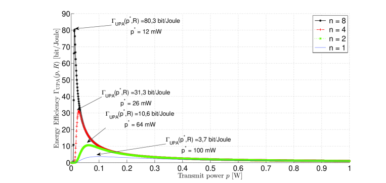
Figure 1: Energy-efficiency (GPR) vs. transmit power $p\in[0,1]$ W for MIMO channels where $n_{r}=n_{t}=n\in\{1,2,4,8\}$, UPA $\mathbf{D}=\frac{p}{n_{t}}\mathbf{I}_{n_{t}}$, $\rho=10$ dB, $R=1$ bpcu. Observe that the energy-efficiency is a quasi-concave function w.r.t. $p$. The optimal point $p^{*}$ is decreasing and $\Gamma_{\mathrm{UPA}}\left(p^{*},R\right)$ is increasing with $n$.

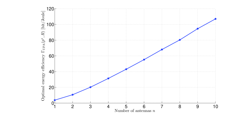
Figure 2: Energy-efficiency vs. the number of antennas $n$ for MIMO $n_{r}=n_{t}=n\in\{1,2,4,8\}$, UPA, $\mathbf{D}=\frac{p}{n_{t}}\mathbf{I}_{n_{t}}$, $\rho=10$ dB, $R=1$ bpcu and $\overline{P}=1$ W. Observe that $\Gamma_{\mathrm{UPA}}\left(p^{*},R\right)$ is increasing with $n$.

Let us consider the case of UPA. In Fig. 1, we plot the GPR $\Gamma_{\mathrm{UPA}}\left(p,R\right)$ as a function of the transmit power $p\in[0,\overline{P}]$ W for an MIMO channel where $n_{r}=n_{t}=n$ with $n\in\{1,2,4,8\}$ and $\rho=10$ dB, $R=1$ bpcu, $\overline{P}=1$ W. First, note that the energy-efficiency for UPA is a quasi-concave function w.r.t. $p$, illustrating Conjecture IV.3. Second, we observe that the optimal power $p^{*}$ maximizing the energy-efficiency function is decreasing and approaching zero as the number of antennas increases and also that $\Gamma_{\mathrm{UPA}}\left(p^{*},R\right)$ is increasing with $n$. In Fig. 2, this dependence of the optimal energy-efficiency and the number of antennas $n$ is depicted explicitly for the same scenario. These observations are in accordance with the asymptotic analysis in subsection V-B for Regime (c).

Similar simulation results were obtained for the case where $n_{t}$ is fixed and $n_{r}$ is increasing, thus illustrating the asymptotic analysis in subsection V-B for Regime (a).

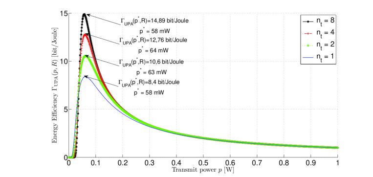
Figure 3: Energy-efficiency vs. transmit power $p\in[0,1]$ W for MIMO $n_{r}=2$, $n_{t}\in\{1,2,4,8\}$, UPA $\mathbf{D}=\frac{p}{n_{t}}\mathbf{I}_{n_{t}}$, $\rho=10$ dB, $R=1$ bpcu. Observe that the energy-efficiency is a quasi-concave function w.r.t. $p$. The optimal point $p^{*}$ is not decreasing with $n$ but almost constant.

In Fig. 3, we plot the energy-efficiency $\Gamma_{\mathrm{UPA}}\left(p,R\right)$ as a function of the transmit power $p\in[0,\overline{P}]$ W for MIMO channel such that $n_{r}=2$, $n_{t}\in\{1,2,4,8\}$ and $\rho=10$ dB, $R=1$ bpcu, $\overline{P}=1$ W. The difference w.r.t. the previous case, is that the optimal power $p^{*}$ does not go to zero when $n_{t}$ increases. This figure illustrates the results obtained for Regime (b) in section V-B where the optimal power allocation $p^{*}_{b}\rightarrow\frac{2^{\frac{R}{n_{r}}}-1}{\rho}=0.0414$ W and the optimal energy-efficiency $\Gamma^{*}_{UPA}\rightarrow\frac{\rho}{2(2^{\frac{R}{n_{r}}}-1)}=12,07$ bit/Joule when $n_{t}\rightarrow+\infty$.

UPA and the finite MISO channel

In Fig. 4, we illustrate Proposition IV.4 for $n_{t}=4$. We trace the cases where the transmitter uses an optimal UPA over only a subset of $\ell\in\{1,2,3,4\}$ antennas for $\rho=10$ dB, $R=3$ bpcu. We observe that: i) if $\overline{P}\leq\frac{c}{c_{1}}$ then the beamforming PA is the generally optimal structure with $\mathrm{D}^{*}=\overline{P}\ \mathrm{\textbf{Diag}}(\underline{e}_{1})$; ii) if $\overline{P}\in\left[\frac{c}{c_{1}}\frac{c}{c_{2}}\right)$ then using UPA over three antennas is the generally optimal structure with $\mathrm{D}^{*}=\overline{P}/2\ \mathrm{\textbf{Diag}}(\underline{e}_{2})$; iii) if $\overline{P}\in\left[\frac{c}{c_{2}}\frac{c}{c_{3}}\right)$ then using UPA over three antennas is generally optimal with $\mathrm{D}^{*}=\overline{P}/3\ \mathrm{\textbf{Diag}}(\underline{e}_{3})$; iv) if $\overline{P}\geq\frac{c}{c_{4}}$ then the UPA over all the antennas is optimal with $\mathrm{D}^{*}=\frac{1}{4}\min\left\{\frac{4*c}{\nu_{4}},\overline{P}\right\}\ \mathbf{I}_{4}$. The saturated regime illustrates the fact that it is not always optimal to use all the available power after a certain threshold.

UPA and the finite MIMO channel

Fig. 5 represents the success probability, $1-P_{\mathrm{out}}(\mathbf{D},R)$, in function of the power constraint $\overline{P}$ for $n_{t}=n_{r}=2$, $R=1$ bpcu, $\rho=3$ dB. Since the optimal PA that maximizes the success probability is unknown (unlike the MISO case) we use Monte-Carlo simulations and exhaustive search to compare the optimal PA with the UPA and the beamforming PA. We observe that the result is in accordance with Telatar’s conjecture. There exists a threshold $\delta=0.16$ W such that if $\overline{P}\leq\delta$, the beamforming PA is optimal and otherwise the UPA is optimal. Of course, using all the available power is always optimal when maximizing the success probability. The objective is to check whether Conjecture IV.2 is verified in this particular case. To this purpose, Fig. 6 represents the energy-efficiency function for the same scenario. We observe that for the exact threshold $\delta=0.16$ W, we obtain that if $\overline{P}\leq\delta$ the beamforming PA using all the available power is optimal. If $\overline{P}>\delta$ the UPA is optimal. Here, similarly to the MISO case, we observe a saturated regime which means that after a certain point it is not optimal w.r.t. energy-efficiency to use up all the available transmit power. In conclusion, our conjecture has been verified in this simulation.

Note that for the beamforming PA case we have explicit relations for both the outage probability and the energy-efficiency (it is easy to check that the MIMO with beamforming PA reduces to the SIMO case) and thus Monte-Carlo simulations have not been used.

VII Conclusion

In this paper, we propose a definition of energy-efficiency metric which is the extension of the work in [1] to static MIMO channels. Furthermore, our definition bridges the gap between the notion of capacity per unit cost [1] and the empirical approach of [4] in the case of slow fading channels. In static and fast fading channels, the energy-efficiency is maximized at low transmit power and the corresponding rates are also small. On the the other hand, the case of slow fading channel is not trivial and exhibits several open problems. It is conjectured that solving the (still open) problem of outage minimization is sufficient to solve the problem of determining energy-efficient precoding schemes. This conjecture is validated by several special cases such as the MISO case and asymptotic cases. Many open problems are introduced by the proposed performance metric, here we just mention some of them:

• First of all, the conjecture of the optimal precoding schemes for general MIMO channels needs to be proven.

• The quasi-concavity of the goodput-to-power ratio when uniform power allocation is assumed remains to be proven in the finite setting.

• A more general channel model should be considered. We have considered i.i.d. channel matrices but considering non zero-mean matrices with arbitrary correlation profiles appears to be a challenging problem for the goodput-to-power ratio.

• The connection between the proposed metric and the diversity-multiplexing tradeoff at high SNR has not been explored.

• Only single-user channels have been considered. Clearly, multi-user MIMO channels such as multiple access or interference channels should be considered.

• The case of distributed multi-user channels become more and more important for applications (unlicensed bands, decentralized cellular networks, etc.). Only one result is mentioned in this paper: the existence of a pure Nash equilibrium in distributed MIMO multiple access channels assuming uniform power allocation transmit policy.

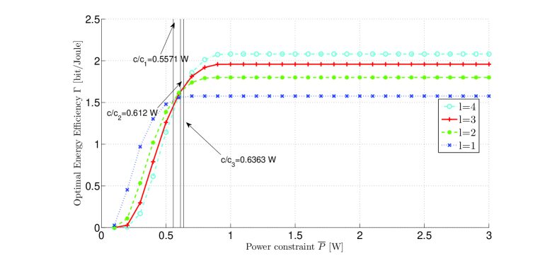
Figure 4: Optimal energy-efficiency vs. constraint power for MISO $n_{t}=4$, $n_{r}=1$, UPA over a subset of $\ell\in\{1,2,3,4\}$ antennas, $\rho=10$ dB, $R=3$ bpcu. We illustrate the results of Proposition IV.4. If $\overline{P}\leq\frac{c}{c_{1}}$ is low enough, the beamforming PA with full power is optimal. If $\overline{P}\geq\frac{c}{c_{2}}$ is high enough, the UPA is optimal but not with full power necessarily $\left(p^{*}=\min\{\frac{c}{\nu_{4}},\overline{P}\}\right)$ which explains the saturated regime.

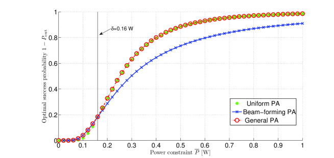
Figure 5: Success probability vs. power constraint $\overline{P}$, comparison between beamforming PA, UPA and General PA for MIMO $n_{t}=n_{r}=2$, $R=1$ bpcu, $\rho=3$ dB. We observe that Telatar’s conjecture is validated. There is a threshold, $\delta=0.16$ W, below which ($\overline{P}\leq\delta$) the beamforming PA is optimal and above it, UPA is optimal.

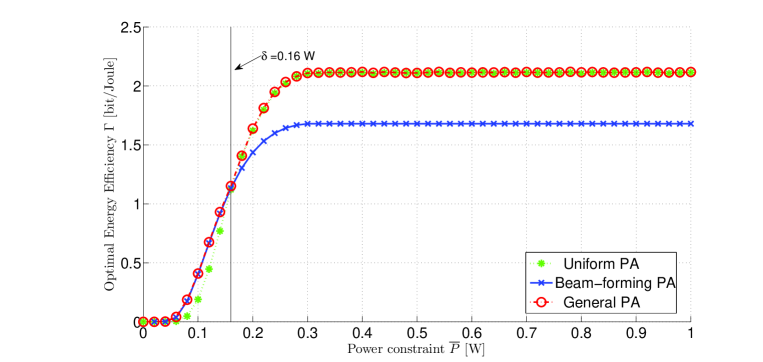
Figure 6: Optimal energy-efficiency vs. power constraint $\overline{P}$, comparison between beamforming PA, UPA and General PA for MIMO $n_{t}=n_{r}=2$, $R=1$ bpcu, $\rho=3$ dB. We observe that our Conjecture IV.2 is validated. For the exact same $\delta=0.16$ W, we have that for $\overline{P}\leq\delta$ the beamforming PA structure optimal and above it, UPA structure is optimal.

Appendix A Proof of Proposition III.1

As $\mathbf{Q}$ is a positive semi-definite Hermitian matrix, it can always be spectrally decomposed as $\mathbf{Q}=\mathbf{U}\mathbf{D}\mathbf{U}^{H}$ where $\mathbf{D}=\mathrm{\textbf{Diag}}(p_{1},\ldots,p_{n_{t}})$ is a diagonal matrix representing a given PA policy and $\mathbf{U}$ a unitary matrix. Our goal is to prove that, for every $\mathbf{U}$, $G_{\mathrm{static}}$ is maximized when $\mathbf{D}=\mathrm{\textbf{Diag}}(0,0,...,0)$. To this end we rewrite $G_{\mathrm{static}}$ as

$${G_{\mathrm{static}}(\mathbf{U}\ \mathrm{\textbf{Diag}}(p_{1},\ldots,p_{n_{t}})\ \mathbf{U}^{H})=\frac{\log_{2}\left|\mathbf{I}_{n_{r}}+\displaystyle{\sum_{i=1}^{n_{t}}p_{i}\underline{g}_{i}\underline{g}_{i}^{H}}\right|}{\displaystyle{\sum_{i=1}^{n_{t}}p_{i}}}},$$ (27)

where $\underline{g}_{i}$ represents the $i^{th}$ column of the $n_{r}\times n_{t}$ matrix $\mathbf{G}=\sqrt{\rho}\mathbf{H}\mathbf{U}$ and proceed by induction on $n_{t}\geq 1$.

First, we introduce an auxiliary quantity (whose role will be made clear a little further)

$$\begin{array}[]{lcl}E^{(n_{t})}(p_{1},\ldots,p_{n_{t}})&\triangleq&\displaystyle{\mathrm{Tr}\left(\mathbf{I}_{n_{r}}+\sum_{i=1}^{n_{t}}p_{i}\underline{g}_{i}\underline{g}_{i}^{H}\right)^{-1}\left(\sum_{i=1}^{n_{t}}p_{i}\underline{g}_{i}\underline{g}_{i}^{H}\right)}\\ &&\displaystyle{-\log_{2}\left|\mathbf{I}_{n_{r}}+\sum_{i=1}^{n_{r}}p_{i}\underline{g}_{i}\underline{g}_{i}^{H}\right|}.\end{array}$$ (28)

and prove by induction that it is negative that is, $\forall(p_{1},\ldots,p_{n_{t}})\in\mathbb{R}_{+}^{n_{t}}$, $E^{(n_{t})}(p_{1},\ldots,p_{n_{t}})\leq 0$.

For $n_{t}=1$, we have $E^{(1)}(p_{1})=\mathrm{Tr}\left[(\mathbf{I}_{n_{r}}+p_{1}\underline{g}_{1}\underline{g}_{1}^{H})^{-1}p_{1}\underline{g}_{1}\underline{g}_{1}^{H}\right]-\log_{2}\left|\mathbf{I}_{n_{r}}+p_{1}\underline{g}_{1}\underline{g}_{1}^{H}\right|$. The first order derivative of $E^{(1)}(p_{1})$ w.r.t. $p_{1}$ is:

$$\frac{\partial E^{(1)}}{\partial p_{1}}=-p_{1}[\underline{g}_{1}^{H}(\mathbf{I}_{n_{r}}+p_{1}\underline{g}_{1}\underline{g}_{1}^{H})^{-1}\underline{g}_{1}]^{2}\leq 0$$ (29)

and thus $E^{(1)}(p_{1})\leq E^{(1)}(0)=0$.

Now, we assume that $E^{(n_{t}-1)}(\underline{p})\leq 0$ and want to prove that $E^{(n_{t})}(\underline{p},p_{n_{t}})\leq 0$, where $\underline{p}=(p_{1},\ldots,p_{n_{t}-1})$. It turns out that:

$$\frac{\partial E^{(n_{t})}}{\partial p_{n_{t}}}=-\sum_{j=1}^{n_{t}}p_{j}\left|\underline{g}_{j}^{H}\left(\mathbf{I}_{n_{r}}+\sum_{i=1}^{n_{t}}p_{i}\underline{g}_{i}\underline{g}_{i}^{H}\right)^{-1}\underline{g}_{n_{t}}\right|^{2}\leq 0,$$ (30)

and therefore $E^{(n_{t})}(p_{1},\ldots,p_{n_{t}-1},p_{n_{t}})\leq E^{(n_{t})}(p_{1},\ldots,p_{n_{t}-1},0)=E^{(n_{t}-1)}(p_{1},\ldots,p_{n_{t}-1})\leq 0$.

As a second step of the proof, we want to prove by induction on $n_{t}\geq 1$ that

$$\arg\max_{\underline{p},p_{n_{t}}}G_{\mathrm{static}}^{(n_{t})}(\underline{p},p_{n_{t}})=\underline{0}.$$ (31)

For $n_{t}=1$ we have $G_{\mathrm{static}}^{(1)}(p_{1})=\frac{\log_{2}|\mathbf{I}_{n_{r}}+p_{1}\underline{g}_{1}\underline{g}_{1}^{H}|}{p_{1}}=\frac{\log_{2}(1+p_{1}\underline{g}_{1}^{H}\underline{g}_{1})}{p_{1}}$ which reaches its maximum in $p_{1}=0$.

Now, we assume that $\arg\displaystyle{\max_{\underline{p}}}\ G_{\mathrm{static}}^{(n_{t}-1)}(\underline{p})=\underline{0}$ and want to prove that $\displaystyle{\arg\max_{(\underline{p},p_{n_{t}})}G_{\mathrm{static}}^{(n_{t})}(\underline{p},p_{n_{t}})=\underline{0}}$.
Let $\displaystyle{k=\arg\min_{i\in\{1,\ldots,n_{t}\}}\mathrm{Tr}\left[\left(\mathbf{I}_{n_{r}}+\displaystyle{\sum_{j=1}^{n_{t}}p_{j}\underline{g}_{j}\underline{g}_{j}^{H}}\right)^{-1}\underline{g}_{i}\underline{g}_{i}^{H}\right]}$. By calculating the first order derivative of $G_{\mathrm{static}}^{(n_{t})}$ w.r.t. $p_{k}$ one obtains that:

$$\frac{\partial G_{\mathrm{static}}^{(n_{t})}}{\partial p_{k}}=\displaystyle{\frac{\mathcal{N}}{\left(\displaystyle{\sum_{i=1}^{n_{t}}p_{i}}\right)^{2}}},$$ (32)

with

$$\begin{array}[]{lcl}\mathcal{N}&=&\left(\displaystyle{\sum_{i=1}^{n_{t}}p_{i}}\right)\mathrm{Tr}\left[\left(\mathbf{I}_{n_{r}}+\displaystyle{\sum_{j=1}^{n_{t}}p_{j}\underline{g}_{j}\underline{g}_{j}^{H}}\right)^{-1}\underline{g}_{k}\underline{g}_{k}^{H}\right]\\ &&-\log_{2}\left|\mathbf{I}_{n_{r}}+\displaystyle{\sum_{i=1}^{n_{t}}p_{i}\underline{g}_{i}\underline{g}_{i}^{H}}\right|\end{array}$$ (33)

and thus $\frac{\partial G_{\mathrm{static}}^{(n_{t})}}{\partial p_{k}}\leq\displaystyle{\frac{E^{(n_{t})}(p_{1},\ldots,p_{n_{t}})}{\left(\sum_{i=1}^{n_{t}}p_{i}\right)^{2}}}\leq 0$ and $p_{k}^{*}=0$ for all $p_{1},\ldots,p_{k-1},p_{k+1},\ldots,p_{n_{t}}$. We obtain that
$F^{(n_{t})}(p_{1},\ldots,p_{k-1},0,p_{k+1},\ldots,p_{n_{t}})$

$=F^{(n_{t}-1)}(p_{1},\ldots,p_{k-1},p_{k+1},\ldots,p_{n_{t}})$, which is maximized when $(p_{1},\ldots,p_{k-1},p_{k+1},\ldots,p_{n_{t}})=\underline{0}$ by assumption. We therefore have that $\mathbf{Q}^{*}=\mathbf{U}\mathbf{0}\mathbf{U}^{H}=\mathbf{0}$ is the solution that maximizes the function $G_{\mathrm{static}}(\mathbf{Q})$. At last, to find the maximum reached by $G_{\mathrm{static}}$ one just needs to consider the the equivalent of the $\log_{2}\left|\mathbf{I}_{n_{r}}+\rho\mathbf{H}\mathbf{Q}\mathbf{H}^{H}\right|$ around $\mathbf{Q}=\mathbf{0}$

$$\log_{2}\left|\mathbf{I}_{n_{r}}+\rho\mathbf{H}\mathbf{Q}\mathbf{H}^{H}\right|\sim\frac{\rho}{n_{t}}\mathrm{Tr}(\mathbf{H}\mathbf{H}^{H})$$ (34)

and takes $\mathbf{Q}=\frac{q}{n_{t}}\mathbf{I}_{n_{t}}$ with $q\rightarrow 0$.

Appendix B Proof of Proposition IV.1

The proof has two parts. First, we start by proving that if the optimal solution is different than the uniform spatial power allocation $\mathbf{P}^{*}\neq\frac{p}{n_{t}}\mathbf{I}_{n_{t}}$ with $p\in\left[0,\overline{P}\right]$ then the solution is not trivial $\mathbf{P}^{*}\neq\mathbf{0}$. We proceed by reductio ad absurdum. We assume that the optimal solution is trivial $\mathbf{P}^{*}=\mathbf{0}$. This means that when fixing $(p_{2},\ldots,p_{n_{t}})=(0,\ldots,0)$ the optimal $p_{1}\in[0,\overline{P}]$ that maximizes the energy-efficiency function is $p_{1}^{*}=0$. The energy-efficiency function becomes:

$$\Gamma(\mathrm{\textbf{Diag}}(p_{1},0,\ldots,0),R)=R\frac{1-\mathrm{Pr}\left[\log_{2}(1+\rho p_{1}\|\underline{h}_{1}\|^{2})<R\right]}{p_{1}}$$ (35)

where $\underline{h}_{1}$ represents the first column of the channel matrix $\mathbf{H}$. Knowing that the elements in $\underline{h}_{1}$ are i.i.d. $h_{1j}\sim\mathcal{C}\mathcal{N}(0,1)$ for all $j\in\{1,\ldots,n_{r}\}$ we have that $|h_{1j}|^{2}\sim\mathrm{expon}(1)$. The random variable $\|\underline{h}_{1}\|^{2}=\displaystyle{\sum_{j=1}^{n_{r}}}|h_{1j}|^{2}$ is the sum of $n_{r}$ i.i.d. exponential random variables of parameter $\lambda=1$ and thus follows an $2n_{r}$ chi-square distribution (or an $n_{r}$ Erlang distribution) whose c.d.f. is known and given by $\varsigma(x)=1-\exp(-x)\displaystyle{\sum_{k=0}^{n_{r}-1}}\frac{x^{k}}{k!}$. We can explicitly calculate the outage probability and obtain the energy-efficiency function:

$$\Gamma(\mathrm{\textbf{Diag}}(p_{1},0,\ldots,0),R)=R\exp\left(-\frac{c}{p_{1}}\right)\sum_{k=0}^{n_{r}-1}\frac{c^{k}}{k!}\frac{1}{p_{1}^{k+1}}$$ (36)

where $c=\frac{2^{R}-1}{\rho}>0$. It is easy to check that $\displaystyle{\lim_{p_{1}\rightarrow 0}\Gamma(p_{1},R)=0}$, $\displaystyle{\lim_{p_{1}\rightarrow\infty}\Gamma(p_{1},R)=0}$. By evaluating the first derivative w.r.t. $p_{1}$, it is easy to check that the maximum is achieved for $p_{1}^{*}=\frac{c}{\nu_{n_{r}}}\geq 0$ where $\nu_{n_{r}}$ is the unique positive solution of the following equation (in $y$):

$$\frac{1}{(n_{r}-1)!}y^{n_{r}}-\sum_{k=0}^{n_{r}-1}\frac{y^{k}}{k!}=0.$$ (37)

Considering the power constraint the optimal transmission power is $p_{1}^{*}=\min\{\frac{2^{R}-1}{\nu_{n_{r}}\rho},\overline{P}\}$, which contradicts the hypothesis and thus if the optimal solution is different than the uniform spatial power allocation then the solution is not trivial $\mathbf{P}^{*}\neq\mathbf{0}$.

Appendix C Proof Proposition IV.4

Let $\underline{p}^{T}=(p_{1},...,p_{n_{t}})$ be the vector of powers allocated to the different antennas $i\in\{1,...,n_{t}\}$ and thus $\mathbf{D}=\mathrm{\textbf{Diag}}(\underline{p})$. Define the two sets: $\mathcal{C}(x)=\left\{\underline{p}\geq 0,\displaystyle{\sum_{i=1}^{n_{t}}}p_{i}\leq x\right\}$ and $\Delta(x)=\left\{\underline{p}\geq 0,\displaystyle{\sum_{i=1}^{n_{t}}}p_{i}=x\right\}$. Using these notations, they key observation to be made is the following:

$$\begin{array}[]{ccl}\displaystyle{\sup_{\underline{p}\in\mathcal{C}(\overline{P})}\Gamma^{\mathrm{MISO}}(\mathbf{D},R)}&\stackrel{{\scriptstyle(a)}}{{=}}&R\displaystyle{\sup_{\underline{p}\in\mathcal{C}(\overline{P})}\frac{1-P_{\mathrm{out}}^{\mathrm{MISO}}(\mathbf{D},R)}{\displaystyle{\sum_{i=1}^{n_{t}}}p_{i}}}\\ &\stackrel{{\scriptstyle(b)}}{{=}}&R\displaystyle{\sup_{x\in[0,\overline{P}]}\sup_{\underline{p}\in\Delta(x)}\frac{1-P_{\mathrm{out}}^{\mathrm{MISO}}(\mathbf{D},R)}{x}}\\ &\stackrel{{\scriptstyle(c)}}{{=}}&R\displaystyle{\sup_{x\in[0,\overline{P}]}\frac{g\left(\frac{c}{x}\right)}{x}}\end{array}$$ (38)

where $P_{\mathrm{out}}^{\mathrm{MISO}}=\mathrm{Pr}\left[\log\left(1+\rho\displaystyle{\sum_{i=1}^{n_{t}}}p_{i}|h_{i}|^{2}\right)\leq R\right]$: (a) translates the definition of the GPR; (b) follows from the property $\sup\{A\cup B\}=\sup\{\sup\{A\},\sup\{B\}\}$ for two sets $A$ and $B$, applied to our context; in (c) the function $g(z)=\left\{g_{\ell}(z),\ \mathrm{if}z\in\left[\frac{c}{c_{\ell-1}},\frac{c}{c_{\ell}}\right)\right.$ is a piecewise continuous function where $g_{\ell}(z)=1-\mathrm{Pr}\left[\frac{1}{\ell}\displaystyle{\sum_{i=1}^{n_{t}}}|h_{i}|^{2}\leq z\right]$ for $z\in\left[\frac{c}{c_{\ell-1}},\frac{c}{c_{\ell}}\right)$ and $\ell\in\{1,\ldots,n_{t}\}$. The function $g(z)$ corresponds to the solution of the minimization problem of the outage probability [22].

Now, we study the function $g_{\ell}$. By calculating the first order derivative of $\frac{1}{x}g_{\ell}\left(\frac{c}{x}\right)$ w.r.t. $x$ we obtain:

$$\frac{\mathrm{d}}{\mathrm{d}x}\left\{\frac{1}{x}g_{\ell}\left(\frac{c}{x}\right)\right\}=\frac{\mathrm{e}^{-\frac{\ell c}{x}}}{x^{2}}\left[\frac{1}{(\ell-1)!}\left(\frac{\ell c}{x}\right)^{\ell}-\displaystyle{\sum_{j=0}^{\ell-1}\frac{1}{j!}\left(\frac{\ell c}{x}\right)^{j}}\right].$$ (39)

Thus the function $\frac{1}{x}g\left(\frac{c}{x}\right)$ is increasing for $x\in(0,x_{\ell})$ and decreasing on $x\in(x_{\ell},\infty)$. The maximum point is reached in $x_{\ell}=\frac{\ell c}{y_{\ell}}$ where $y_{\ell}$ is the unique positive solution of the equation $\phi_{\ell}(y)=0$ where

$$\phi_{\ell}(y)=\frac{1}{(\ell-1)!}y^{\ell}-\sum_{i=0}^{\ell-1}\frac{1}{i!}y^{i}.$$ (40)

We have that $\phi(0)=-1<0$ and

$$\begin{array}[]{lcl}\phi_{\ell}(\ell)&=&\frac{1}{(\ell-1)!}\ell^{\ell}-\displaystyle{\sum_{i=0}^{\ell-1}}\frac{1}{i!}\ell^{i}\\ &=&\displaystyle{\sum_{i=0}^{\ell-1}}\frac{\ell-i-1}{i!}\ell^{i}\\ &>&0.\end{array}$$ (41)

This implies that $y_{\ell}\leq\ell$ and thus $x_{\ell}\geq c$. Since $c_{n_{t}-1}\geq 1$ we also have $x_{\ell}\geq\frac{c}{c_{n_{t}-1}}$ for all $\ell\in\{1,\ldots,n_{t}-1\}$.

Therefore, all the functions $\frac{1}{x}g_{\ell}\left(\frac{c}{x}\right)$ are increasing on the intervals $\left(0,\frac{c}{c_{n_{t}-1}}\right)$. Moreover, on the interval $\left(\frac{c}{c_{n_{t}-1}},\infty\right)$, they are increasing on $\left(\frac{c}{c_{n_{t}-1}},x_{\ell}\right]$ and decreasing on $\left[x_{\ell},\infty\right)$. Proposition IV.4 follows directly.

Appendix D Counter-example, TISO

Consider the particular case where $n_{t}=2$ and $n_{r}=1$. From Proposition IV.4, it follows that for a power constraint $\overline{P}<\frac{c}{c_{1}}$ the beamforming power allocation policy maximizes the energy-efficiency and $\Gamma^{\mathrm{TISO}}(\mathrm{\textbf{Diag}}(\overline{P},0),R)=\Gamma^{\mathrm{TISO}}(\mathrm{\textbf{Diag}}(0,\overline{P}),R)>\Gamma^{\mathrm{TISO}}\left(\mathrm{\textbf{Diag}}\left(\frac{\overline{P}}{2},\frac{\overline{P}}{2}\right),R\right)$ . The function $\Gamma^{\mathrm{TISO}}(\mathrm{\textbf{Diag}}(p_{1},p_{2}),R)$ with $(p_{1},p_{2})\in\mathcal{P}_{2}\triangleq\{(p_{1},p_{2})\in\mathbb{R}_{+}^{2}\ |\ p_{1}+p_{2}\leq\overline{P}\}$ denotes the energy-efficiency function. We want to prove that $\Gamma^{\mathrm{TISO}}(\mathrm{\textbf{Diag}}(p_{1},p_{2}),R)$ is not quasi-concave w.r.t. $(p_{1},p_{2})\in\mathcal{P}_{2}$. This amounts to finding a level $\gamma\geq 0$ such that the corresponding upper-level set $\mathcal{U}_{\gamma}=\left\{(p_{1},p_{2})\in\mathcal{P}_{2}\ |\ \Gamma^{\mathrm{TISO}}(\mathrm{\textbf{Diag}}(p_{1},p_{2}),R)\geq\gamma\right\}$ is not a convex set (see [32] for a detailed analysis on quasi-concave functions). Consider an arbitrary $0<q<\min\left\{\overline{P},\frac{c}{c_{1}}\right\}$ such that $\Gamma^{\mathrm{TISO}}(\mathrm{\textbf{Diag}}(q,0),R)=\Gamma^{\mathrm{TISO}}(\mathrm{\textbf{Diag}}(0,q),R)<\Gamma^{\mathrm{TISO}}\left(\mathrm{\textbf{Diag}}\left(\frac{q}{2},\frac{q}{2}\right),R\right)$. It turns out that all upper-level sets $\mathcal{U}_{\gamma_{q}}$ with $\gamma_{q}\triangleq\Gamma^{\mathrm{TISO}}(\mathrm{\textbf{Diag}}(q,0),R)$ are not convex sets. This follows directly from the fact that $(q,0),(0,q)\in\mathcal{U}_{\gamma_{q}}$ but $\left(\frac{q}{2},\frac{q}{2}\right)\notin\mathcal{U}_{\gamma_{q}}$ since $\Gamma^{\mathrm{TISO}}\left(\mathrm{\textbf{Diag}}\left(\frac{q}{2},\frac{q}{2}\right),R\right)<\gamma_{q}$.

Appendix E Extreme SNR cases, GPR

In [22], the authors proved that in the low SNR regime the outage probability $P_{\mathrm{out}}(\underline{p},R)$ is Schur-concave w.r.t. $\underline{p}$. This means that for any vectors $\underline{p}$, $\underline{q}$ such that $\underline{p}\succ\underline{q}$ then $P_{\mathrm{out}}(\underline{p},R)\leq P_{\mathrm{out}}(\underline{q},R)$. The operator $\succ$ denotes the majorization operator which will be briefly described (see [29] for details). For any two vectors $\underline{p},\underline{q}\in\mathbb{R}_{+}^{n_{t}}$, $\underline{p}$ majorizes $\underline{q}$ (denoted by $\underline{p}\succ\underline{q}$) if $\displaystyle{\sum_{k=1}^{m}}p_{k}\geq\displaystyle{\sum_{k=1}^{m}}q_{k}$, for all $m\in\{1,\ldots,n_{t}-1\}$ and $\displaystyle{\sum_{k=1}^{n_{t}}}p_{k}=\displaystyle{\sum_{k=1}^{n_{t}}}q_{k}$. This operator induces only a partial ordering. The Schur-convexity and $\prec$ operator can be defined in an analogous way. Also, an important observation to be made is that the beamforming vector majorizes any other vector, whereas the uniform vector is majorized by any other vector (provided the sum of all elements of the vectors is equal). Otherwise stated, $x\underline{e}_{1}\succ\underline{p}\succ\frac{x}{n_{t}}\underline{\mathbf{1}}$ for any vector $\underline{p}$ such that $\displaystyle{\sum_{i=1}^{n_{t}}}p_{i}=x$ and $\underline{\mathbf{1}}=(1,1,\ldots,1)$ and $\underline{e}_{1}\in\mathcal{S}_{1}$.

It is straightforward to see that if $P_{\mathrm{out}}(\textbf{Diag}(\underline{p}),R)$ is Schur-concave w.r.t. $\underline{p}$ then $1-P_{\mathrm{out}}(\textbf{Diag}(\underline{p}),R)$ is Schur-convex w.r.t. $\underline{p}$. Since the majorization operator implies the sum of all elements of the ordered vectors to be identical, $\Gamma(\textbf{Diag}(\underline{p}),R)=\frac{1-P_{\mathrm{out}}(\textbf{Diag}(\underline{p}),R)}{\displaystyle{\sum_{i=1}^{n_{t}}p_{i}}}$ will also be Schur-convex w.r.t. $\underline{p}$ and thus is maximized by a beamforming vector. Using the same notations as in Appendix C we obtain:

$$\begin{array}[]{ccl}\displaystyle{\sup_{\underline{p}\in\mathcal{C}(\overline{P})}\Gamma(\textbf{Diag}(\underline{p}),R)}&=&\displaystyle{\sup_{x\in[0,\overline{P}]}\frac{1}{x}\sup_{\underline{p}\in\Delta(x)}[1-P_{\mathrm{out}}(\textbf{Diag}(\underline{p}),R)]}\\ &\stackrel{{\scriptstyle(a)}}{{=}}&\displaystyle{\sup_{x\in[0,\overline{P}]}\frac{1}{x}[1-\mathrm{Pr}[\log(1+x\rho\underline{h}_{1}^{H}\underline{h}_{1})\leq R],}\\ &=&\displaystyle{\sup_{x\in[0,\overline{P}]}\frac{1}{x}\left\{1-Pr\left[\frac{1}{n_{r}}\sum_{j=1}^{n_{r}}|h_{1j}|^{2}\leq\frac{c}{n_{r}x}\right]\right\},}\\ &\stackrel{{\scriptstyle(b)}}{{=}}&\displaystyle{\sup_{x\in[0,\overline{P}]}\frac{g_{n_{r}}\left(\frac{c}{n_{r}x}\right)}{x}},\end{array}$$ (42)

where (a) follows by considering beamforming power allocation policy on the first transmit antenna (with no generality loss) and replacing $\underline{p}=x\underline{e}_{1}$ with $\underline{e}_{1}=(1,0,\ldots,0)$ and $\underline{h}_{1}$ denoting the first column of the channel matrix; in (c) we make use the definition in Appendix C for the function $\frac{1}{x}g_{n_{r}}\left(\frac{c}{n_{r}x}\right)$ which has a unique optimal point in $\min\left\{\frac{c}{y_{n_{r}}},\overline{P}\right\}$, with $y_{n_{r}}$ the unique solution of $\Phi_{n_{r}}(y)=0$. Since $\sigma^{2}\rightarrow 0$ then $c\rightarrow+\infty$ and thus the optimal power allocation is $\underline{p}^{*}=\overline{P}\underline{e}_{1}$.

Similarly, for the high SNR case we have:

$$\begin{array}[]{ccl}\displaystyle{\sup_{\underline{p}\in\mathcal{C}(\overline{P})}\Gamma(\textbf{Diag}(\underline{p}),R)}&=&\displaystyle{\sup_{x\in[0,\overline{P}]}\frac{1}{x}\sup_{\underline{p}\in\Delta(x)}[1-P_{\mathrm{out}}(\textbf{Diag}(\underline{p}),R)]}\\ &=&\displaystyle{\sup_{x\in[0,\overline{P}]}\frac{1}{x}\left[1-P_{\mathrm{out}}\left(\textbf{Diag}\left(\frac{x}{n_{t}}(1,\ldots,1)\right),R\right)\right]}.\end{array}$$ (43)

We have used the results in [22], where the UPA was proven to minimize the outage probability.

Let us now consider the limit of the energy-efficiency function when $p\rightarrow 0$, $\sigma^{2}\rightarrow 0$ such that $\frac{p}{\sigma^{2}}\rightarrow\xi$ with $\xi$ a positive finite constant. We obtain that $1-P_{\mathrm{out}}\left(\frac{x}{n_{t}}\mathbf{I}_{n_{t}},R\right)\rightarrow\mathrm{Pr}\left[\left|\mathbf{I}_{n_{r}}+\frac{\xi}{n_{t}}\mathbf{H}\mathbf{H}^{H}\right|\right]>0$ which implies directly that $\Gamma\left(\frac{x}{n_{t}}\mathbf{I}_{n_{t}},R\right)\rightarrow+\infty$.

References

• [1] S. Verdú, “On channel capacity per unit cost”, IEEE Trans. on Inf. Theory, vol. 36, no. 5, pp. 1019–1030, Sep. 1990.
• [2] J. R. Pierce, “Optical channels: Practical limits with photon counting”, IEEE Trans. Commun., vol. 26, pp. 1819–1821, Dec. 1978.
• [3] M. Katz, and S. Shamai, “Transmitting to colocated users in wireless ad hoc and sensor networks”, IEEE Trans. on Inf. Theory, vol. 51, no. 10, pp. 3540–3562, Oct. 2005.
• [4] D. J. Goodman, and N. Mandayam, “Power Control for Wireless Data”, IEEE Personal Communications, vol. 7, pp. 48–54, Apr. 2000.
• [5] A. El Gamal, M. Mohseni, and S. Zahedi, “Bounds on capacity and minimum energy-per-bit for AWGN relay channels”, IEEE Trans. on Inf. Theory, vol. 52, no. 4, pp. 1545–1561, Apr. 2006.
• [6] X. Cai, Y. Yao, and G. Giannakis, “Achievable rates in low-power relay links over fading channels”, IEEE Trans. on Communications, vol. 53, no.1, pp. 184–194, Jan. 2005.
• [7] Y. Yao, X. Cai, and G. Giannakis, “On energy-efficiency and optimum resource allocation in wireless relay transmissions”, IEEE Trans. Wireless Communications, vol. 4, no. 6, pp. 2917–2927, Nov. 2005.
• [8] A. Jain, S. R. Kulkarni, and S. Verdú, “Minimum energy per bit for Gaussian broadcast channels with common message and cooperating receivers”, Proc. Forty-Seventh Annual Allerton Conference on Communication, Control, and Computing, Monticello, USA, Sep. 2009.
• [9] V. Shah, N. B. Mandayam ,and D. J. Goodman, “Power control for wireless data based on utility and pricing”, IEEE Proc. of the 9th Intl. Symp. Personal, Indoor, Mobile Radio Communications (PIMRC), Boston, MA, pp. 1427–1432, Sep. 1998.
• [10] C. U. Saraydar, N. B. Mandayam, and D. J. Goodman, “Efficient power control via pricing in wireless data networks”, IEEE Trans. on Communications, vol. 50, No. 2, pp. 291–303, Feb. 2002.
• [11] F. Meshkati, H. V. Poor, S. C. Schwartz, and N. B. Mandayam, “An energy-efficient approach to power control and receiver design in wireless data networks”, IEEE Trans. on Comm., vol. 53, no. 11, pp. 1885–1894 , Nov. 2005.
• [12] S. Buzzi and H. V. Poor, “Joint receiver and transmitter optimization for energy-efficient CDMA communications”, J. Sel. Areas in Comm., vol. 26, no. 3, pp. 459–472, Apr. 2008.
• [13] S. Lasaulce, Y. Hayel, R. El Azouzi, and M. Debbah, “Introducing hierarchy in energy games”, IEEE Trans. on Wireless Communications, vol. 8, no. 7, pp. 3833–3843, Jul. 2009.
• [14] L. H. Ozarow, S. Shamai, and A. D. Wyner, “Information theoretic conisderations for cellular mobile radio”, IEEE Trans. on Vehicular Technology, vol. 43, no. 2, pp. 359–378, May 1994.
• [15] S. Cui, A. J. Goldsmith, and A. Bahai, “Energy-efficiency of MIMO and cooperative MIMO techniques in sensor networks”, IEEE Journal on Selected Areas in Communications, vol. 22, no. 6, pp. 1089–1098, Aug. 2004.
• [16] S. Verdú, “Spectral efficiency in the wideband regime”, IEEE Trans. on Inf. Theory, vol. 48, no. 6, pp. 1319–1343, Jun. 2002.
• [17] S. Buzzi, H. V. Poor, and D. Saturnino, “Energy-efficient resource allocation in multiuser MIMO systems: A game-theoretic framework”, Proc. of 16th European Signal Processing Conference (Eusipco), Lauzanne, Switzerland, Aug. 2008.
• [18] E. Telatar, “Capacity of multi-antenna gaussian channels”, European Transactions on Telecommunications, vol. 10, no. 6, pp. 585–596, Nov./Dec. 1999.
• [19] L. Zheng, and D. N. C. Tse, “Diversity and multiplexing: A fundamental tradeoff in multiple-antenna channels”, IEEE Trans. on Inf. Theory, vol. 49, no. 5, pp. 1073–1096, May 2003.
• [20] S. Shamai, and I. Bettesh, “Outages, expected rates and delays in multiple-users fading channels”, Proc. Conf. Information Sciences and Systems (CISS), Princeton, NJ, USA, Mar. 2000.
• [21] M. Katz, and S. Shamai, “On the outage probability of a multiple-input single-output communication link”, IEEE Trans. on Wireless Comm., vol. 6, no. 11, pp. 4120–4128, Nov. 2007.
• [22] E. A. Jorswieck, and H. Boche, “Outage probability in multiple antenna systems”, European Transactions on Telecommunications, vol. 18, pp. 217–233, 2006.
• [23] Z. Wang, and G. B. Giannakis, “Outage mutual information of space-time MIMO channels”, IEEE Trans. on Inform. Theory, vol. 50, no. 4, pp. 657–662, Apr. 2004.
• [24] A. L. Moustakas, S. H. Simon, and A. M. Sengupta, “MIMO capacity through correlated channels in the presence of correlated interferers and noise: A (not so) large N analysis”, IEEE Trans. on Inform. Theory, vol. 49, no. 10, pp. 2545–2561, Oct. 2003.
• [25] D. Fudenberg, and J. Tirole, “Game Theory”, MIT Press, 1991.
• [26] V. Rodriguez, “An Analytical Foundation for Ressource Management in Wireless Communication”, IEEE Proc. of Globecom, San Francisco, CA, USA, pp. 898–902, , Dec. 2003.
• [27] L. Zheng, and D.N. Tse, “Optimal Diversity-Multiplexing Tradeoff in Multiple Antenna Channels”, Proc. Allerton Conf. Comm., Control, Computing, Monticello, pp. 835–844, Oct. 2001.
• [28] J. Dumont, W. Hachem, S. Lasaulce, P. Loubaton, and J. Najim, “On the capacity achieving covariance matrix of Rician MIMO channels: an asymptotic approach”, IEEE Trans. on Inform. Theory, Vol. 56, No. 3, pp. 1048–1069, Mar. 2010.
• [29] A. W. Marshall, and I. Olkin, “Inequalities: Theory of majorization and its applications”, New York: Academic Press, 1979.
• [30] B. M. Hochwald, T. L. Marzetta, and V. Tarokh, “Multiple-antenna channel hardening and its implications for rate feedback and scheduling”, IEEE Trans. on Inform. Theory, vol. 50, no. 9, pp. 1893–1909, Sep. 2004.
• [31] M. Debbah, and R. R. Müller, “MIMO channel modeling and the principle of maximum entropy”, IEEE Trans. on Inform. Theory, Vol. 51, No. 5, pp. 1667–1690, May 2005.
• [32] S. Boyd, and L. Vandenberghe, “Convex Optimization”, Cambridge University Press, 2004.