Quantum Transport Theory for Photonic Networks

Abstract

In this paper, we develop a quantum transport theory to describe photonic transport in photonic networks. The photonic networks concerned in the paper consist of all-optical circuits incorporating photonic bandgap waveguides and driven resonators. The photonic transport flowing through waveguides are entirely determined from the exact master equation of the driven resonators. The master equation of the driven resonators is obtained by explicitly eliminating all the waveguide degrees of freedom while the back-reactions between resonators and waveguides are fully taken into account. The relations between the driven photonic dynamics and photocurrents are obtained. The non-Markovian memory structure and quantum coherence and decoherence effects in photonic transport are also fully included. This quantum transport theory unifies two fundamental nonequilibrium approaches, the Keldysh’s nonequilibrium Green function technique and the Feynman-Vernon influence functional approach, together to make the investigation of the transient quantum photonic transport become more powerful. As an illustration, the theory is applied to the transport phenomena of a driven nanocavity coupled to two waveguides in photonic crystals. The controllability of photonic transport through the driven resonator is demonstrated.

I INTRODUCTION

A photonic network is a communication network in which the information is transmitted entirely in terms of optical signals Opnetwork . With the rapid development of nanotechnology, the network in terms of all-optical circuits imbedded in photonic crystals could be a promising device to provide a robust interconnect network for optical communication PC ; manilightPC . Photonic crystals are artificial materials with periodic refractive index, its photonic band gap (PBG) structure together with its characteristic dispersion properties make the light manipulation and transmission much more efficient. For examples, strong light confinement can be realized by introducing point defect in photonic crystals HQcavity , slow light can be generated by waveguide structure with controllable dispersion properties, which can be implemented by introducing line defect or series of coupled point defects in photonic crystals SlowLightObs ; CROWproposal . Various novel devices have been constructed or proposed by the combination of different defects with PBG structure, such as optical switches lowEswitch , filters WGfilter , memory devices memory and on-chip single photon gun spg , etc. Furthermore, with the new development of the semiconductor nanofabrication technique, many tunable functional photonic crystal devices have also recently been proposed and modeled. Different techniques are utilized to characterize various physical quantities in these photonic crystal devices. In particular, properties such as the resonance frequency of a resonator or the band structure of a waveguide can be tuned by changing the refractive index of the photonic crystal through thermooptic effect thermotunePBG , electrooptical effect electroopticcontrol , fluid insertion intoptofluodic , or even by mechanically changing the structure of photonic crystals mectune . Couplings between different elements in a photonic circuit can be controlled with the help of micro-/nanoelectromechanical systems nanomecchannaldrop . These dynamical tunable devices greatly expand the applications of the photonic crystals for photonic integrated circuitry and further stimulate the potential application in quantum information processing.

To achieve the goal of quantum information processing with all-optical processing, information carriers should be individual photons and ultra-fast operations are necessary. Photonic transmission processes in photonic networks should be able to vary in an extremely quick and controllable way. In such a situation, all the photonic devices are far away from equilibrium, where the non-Markovian memory and quantum coherence and decoherence dynamics dominate the photonic transport. Thus, a fundamental quantum transport theory that can incorporate with the non-Markovian memory and quantum coherence dynamics of photons for photonic transmission in photonic networks is highly demanded.

In fact, non-Markovian dynamics in quantum optics has been extensively studied for a few-level atom placed inside photonic crystals Lam00455 ; Mog1089 . The typical features of the non-Markovian dynamics include the atomic population trapping (inhibition of spontaneous emission), the strong localization of light, the formulation of atom-photon bound states and the collective switching behavior in the vicinity of the PBG Yab-Jon87 ; Joh902418 ; Kil92153 ; Kof94353 ; switching . These features can been found by solving exactly the Schrödinger equation for the atomic state contained only one photon or using a perturbative expansion to the Heisenberg equation of motion in powers of the atom-field reservoir coupling strength. When the number of photons increases or the perturbation dos not work, the problem becomes intractable and the general non-Markovian dynamics with arbitrary number of photons at arbitrary temperature for the structured reservoir has not been fully solved. Recently, we have utilized the exact master equation of a micro/nano cavity coupled to a general thermal reservoir and a structured reservoir in photonic crystals to study non-perturbatively various non-Markovian process involving arbitrary number of photons at arbitrary temperature Xio10012105 ; Wu1018407 . However, a quantum photonic transport theory in photonic networks consisting of all-optical circuits incorporating photonic bandgap waveguides and driven resonators has not been established in the literature.

A fundamental quantum transport theory should be built on a fully nonequilibrium treatment. The modern nonequilibrium physics is developed based on the Schwinger-Keldysh nonequilibrium Green function technique Sch61407 ; Kad62 and the Feynman-Vernon influence functional approach Fey63118 . The nonequilibrium Green function technique allows a systematic perturbative Cho851 ; Rammer86323 and also a non-perturbative zhang921900 study for various nonequilibrium phenomena in many-body electronic systems, in particular in the steady limit. It has become a very powerful tool in the study of steady quantum electron transport in mesoscopic physics Hau98 . However, such an approach has not been utilized to investigate photonic transport in all-optical processings in photonic networks. Besides, the problem of non-Markopvian memory structure and quantum decoherence dynamics has not been well explored in terms of the Schwinger-Keldysh nonequilibrium Green function technique in the transient quantum transport.

On the other hand, the Feynman-Vernon influence functional approach Fey63118 has been widely used to study dissipation dynamics in quantum tunneling problems Leg871 and decoherence dynamics in quantum measurement theory Zuk03715 . It is in particular very useful to derive the exact master equation for the quantum Brownian motion (QBM), achieved by integrating out completely the environmental degrees of freedom through the path integral where the non-Markovian memory structure and the decoherence processes are manifested explicitly Cal83587 ; Hu922843 . The QBM is modeled as a central harmonic oscillator linearly coupled to a set of harmonic oscillators simulating a thermal bath. Applications of the QBM exact master equation cover various topics, such as quantum decoherence, quantum-to-classical transition, and quantum measurement theory, etc. Wei99 ; Bre02 ; Hu08 . However, the influence functional approach has not been fully used to formulate in a closed form the problem of the quantum transport phenomena, although some systematically expansion approaches, such as the real-time diagrammatic expansion approach Sch9418436 and the hierarchical equations-of-motion apprach Jin08234703 , have been developed. Until very recently, we have established the exact nonequilibrium theory for transient electron transport from the exact master equation of nanodevices obtained based on the Feynman-Vernon influence functional Jin10083013 .

In this paper, we shall attempt to develop a quantum transport theory to depict photonic transport in photonic networks, based on the recent development of the nonequilibrium quantum theory for the transient electron transport dynamics in nanodevices Jin10083013 . The photonic network consists of all-optical circuits incorporating photonic bandgap waveguides and driven resonators. We will focus on the dynamics of photonic transport flowing from the resonators into waveguides through the controllable photonic dynamics of the driven resonators. The photonic dynamics of the driven resonators is determined by the exact master equation where the waveguides are treated as reservoirs. The back-reactions between the waveguides and the resonators and thereby the non-Markovian dissipation and fluctuation induced from the back-reactions are fully taken into account. We follow the similar procedure of the nonperturbative derivation of the exact master equation for nanoelectronics we developed recently Tu08235311 ; Tu09631 to obtain the exact master equation for photonic networks. The photocurrents flowing from the resonators into the waveguides that describe the transient photonic transport in the network are then obtained directly from the master equation. The full response of the photonic transport under the control of external driving fields is explicitly presented. The quantum kinetic theory based on the Keldysh’s nonequilibrium Green function technique is reproduced and also generalized within our framework.

The remainder of the paper is organized as follow. In Sec. II, we model photonic networks in terms of a general open optical system, and specify it by a photonic crystal structures in particular. The fundamental Hamiltonian for the photonic network is derived from the first-principle. The derivation of the exact master equation for the driven resonators based on Feynman-Vernon influence functional approach and the calculations of the relevant physical observables from the master equation are presented in Sec. III, where the response of the resonator dynamics on the external driving field is also explicitly given. In Sec. IV, the photonic transport theory is established. The photocurrents flowing from the resonators into individual waveguides that describe the photonic transport in the network are derived from the exact master equation, from which the non-Markovian memory structure and the coherence and decoherence dynamics in the photonic transport can be examined explicitly. A comparison of the present theory with the electron transport in mesoscopic systems based on the Keldysh’s nonequilibrium Green function technique is also given, from which the generalized lesser (correlation) Green function which determines completely the quantum kinetic theory of photonic networks is explicitly solved. In Sec. IV, we utilize the present theory to investigate quantum transport phenomena of a driving nanocavity coupled to two waveguides in photonic crystals, as an illustration. The controllability of photonic transport through the driven resonator is analytically and numerically demonstrated. Finally, summary and prospective are given in Sec. V. Some detailed derivations for the master equation and analytical solutions in the weak coupling limit are also given in Appendices.

II Modeling the photonic networks

The photonic network considered in this paper consists of photonic band gap structure incorporating with defect cavities and waveguides whose spectrums lie within the band gap of the photonic crystal, as shown in Fig. 1. For the sake of simplicity, we restrict ourselves to photonic crystal made up of linear, isotropic and transparent medium. Therefore, the photonic network can be characterized by a real scalar dielectric constant $\epsilon(\mathbf{r})$ which is explicitly spatial dependent PC . To quantize the fields in the photonic network in terms of the cavities and the waveguides modes, we adopt the system-reservoir quantization formalism from FQ , a generalized canonical quantization of the electromagnetic field in medium Gla91467 .

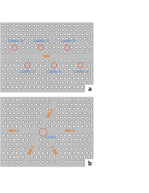
Figure 1: Schematic plots of all-optical circuits incorporating photonic bandgap waveguides and resonators. (a) Many nanocavities couple to one waveguide at different sites; (b) One nanocavity (at the center) couples to many individual waveguides.

The electric and magnetic fields in the photonic network can be expressed in terms of the vector potential $\mathbf{A}(\mathbf{r},t)$ and a scalar potential $\phi(\mathbf{r})$:

$$\mathbf{E}=-\nabla\phi-\frac{1}{c}\frac{\partial\mathbf{A}}{\partial t}\ ,~{}~{}\mathbf{B}=\nabla\times\mathbf{A}\ .$$ (1)

We work in the Coulomb gauge and in the absence of source, which corresponds to the choice of $\phi=0$ with the transversality condition $\nabla\cdot[\epsilon(\mathbf{r})\mathbf{A}(\mathbf{r},t)]=0$. Then the Hamiltonian of the electromagnetic field for the photonic network is given by

$$H=\frac{1}{2}\int d^{3}\mathbf{r}\Big{[}\frac{c^{2}\mathbf{\Pi}(\mathbf{r},t)^{2}}{\epsilon(\mathbf{r})}+(\nabla\times\mathbf{A}(\mathbf{r},t))^{2}\Big{]}\ ,$$ (2)

where $\mathbf{\Pi}(\mathbf{r},t)=\epsilon(\mathbf{r})\dot{\mathbf{A}}(\mathbf{r},t)/c^{2}$ is the canonical conjugate of the vector potential.

We shall expand the vector potential in terms of a complete set of mode functions which are defined by the wave equation

$$\nabla\times[\nabla\times\mathbf{f}_{k}(\mathbf{r})]-\frac{\epsilon(\mathbf{r})\omega^{2}_{k}}{c^{2}}\mathbf{f}_{k}(\mathbf{r})=\mathbf{0}\ ,$$ (3)

where the mode functions $\mathbf{f}_{k}(\mathbf{r})$ satisfy the orthonormality condition

$$\int d^{3}\mathbf{r}\epsilon(\mathbf{r})\mathbf{f}_{k}^{*}(\mathbf{r})\cdot\mathbf{f}_{k^{\prime}}(\mathbf{r})=\delta_{k,k^{\prime}}\ .$$ (4)

Utilizing the Feshbach projection technique FeshbachProj , we separate the whole space of the photonic network by the region $\Im_{i}$ occupied by the cavity $i$, the region $\Im_{\alpha}$ occupied by the waveguides $\alpha$, and the region left denoted by $\Im_{b}$ as the background photonic crystal structure. Because of the presence of the PBG structure, the micro/nano cavities in the photonic crystal have very high $Q$ factor and the loss of the waveguides in the photonic crystal is also extremely low, the field in $\Im_{b}$ is then negligible as an effect of lossless materials for photonic crystals. Consequently, the exact eigenmodes of the vector potential in the photonic network can be decomposed into the eigenmodes in the regions $\Im_{i}$ and $\Im_{\alpha}$, respectively

$$\mathbf{f}_{k}(\mathbf{r})=\sum_{i}\alpha_{i}^{k}\mathbf{u}_{i}(\mathbf{r})+\sum_{\alpha}\sum_{k^{\prime}}\beta_{\alpha k^{\prime}}^{k}\mathbf{v}_{\alpha k^{\prime}}(\mathbf{r})\ ,$$ (5)

where $\mathbf{u}_{i}(\mathbf{r})$ is the eigenmode of cavity $i$, $\mathbf{v}_{\alpha k}(\mathbf{r})$ is the the continuum eigenmode of the waveguide $\alpha$. Both of them form a complete and orthonormal basis set in regions $\Im_{i}$ and $\Im_{\alpha}$ separately. While $\alpha_{i}^{k}$ and $\beta_{\alpha}^{k}$ are the expansion coefficients. The eigenmodes of the cavities and the waveguides satisfy the following equations with the boundary conditions FQ

$$\nabla\times[\nabla \times\mathbf{u}_{i}(\mathbf{r})]-\frac{\epsilon(\mathbf{r})\omega_{i}^{2}}{c^{2}}\mathbf{u}_{i}(\mathbf{r})=\mathbf{0}\ ,$$ (6a)

$$\mathbf{n}\times[\nabla\times\mathbf{u}_{i}(\mathbf{r})]\mid_{\partial\Im_{i}}=\mathbf{0}\ ;$$ (6b)

$$\nabla\times[\nabla \times\mathbf{v}_{\alpha k}(\mathbf{r})]-\frac{\epsilon(\mathbf{r})\omega_{\alpha k}^{2}}{c^{2}}\mathbf{v}_{\alpha k}(\mathbf{r})=\mathbf{0}\ ,$$ (6c)

$$\mathbf{n}\times\mathbf{v}_{\alpha k}(\mathbf{r})\mid_{\partial\Im_{\alpha}}=\mathbf{0}\ .$$ (6d)

With the above decomposition of the exact eigenmodes, we can expand the vector potential of the electromagnetic field in the photonic network and its canonical conjugate in terms of the cavities eigenmodes and the continuous modes of the waveguides

$$\begin{split}&\mathbf{A}(\mathbf{r},t)=\sum_{i}\mathbf{A}_{i}(\mathbf{r},t)+\sum_{\alpha}\mathbf{A}_{\alpha}(\mathbf{r},t)\ ,\\ &\mathbf{\Pi}(\mathbf{r},t)=\sum_{i}\mathbf{\Pi}_{i}(\mathbf{r},t)+\sum_{\alpha}\mathbf{\Pi}_{\alpha}(\mathbf{r},t)\ ,\end{split}$$ (7)

where $\mathbf{A}_{i}(\mathbf{r},t),\mathbf{\Pi}_{i}(\mathbf{r},t)$ and $\mathbf{A}_{\alpha}(\mathbf{r},t),\mathbf{\Pi}_{\alpha}(\mathbf{r},t)$ are vector potential and canonical momentum of the fields in cavity $i$ and waveguide $\alpha$, which can be quantized following the standard quantum field theory in medium. Without the loss of generality and also for simplifying the notation, the photonic network being considered consists of $N$ single mode cavities and $M$ waveguides, each waveguide has a single continuous spectrum (it is indeed straightforward to generalize the result to the case of multi-mode cavities). Then we have

$$\mathbf{A}_{i}(\mathbf{r},t) =c\sqrt{\frac{\hbar}{2\omega_{i}}}~{}\big{[}a_{i}\mathbf{u}_{i}(\mathbf{r})e^{-i\omega_{i}t}+a_{i}^{\dagger}\mathbf{u}^{*}_{i}(\mathbf{r})e^{i\omega_{i}t}\big{]},$$ (8a)

$$\mathbf{\Pi}_{i}(\mathbf{r},t) =-\frac{i\epsilon(\mathbf{r})}{c}\sqrt{\frac{\hbar\omega_{i}}{2}}~{}\big{[}a_{i}\mathbf{u}_{i}(\mathbf{r})e^{-i\omega_{i}t}-a_{i}^{\dagger}\mathbf{u}^{*}_{i}(\mathbf{r})e^{i\omega_{i}t}\big{]},$$ (8b)

$$\mathbf{A}_{\alpha}(\mathbf{r},t) =c\sum_{k}\sqrt{\frac{\hbar}{2\omega_{k}}}~{}\big{[}c_{\alpha k}\mathbf{v}_{\alpha k}(\mathbf{r})e^{-i\omega_{k}t}$$

$$~{}~{}~{}~{}~{}~{}~{}~{}~{}~{}~{}~{}~{}~{}~{}~{}~{}~{}~{}+c^{{\dagger}}_{\alpha k}\mathbf{v}^{*}_{\alpha k}(\mathbf{r})e^{i\omega_{k}t}\big{]},$$ (8c)

$$\mathbf{\Pi}_{\alpha}(\mathbf{r},t) =-\frac{i\epsilon(\mathbf{r})}{c}\sum_{k}\sqrt{\frac{\hbar\omega_{k}}{2}}~{}\big{[}c_{\alpha k}\mathbf{v}_{\alpha k}(\mathbf{r})e^{-i\omega_{k}t}$$

$$~{}~{}~{}~{}~{}~{}~{}~{}~{}~{}~{}~{}~{}~{}~{}~{}~{}~{}~{}~{}~{}~{}~{}~{}~{}~{}~{}-c^{{\dagger}}_{\alpha k}\mathbf{v}^{*}_{\alpha k}(\mathbf{r})e^{i\omega_{k}t}\big{]}\ ,$$ (8d)

where the operators $a_{i},a_{i}^{{\dagger}}$ and $c_{\alpha k},c_{\alpha k}^{{\dagger}}$ are the creation and annihilation operators of the fields in cavity $i$ and waveguide $\alpha$. They obey the following commutation relations

$$[a_{i},a^{{\dagger}}_{j}] =\delta_{ij}\ ,~{}~{}[c_{\alpha k},c^{{\dagger}}_{\alpha^{\prime}k^{\prime}}]=\delta_{\alpha\alpha^{\prime}}\delta_{kk^{\prime}},$$

$$[a_{i},a_{j}] =[c_{\alpha k},c_{\alpha^{\prime}k^{\prime}}]=[a_{i},c_{\alpha k}]=[a^{{\dagger}}_{i},c_{\alpha k}]=0.$$ (9)

Substitute the representations (8) into the Hamiltonian (2), one arrives at the following Hamiltonian for the photonic network

$$H= \sum_{i}\hbar\omega_{i}a^{{\dagger}}_{i}a_{i}+\sum_{\alpha}\sum_{k}\hbar\omega_{k}c^{{\dagger}}_{\alpha k}c_{\alpha k}$$

$$+\hbar\sum_{i}\sum_{\alpha,k}\big{[}V_{i\alpha k}a^{{\dagger}}_{i}c_{\alpha k}+\widetilde{V}_{i\alpha k}a_{i}c_{\alpha k}+{\rm H.c.}\big{]}\ ,$$ (10)

where $V_{i\alpha k}$ and $\widetilde{V}_{i\alpha k}$ are resonant and nonresonant coupling constant between cavities and waveguides which are defined by

$$\begin{split}&V_{i\alpha k}=\frac{c^{2}}{2\sqrt{\omega_{i}\omega_{k}}}\int_{\partial\Im_{i}\cap\partial\Im_{\alpha}}[\mathbf{u}^{*}_{i}(\mathbf{r})\times\mathbf{n}]\cdot[\nabla\times\mathbf{v}_{\alpha k}(\mathbf{r})]\ ,\\ &\tilde{V}_{i\alpha k}=\frac{c^{2}}{2\sqrt{\omega_{i}\omega_{k}}}\int_{\partial\Im_{i}\cap\partial\Im_{\alpha}}[\mathbf{u}_{i}(\mathbf{r})\times\mathbf{n}]\cdot[\nabla\times\mathbf{v}_{\alpha k}(\mathbf{r})]\ .\end{split}$$

Here we have ignored the couplings between cavities and also between different waveguides because their spatial overlaps should be very small. Also, due to the PBG structure in photonic crystals, the features of high $Q$-factor micre/nano cavities and the lossless waveguides allows us to neglect the nonresonant terms. Thus, the Hamiltonian of the photonic network incorporating $M$ photonic bandgap waveguides and $N$ resonators can be rewritten simple as

$$H= \sum_{i=1}^{N}\hbar\omega_{i}a^{{\dagger}}_{i}a_{i}+\sum_{\alpha=1}^{M}\sum_{k}\hbar\omega_{\alpha k}c^{{\dagger}}_{\alpha k}c_{\alpha k}$$

$$~{}~{}~{}~{}+\hbar\sum_{i}\sum_{\alpha,k}\big{(}V_{i\alpha k}a^{{\dagger}}_{i}c_{\alpha k}+H.c.\big{)}\ ,$$ (11)

The explicit form of the cavity and waveguide dispersions, $\omega_{i}$ and $\omega_{\alpha k}$, and the coupling between the cavities and waveguides, $V_{i\alpha k}$, depends on the detailed implementation of the photonic network in photonic crystals, and can be obtained by solving the eigenmode equation (6). It is worth pointing out that the above derivation of the model Hamiltonian can be extended straightforwardly to photonic networks imbedded in other metamaterials.

Furthermore, to control the photonic transport in photonic networks, we must incorporate the external driving fields applying to the cavities and the waveguides, which can be realized by imbedding light emitters such as quantum dot or nanowire to the cavities and the waveguides WGfilter . Then the Hamiltonian is modified as

$$H(t)= \sum_{i}\hbar\omega_{i}a_{i}^{{\dagger}}a_{i}+\sum_{i}\big{(}f_{i}(t)a_{i}^{{\dagger}}+f_{i}^{*}(t)a_{i}\big{)},$$

$$+\sum_{\alpha k}\hbar\omega_{\alpha k}c_{\alpha k}^{\dagger}c_{\alpha k}+\sum_{\alpha k}\big{(}f_{\alpha k}(t)c_{\alpha k}^{{\dagger}}+f_{\alpha k}^{*}(t)c_{\alpha k}\big{)},$$

$$+\hbar\sum_{i\alpha k}\big{(}V_{i\alpha k}(t)a_{i}^{{\dagger}}c_{\alpha k}+V_{i\alpha k}^{*}(t)c_{\alpha k}^{{\dagger}}a_{i}\big{)}.$$ (12a)

This implementation is very similar to the electron transport in mesoscopic systems in nanostructures Hau98 ; Jin10083013 . For the electron transport in mesoscopic systems, one uses bias and gate voltages applying to the electronic leads and the central region to adjust the Fermi surfaces of the leads and the energy levels of the central region. Here one has to use the external driving fields directly acting to the cavities and the waveguides, which leads the Hamiltonian to contain explicitly additional terms proportional to the external driving fields.

Mathematically, we can transfer the external driving field $f_{\alpha k}(t)$ acting on the waveguide $\alpha$ into an equivalent external field acting on the cavities: $f_{i}(t)\rightarrow\tilde{f}_{i}(t)=f_{i}(t)-V_{i\alpha k}(t)f_{\alpha k}(t)/\hbar\omega_{\alpha k}$ through a shift of the waveguide operator $c_{\alpha k}\rightarrow\tilde{c}_{\alpha k}=c_{\alpha k}+f_{\alpha k}(t)/\hbar\omega_{\alpha k}$. Thus the general Hamiltonian for photonic networks can be divided into three parts

$$H(t)=H_{S}(t)+\sum_{\alpha}H_{E\alpha}+\sum_{\alpha}H_{T\alpha}(t)\ ,$$ (13)

where,

$$H_{S}(t)=\sum_{i}\hbar\omega_{i}a_{i}^{{\dagger}}a_{i}+\sum_{i}\big{(}f_{i}(t)a_{i}^{{\dagger}}+f_{i}^{*}(t)a_{i}\big{)}\ ,$$ (14a)

$$H_{E\alpha}=\sum_{k}\hbar\omega_{\alpha k}c_{\alpha k}^{\dagger}c_{\alpha k}\ ,$$ (14b)

$$H_{T\alpha}(t)=\hbar\sum_{ik}\big{(}V_{i\alpha k}(t)a_{i}^{{\dagger}}c_{\alpha k}+V_{i\alpha k}^{*}(t)c_{\alpha k}^{{\dagger}}a_{i}\big{)}\ .$$ (14c)

The first part $H_{S}(t)$ is the Hamiltonian of the cavities in the photonic network plus the contributions of the driving field, $f_{i}(t)$, acting to the cavity $i$ (which also includes the driving field $f_{\alpha k}(t)$ acting on the waveguides in terms of the form of $-V_{i\alpha k}(t)f_{\alpha k}(t)/\omega_{\alpha k}$, as shown above). The second part $H_{E}$ is the Hamiltonian of the waveguides in the photonic network. The third part $H_{T}(t)$ is the coupling between the cavities and the waveguides, which can be time dependent in general through the controls of the coupling between different elements, by means of dynamically tuning the photonic structure manilightPC ; nanomecchannaldrop . With the help of the general Hamiltonian (13), we can model various photonic networks. For the sake of simplicity, we take $\hbar=1$ hereafter.

III Exact master equation for driven resonators

Experimentally, the photonic dynamics of resonators and the photonic transport between waveguides and resonators can be controlled by the external driving field. When a resonator has exchanges of particles, energy and information with the surroundings, it becomes a typical open system. For an open quantum system, its dynamics cannot be properly described by Schrödinger’s wave equation. It should be described by the master equation of the reduced density matrix Car93 . The reduced density matrix of the resonators, denoted by $\rho(t)$, fully depicts the dynamics of photonic coherence of the driven resonators coupled with many waveguides. Any other physical observable is simply given by $\langle O(t)\rangle=\langle O\rho(t)\rangle$.

The reduced density matrix describing the photonic quantum state of the driven resonators is defined by tracing over all of the waveguide degrees of freedom from the total system (the driven resonators plus waveguides):

$$\rho(t)={\rm tr}_{E}[\rho_{\rm tot}(t)]\ ,$$ (15)

where $\rho_{\rm tot}(t)$ is the density matrix of the total system. The total density matrix follows formally the evolution equation:

$$\rho_{\rm tot}(t)=U(t,t_{0})\rho_{\rm tot}(t_{0})U^{{\dagger}}(t,t_{0})\ ,$$ (16)

where $U(t,t_{0})$ is the evolution operator,

$$U(t,t_{0})=T\exp\Big{\{}-i\int_{t_{0}}^{t}H(\tau)d\tau\Big{\}},$$ (17)

in which $T$ is the time-ordering operator, and $H(\tau)$ is the Hamiltonian of the total system given by Eq. (13). In the following, we will derive the exact master equation for the reduced density matrix by explicitly integrating out all of the waveguide degrees of freedom based on the Feynman-Vernon influence functional Fey63118 , similar to the derivation of the master equation for electron coherence dynamics and electron transport in nanostructures Tu08235311 ; Tu09631 ; Jin10083013 and also for a coupled cavity fields in a general bath An07042127 . The difference is that here the system contains external driving fields and the reservoir is at arbitrary finite temperature initially, which makes the derivation much more complicated.

As usual, we assume that there is no initial correlation between the resonators and waveguides Leg871 , namely $\rho_{tot}(t_{0})=\rho(t_{0})\otimes\rho_{E}(t_{0})$, and the waveguides are initially in the equilibrium state, i.e. $\rho_{E}(t_{0})=\frac{1}{Z}e^{-\sum_{\alpha}\beta_{\alpha}H_{E\alpha}}$, with $\beta_{\alpha}=1/(k_{B}T_{\alpha})$ and $T_{\alpha}$ is the initial temperature of the waveguide $\alpha$. Then the reduced density matrix at arbitrary later time $t$ can be expressed in the coherent state representation as An07042127 ; Tu08235311 :

$$\langle\boldsymbol{\alpha}_{f}|\rho(t)|\boldsymbol{\alpha}^{\prime}_{f}\rangle$$

$$=\int d\mu(\boldsymbol{\alpha}_{0})d\mu({\boldsymbol{\alpha}^{\prime}_{0}})\langle\boldsymbol{\alpha}_{0}|\rho(t_{0})|\boldsymbol{\alpha}^{\prime}_{0}\rangle\mathcal{J}(\boldsymbol{\alpha}_{f}^{*},\boldsymbol{\alpha}^{\prime}_{f},t|\boldsymbol{\alpha}_{0},{\boldsymbol{\alpha}^{\prime}}_{0}^{*},t_{0})$$ (18)

with the vector $\boldsymbol{\alpha}=(\alpha_{1},\alpha_{2},...)$ and $|\boldsymbol{\alpha}\rangle=|\alpha_{1}\rangle|\alpha_{2}\rangle...$ is a unnormalized multi-mode coherent states, i.e. $a_{i}|\boldsymbol{\alpha}\rangle=\alpha_{i}|\boldsymbol{\alpha}\rangle$ and $\langle\boldsymbol{\alpha}|\boldsymbol{\alpha}^{\prime}\rangle=\exp(\sum_{i}\alpha^{*}_{i}\alpha^{\prime}_{i})=\exp(\boldsymbol{\alpha}^{\dagger}\boldsymbol{\alpha}^{\prime})$, while $d\mu(\boldsymbol{\alpha})=\frac{d\boldsymbol{\alpha}^{*}d\boldsymbol{\alpha}}{2\pi i}e^{-|\boldsymbol{\alpha}|^{2}}$ is the integral measure of the Bergmann complex space zhang90867 . The propagating function of the reduced density matrix in Eq. (III) is given in terms of path integrals:

$$\mathcal{J}(\boldsymbol{\alpha}_{f}^{*},\boldsymbol{\alpha}^{\prime}_{f},t|\boldsymbol{\alpha}_{0},{\boldsymbol{\alpha}^{\prime}}_{0}^{*},t_{0})$$

$$=\int{\cal D}[\boldsymbol{\alpha}^{*}\boldsymbol{\alpha};{\boldsymbol{\alpha}^{\prime}}^{*}\boldsymbol{\alpha}^{\prime}]e^{i(S_{S}[\boldsymbol{\alpha}^{*},\boldsymbol{\alpha}]-S_{S}[{\boldsymbol{\alpha}^{\prime}}^{*},\boldsymbol{\alpha}^{\prime}])}\mathscr{F}[\boldsymbol{\alpha}^{*}\boldsymbol{\alpha};{\boldsymbol{\alpha}^{\prime}}^{*}\boldsymbol{\alpha}^{\prime}]$$ (19)

with the integral boundary conditions: $\boldsymbol{\alpha}(t_{0})=\boldsymbol{\alpha}_{0}$, $\boldsymbol{\alpha}^{*}(t)=\boldsymbol{\alpha}_{f}^{*}$, ${\boldsymbol{\alpha}^{\prime}}^{*}(t_{0})={\boldsymbol{\alpha}^{\prime}}_{0}^{*}$, and $\boldsymbol{\alpha}^{\prime}(t)=\boldsymbol{\alpha}^{\prime}_{f}$, where $S_{S}[\boldsymbol{\alpha}^{*},\boldsymbol{\alpha}]$ is the action of the driven resonators in the coherent state representation:

$$S_{S}[\boldsymbol{\alpha}^{*},\boldsymbol{\alpha}]= -\frac{i}{2}[\boldsymbol{\alpha}^{{\dagger}}_{f}\boldsymbol{\alpha}(t)+\boldsymbol{\alpha}^{{\dagger}}(t_{0})\boldsymbol{\alpha}_{0}]+\int_{t_{0}}^{t}d\tau\Big{\{}\frac{i}{2}\Big{[}\boldsymbol{\alpha}^{{\dagger}}\frac{d\boldsymbol{\alpha}}{d\tau}$$

$$-\frac{d\boldsymbol{\alpha}^{{\dagger}}}{d\tau}\boldsymbol{\alpha}\Big{]}-(\boldsymbol{\alpha}^{{\dagger}}\boldsymbol{\omega}\boldsymbol{\alpha}+\boldsymbol{\alpha}^{{\dagger}}\boldsymbol{f}+\boldsymbol{f}^{{\dagger}}\boldsymbol{\alpha})\Big{\}},$$ (20)

in which the frequency matrix $\boldsymbol{\omega}\equiv\{\omega_{ij}\}$ (here the off-diagonal matrix elements representing the possible couplings between different cavities are included for the generality of the formulation) and the driving field vector $\boldsymbol{f}(\tau)\equiv\{f_{i}(\tau)\}$. While $\mathscr{F}[\boldsymbol{\alpha}^{*}\boldsymbol{\alpha};\boldsymbol{\alpha}^{\prime*}\boldsymbol{\alpha}^{\prime}]$ is the influence functional Fey63118 obtained after integrated out all of the waveguide degrees of freedom An07042127 ; Tu08235311 :

$$\mathscr{F}[\boldsymbol{\alpha}^{*} \boldsymbol{\alpha};{\boldsymbol{\alpha}^{\prime}}^{*}\boldsymbol{\alpha}^{\prime}]=\exp\Big{\{}\sum_{\alpha}(-\int_{t_{0}}^{t}d\tau\int_{t_{0}}^{\tau}d\tau^{\prime}\boldsymbol{\alpha}^{{\dagger}}(\tau)\mathbf{g}_{\alpha}(\tau,\tau^{\prime})\boldsymbol{\alpha}(\tau^{\prime})-\int_{t_{0}}^{t}d\tau\int_{t_{0}}^{\tau}d\tau^{\prime}\boldsymbol{\alpha}^{\prime{\dagger}}(\tau^{\prime})\mathbf{g}_{\alpha}(\tau^{\prime},\tau)\boldsymbol{\alpha}^{\prime}(\tau)$$

$$+\int_{t_{0}}^{t}d\tau\int_{t_{0}}^{t}d\tau^{\prime}{\boldsymbol{\alpha}^{\prime}}^{{\dagger}}(\tau)\mathbf{g}_{\alpha}(\tau,\tau^{\prime})\boldsymbol{\alpha}(\tau^{\prime})-\int_{t_{0}}^{t}d\tau\int_{t_{0}}^{t}d\tau^{\prime}[\boldsymbol{\alpha}^{{\dagger}}(\tau)-{\boldsymbol{\alpha}^{\prime}}^{{\dagger}}(\tau)]\widetilde{\mathbf{g}}_{\alpha}(\tau,\tau^{\prime})[\boldsymbol{\alpha}(\tau^{\prime})-\boldsymbol{\alpha}^{\prime}(\tau^{\prime})])\Big{\}}.$$ (21)

The time-correlation functions in Eq. (III) are given by:

$$\mathbf{g}_{\alpha ij}(\tau,\tau^{\prime}) =\sum_{k}V_{i\alpha k}(\tau)V_{j\alpha k}^{*}(\tau^{\prime})e^{-i\omega_{\alpha k}(\tau-\tau^{\prime})}\ ,$$ (22a)

$$\widetilde{\mathbf{g}}_{\alpha ij}(\tau,\tau^{\prime}) =\sum_{k}V_{i\alpha k}(\tau)V_{j\alpha k}^{*}(\tau^{\prime})n_{\alpha}(\omega_{\alpha k})e^{-i\omega_{\alpha k}(\tau-\tau^{\prime})},$$ (22b)

which depict the time correlations of photons in the waveguides through the resonators, and $n_{\alpha}(\omega_{\alpha k})=1/(e^{\beta_{\alpha}\omega_{\alpha k}}-1)$ is the initial thermal photonic distribution function in the waveguide $\alpha$ at the time $t_{0}$. The influence functional, Eq. (III), contains all the back reactions from waveguides to the driven resonators through the photonic transfer between the resonators and waveguides. If the coupling constants do not explicitly depend on the time, then introducing the spectral density $J_{\alpha}(\omega)=2\pi\sum_{k}V_{i\alpha k}V_{j\alpha k}^{*}\delta(\omega-\omega_{\alpha k})$, we can simply express the time-correlation function in terms of the spectral density as follows

$$\mathbf{g}_{\alpha ij}(\tau,\tau^{\prime}) =\int\frac{d\omega}{2\pi}J_{\alpha}(\omega)e^{-i\omega(\tau-\tau^{\prime})}\ ,$$ (23a)

$$\widetilde{\mathbf{g}}_{\alpha ij}(\tau,\tau^{\prime}) =\int\frac{d\omega}{2\pi}J_{\alpha}(\omega)n_{\alpha}(\omega)e^{-i\omega(\tau-\tau^{\prime})}\ .$$ (23b)

As shown in Eqs. (III) and (III), after integrated out all of the waveguide degrees of freedom, the effective action in the propagating function remains in a quadratic form. Therefore, the path integral in the propagating function can be carried out exactly through the stationary path method. The resulting propagating function, Eq. (III), becomes (see a detailed derivation given in Appendix A)

$$\mathcal{J}( \boldsymbol{\alpha}^{*}_{f},\boldsymbol{\alpha}^{\prime}_{f},t|\boldsymbol{\alpha}_{0},{\boldsymbol{\alpha}^{\prime}}_{0}^{*},t_{0})=A(t)\exp\{(\boldsymbol{\alpha}^{{\dagger}}_{f}-\boldsymbol{y}^{{\dagger}}(t))\boldsymbol{J}_{1}(t)\boldsymbol{\alpha}_{0}$$

$$+{\boldsymbol{\alpha}^{\prime}}_{0}^{{\dagger}}\boldsymbol{J}_{1}^{{\dagger}}(t)(\boldsymbol{\alpha}^{\prime}_{f}-\boldsymbol{y}(t))+\boldsymbol{\alpha}^{{\dagger}}_{f}\boldsymbol{J}_{2}(t)\boldsymbol{\alpha}^{\prime}_{f}+{\boldsymbol{\alpha}^{\prime}}^{{\dagger}}_{0}\boldsymbol{J}_{3}(t)\boldsymbol{\alpha}_{0}$$

$$-\boldsymbol{\alpha}^{{\dagger}}_{f}\boldsymbol{y}(t)-\boldsymbol{y}^{{\dagger}}(t)\boldsymbol{\alpha}^{\prime}_{f}-\boldsymbol{y}^{{\dagger}}(t)\boldsymbol{w}(t)\boldsymbol{y}(t)\},$$ (24)

in which $A(t)=\det[\boldsymbol{w}(t)]$, $\boldsymbol{J}_{1}(t)=\boldsymbol{w}(t)\boldsymbol{u}(t,t_{0})$, $\boldsymbol{J}_{2}(t)=1-\boldsymbol{w}(t)$, $\boldsymbol{J}_{3}(t)=1-\boldsymbol{u}^{{\dagger}}(t,t_{0})\boldsymbol{w}(t)\boldsymbol{u}(t,t_{0})$ and $\boldsymbol{w}(t)=[\boldsymbol{1}+\boldsymbol{v}(t,t)]^{-1}=\boldsymbol{w}^{{\dagger}}(t)$. The function $\boldsymbol{u}(\tau,t_{0})$, $\bar{\boldsymbol{u}}(\tau,t)$, $\boldsymbol{v}(\tau,t)$ are $N$ by $N$ matrices, and $\boldsymbol{y}(t)$ is a $1\times N$ matrix, where $N$ is the number of resonator modes. These functions obey the equations of motion

$$\frac{d\boldsymbol{u}(\tau,t_{0})}{d\tau}+i\boldsymbol{\omega}\boldsymbol{u}(\tau,t_{0})+\int_{t_{0}}^{\tau}\mathbf{g}(\tau,\tau^{\prime})\boldsymbol{u}(\tau^{\prime},t_{0})d\tau^{\prime}=0\ ,$$ (25a)

$$\frac{d\bar{\boldsymbol{u}}(\tau,t)}{d\tau}+i\boldsymbol{\omega}\bar{\boldsymbol{u}}(\tau,t)-\int_{\tau}^{t}\mathbf{g}(\tau,\tau^{\prime})\bar{\boldsymbol{u}}(\tau^{\prime},t)d\tau^{\prime}=0\ ,$$ (25b)

$$\frac{d\boldsymbol{v}(\tau,t)}{d\tau}+i\boldsymbol{\omega}\boldsymbol{v}(\tau,t)+\int_{t_{0}}^{\tau}\mathbf{g}(\tau,\tau^{\prime})\boldsymbol{v}(\tau^{\prime},t)d\tau^{\prime}$$

$$~{}~{}~{}~{}~{}~{}~{}~{}~{}~{}~{}~{}~{}~{}~{}~{}~{}~{}~{}~{}~{}~{}~{}~{}~{}~{}~{}~{}~{}~{}=\int_{t_{0}}^{t}\widetilde{\mathbf{g}}(\tau,\tau^{\prime})\bar{\boldsymbol{u}}(\tau^{\prime},t)d\tau^{\prime}\ ,$$ (25c)

$$\frac{d\boldsymbol{y}(\tau)}{d\tau}+i\boldsymbol{\omega}\boldsymbol{y}(\tau)+\int_{t_{0}}^{\tau}\mathbf{g}(\tau,\tau^{\prime})\boldsymbol{y}(\tau^{\prime})d\tau^{\prime}=-i\boldsymbol{f}(\tau)$$ (25d)

subjected to the initial conditions $\bar{\boldsymbol{u}}(t,t)=1$, $\boldsymbol{u}(t_{0},t_{0})=1$, $\boldsymbol{v}(t_{0},t)=0$ and $\boldsymbol{y}(t_{0})=0$ with $t_{0}\leq\tau,\tau^{\prime}\leq t$. Here we have also defined $\mathbf{g}(\tau,\tau^{\prime})=\sum_{\alpha}\mathbf{g}_{\alpha}(\tau,\tau^{\prime})$ and $\widetilde{\mathbf{g}}(\tau,\tau^{\prime})=\sum_{\alpha}\widetilde{\mathbf{g}}_{\alpha}(\tau,\tau^{\prime})$. It is not too difficult to find that

$$\bar{\boldsymbol{u}}(\tau,t)=\boldsymbol{u}^{{\dagger}}(t,\tau)\ ,$$ (26a)

$$\boldsymbol{y}(\tau)=-i\int_{t_{0}}^{\tau}\boldsymbol{u}(\tau,\tau^{\prime})\boldsymbol{f}(\tau^{\prime})d\tau^{\prime}\ ,$$ (26b)

$$\boldsymbol{v}(\tau,t)=\int_{t_{0}}^{\tau}d\tau^{\prime}\int_{t_{0}}^{t}d\tau^{\prime\prime}\boldsymbol{u}(\tau,\tau^{\prime})\widetilde{\mathbf{g}}(\tau^{\prime},\tau^{\prime\prime})\bar{\boldsymbol{u}}(\tau^{\prime\prime},t)\ .$$ (26c)

As we see, once Eq. (25a) is solved for $\boldsymbol{u}(\tau,t_{0})$, the dynamics of the driven resonators can be completely determined.

Substituting Eq. (III) into Eq. (III), taking a time derivative to the reduced density matrix, and then using the relations zhang90867 : $a_{i}|\boldsymbol{\alpha}\rangle=\alpha_{i}|\boldsymbol{\alpha}\rangle$ and $\frac{\partial}{\partial\alpha_{i}}|\boldsymbol{\alpha}\rangle=a_{i}^{{\dagger}}|\boldsymbol{\alpha}\rangle$, we obtain a time convolutionless but exact master equation for the driving resonator system coupled to waveguides:

$$\frac{d\rho(t)}{dt}=-i[H_{\rm eff}(t),\rho(t)]$$

$$+\sum_{ij}\gamma_{ij}(t)[2a_{j}\rho(t)a_{i}^{{\dagger}}-\rho(t)a_{i}^{{\dagger}}a_{j}-a_{i}^{{\dagger}}a_{j}\rho(t)]$$

$$+\sum_{ij}\widetilde{\gamma}_{ij}(t)[a_{j}\rho(t)a_{i}^{{\dagger}}+a_{i}^{{\dagger}}\rho(t)a_{j}-a_{i}^{{\dagger}}a_{j}\rho(t)-\rho(t)a_{j}a_{i}^{{\dagger}}],$$ (27)

where $H_{\rm eff}(t)=\sum_{ij}\omega_{ij}^{\prime}(t)a^{{\dagger}}_{i}a_{j}+\sum_{i}[f^{\prime}_{i}(t)a^{{\dagger}}_{i}+{f^{\prime}}_{i}^{*}(t)a_{i}]$ is the effective Hamiltonian of the driven resonators. The renormalized frequencies $\omega_{ij}^{\prime}(t)$ and the renormalized driving field $f^{\prime}_{i}(t)$ result from the back-reaction effect of the waveguides coupled to the resonators. The initial temperature effects are fully incorporated into the temperature-dependent noise coefficient $\widetilde{\boldsymbol{\gamma}}(t)$. The time dependent dissipation coefficients $\boldsymbol{\gamma}$(t) together with the time-dependent noise coefficients $\widetilde{\boldsymbol{\gamma}}(t)$ describe the non-Markovian dissipation and decoherence dynamics of the resonators due to the interaction between the resonators and waveguides. Here these coefficients also describe the photon transport from the resonators into the waveguides under the control of external driving fields, as we will show in the next section. All these time-dependent coefficients in Eq. (III) are given explicitly as follow:

$$\omega^{\prime}_{ij}(t) =\omega_{ij}(t)-\frac{i}{2}\sum_{\alpha}[\boldsymbol{\kappa}_{\alpha}(t)-\boldsymbol{\kappa}_{\alpha}^{{\dagger}}(t)]_{ij}\ ,$$ (28a)

$$\gamma_{ij}(t) =\frac{1}{2}\sum_{\alpha}[\boldsymbol{\kappa}_{\alpha}(t)+\boldsymbol{\kappa}_{\alpha}^{{\dagger}}(t)]_{ij}\ ,$$ (28b)

$$\widetilde{\gamma}_{ij}(t) =\sum_{\alpha}[\boldsymbol{\lambda}_{\alpha}(t)+\boldsymbol{\lambda}_{\alpha}^{{\dagger}}(t)]_{ij}\ ,$$ (28c)

$$f^{\prime}_{i}(t) =f_{i}(t)+\sum_{\alpha}[\boldsymbol{f}_{\alpha}(t)]_{i}$$ (28d)

with

$$\boldsymbol{\kappa}_{\alpha}(t) =\int_{t_{0}}^{t}d\tau\mathbf{g}_{\alpha}(t,\tau)\boldsymbol{u}(\tau,t_{0})\boldsymbol{u}^{-1}(t,t_{0})\ ,$$ (29a)

$$\boldsymbol{\lambda}_{\alpha}(t) =\int_{t_{0}}^{t}d\tau[\mathbf{g}_{\alpha}(t,\tau)\boldsymbol{v}(\tau,t)-\widetilde{\mathbf{g}}_{\alpha}(t,\tau)\bar{\boldsymbol{u}}(\tau,t)]$$

$$~{}~{}~{}~{}~{}~{}~{}~{}~{}~{}~{}~{}~{}~{}~{}-\boldsymbol{\kappa}_{\alpha}(t)\boldsymbol{v}(t,t)\ ,$$ (29b)

$$\boldsymbol{f}_{\alpha}(t) =i\boldsymbol{\kappa}_{\alpha}(t)\boldsymbol{y}(t)-i\int_{t_{0}}^{t}d\tau\mathbf{g}_{\alpha}(t,\tau)\boldsymbol{y}(\tau)$$ (29c)

as functions of $\boldsymbol{u}(t,t_{0})$, $\boldsymbol{v}(t,t)$ and $\boldsymbol{y}(t)$ that are determined by the integrodifferential equations of Eq. (25). We should point out that although it has a time convolutionless form, the master equation is exact and the non-Markovian memory effect between the resonators and waveguides is fully embodied non-perturbatively in the integral kernels involving the non-local time-correlation functions of the waveguides, $\mathbf{g}(\tau,\tau^{\prime})$ and $\widetilde{\mathbf{g}}(\tau,\tau^{\prime})$, in Eq. (25). We should also point out that $\boldsymbol{f}_{\alpha}(t)$ is a shift to the external driving field $\boldsymbol{f}(t)$, which comes from the back-reaction of the waveguide $\alpha$ to the resonators. In other words, $\boldsymbol{f}_{\alpha}(t)$ is a feed-back effect to the external driving field. We may call the function $\boldsymbol{y}(t)$ (see Eq. (26b)) as the driving-induced field.

Notice that using the Feynman-Vernon influence functional approach to derive the exact master equation was carried out early for quantum Brown motion (QBM) Hu922843 ; Kar97153 . The exact master equation can also be obtained by the trace-over-bath on total-space Wigner-function method Haa852462 ; Hal962012 ; For01105020 or the stochastic diffusion Schrödinger equation Str04052115 . All these previous works deal mainly with a single harmonic oscillator coupled to a thermal bath without external driving fields. The extension of the exact master equation to the systems of two entangled optical modes or two entangled harmonic oscillators has only been worked out very recently An07042127 ; Cho08011112 ; Paz08220401 . The exact master equation of Eq. (III) obtained here is indeed the most general one for the system containing arbitrary number of entangled modes coupled to arbitrary number of photonic reservoirs with arbitrary spectral density at arbitrary initial temperatures under arbitrary number of external driving fields. It allows to investigate various general and exact non-Markovian dynamics in photonic systems.

On the other hands, one may obtain a time-convolutionless master equation from perturbation expansion up to the second order in terms of the coupling constant between the system and the reservoir Bre02 ; Car93 . Such a time-convolutionless master equation is valid only in the weak coupling regime where the non-Markovian effect is also very weak, except for some structured reservoirs switching . Also, the time-convolutionless perturbation master equation up to the second order in the system-reservoir coupling is indeed the same as the Born-Markov master equation without taking the long time limit Car93 ; Xio10012105 . An exception of the time convolutionless exact master equation not for pure optical systems is the master equation of a two-level atom with one single photon at zero temperature Bre991633 ; An10052330 . However, when the number of photons increases, the problem becomes intractable and the general non-Markovian dynamics with arbitrary number of photons at arbitrary temperature has not been well explored in quantum optics. Different from the study on the non-Markovian atomic dynamics involving only one single photon in quantum optics, the exact master equation of Eq. (III) is capable to investigate the general and the exact non-Markovian process involving arbitrary number of photons of the reservoir with arbitrary spectral density at arbitrary temperature in all-optical circuits. Applications to such exact non-Markovian dynamics of a micro/nano cavity coupled to a general thermal reservoir and a structured reservoir in photonic crystals have just been worked out very recently Xio10012105 ; Wu1018407 .

In fact, the master equation (III) determines all the nonequilibrium dynamics of the driven resonators and the photonic transport between the resonators and the waveguides in photonic networks. The aim of the present paper is to use the exact master equation derived above to establish a quantum transport theory that generalizes the quantum transport theory based on the Keldysh’s nonequilibrium Green function technique. We will show in the next section how the photocurrent passing through the resonators into waveguides can be obtained directly from the master equation, and how the quantum transport theory based on the Keldysh’s nonequilibrium Green function technique can be easily reproduced and generalized. Before end this section, we shall calculate some important physical observables describing the photonic dynamics in the driven resonators. One of them is the time evolution of the photonic resonator field, and another one is the single particle reduced density matrix which characterizes photonic intensity of the resonators. These are two main quantities related to the non-Markovian transport dynamics in photonic systems.

The photonic field of the resonators is determined by $\langle a_{i}(t)\rangle={\rm tr}_{s}[a_{i}\rho(t)]$. With the help of the master equation, it obeys the equation of motion:

$$\frac{d}{dt}\langle a_{i}(t)\rangle=\sum_{j}[\dot{\boldsymbol{u}}(t,t_{0})\boldsymbol{u}^{-1}(t,t_{0})]_{ij}\langle a_{j}(t)\rangle-if^{\prime}_{i}(t)\ .$$ (30)

Its solution is:

$$\langle a_{i}(t)\rangle=\sum_{j}u_{ij}(t,t_{0})\langle a_{j}(t_{0})\rangle+y_{i}(t)\ .$$ (31)

In other words, the photonic field of the driven resonators is a combination of the photonic propagating of the initial field $\boldsymbol{u}(t,t_{0})\langle a_{j}(t_{0})\rangle$ and the driving-induced field $\boldsymbol{y}(t)$ (see Eq. (26b)). This solution describes the driving-field-induced photonic coherence in resonators. Similarly, the equation of motion for the single particle reduced density matrix of the resonators, $\rho^{(1)}_{ij}(t)={\rm tr}_{s}[a^{{\dagger}}_{j}a_{i}\rho(t)]$, can also be found from the exact master equation:

$$\frac{d}{dt}\rho^{(1)}_{ij}(t)=\sum_{m}\{[\dot{\boldsymbol{u}}(t,t_{0})\boldsymbol{u}^{-1}(t,t_{0})]_{im}\rho^{(1)}_{mj}(t)$$

$$+\rho^{(1)}_{im}(t)[\dot{\boldsymbol{u}}(t,t_{0})\boldsymbol{u}^{-1}(t,t_{0})]^{{\dagger}}_{mj}\}+\widetilde{\gamma}_{ij}(t)$$

$$-if^{\prime}_{i}(t)\langle a^{{\dagger}}_{j}(t)\rangle+i\langle a_{i}(t)\rangle{f^{\prime}_{j}}^{{\dagger}}(t)\ .$$ (32)

The solution of the above equation of motion can also be obtained explicitly in terms of the functions $\boldsymbol{u}(t,t_{0})$, $\boldsymbol{v}(t,t)$ and the driving-induced field $\boldsymbol{y}(t)$:

$$\rho^{(1)}_{ij}(t)=\sum_{mn}u_{im}(t,t_{0})\rho^{(1)}_{mn}(t_{0})u^{*}_{ni}(t,t_{0})+v_{ij}(t,t)$$

$$+\langle a_{i}(t)\rangle y^{*}_{j}(t)+y_{i}(t)\langle a^{{\dagger}}_{j}(t)\rangle\ -y_{i}(t)y^{*}_{j}(t).$$ (33)

The first term in the above solution comes from the initial photonic distribution in the resonators. The second term is the effect induced by the thermal fluctuation in the waveguides (see the solution of $\boldsymbol{v}(t,t)$ by Eq. (26c)). The remaining terms are the contribution coming from the driving fields. Besides, the $i$th diagonal element of the single particle reduced density matrix gives the average photon number of the mode $i$ in the resonators, i.e.

$$\rho^{(1)}_{ii}(t)={\rm tr}_{s}[a^{{\dagger}}_{i}a_{i}\rho(t)]=n_{i}(t),$$ (34)

which measures the photonic intensity of the $i$th mode in the resonators. The photonic coherence and the photonic intensity of the driven resonators, given respectively by Eqs. (31) and (34), play the important role for the photonic transport in photonic networks, as we shall discuss in the next section.

IV Photonic transport in photonic networks

In this section, we are going to derive the exact photocurrent flowing from the resonators into each waveguide. Connection between the photocurrent and the master equation of the reduced density matrix is given, which explicitly demonstrates the intimacy between quantum coherence and quantum transport in nonequilibrium dynamics. Also, the relation between the transport theory obtained here with the transport theory based on the Keldysh’s nonequilibrium Green function technique is discussed and the powerfulness of the present theory is given.

IV.1 Photocurrent in each waveguide channel

To find the photocurrent flowing from the resonators to each waveguide using the master equation, it will be more convenient to reexpress the master equation, Eq. (III), as follows:

$$\frac{d\rho(t)}{dt}=-i[H_{S}(t),\rho(t)]+\sum_{\alpha}[\mathcal{L}_{\alpha}^{+}(t)+\mathcal{L}_{\alpha}^{-}(t)]\rho(t)\ .$$ (35)

Here $H_{S}(t)$ is the original Hamiltonian of Eq. (14a) for the driven resonators. $\mathcal{L}_{\alpha}^{+}(t)$ and $\mathcal{L}_{\alpha}^{-}(t)$ are superoperators acting on the reduced density matrix, induced by the coupling to the waveguides. They are given by:

$$\mathcal{L}_{\alpha}^{+}(t) \rho(t)=\sum_{ij}\{\lambda_{\alpha ij}(t)[a_{j}\rho(t)a^{{\dagger}}_{i}-\rho(t)a_{j}a^{{\dagger}}_{i}]$$

$$-\kappa_{\alpha ij}(t)a^{{\dagger}}_{i}a_{j}\rho(t)-if_{\alpha i}(t)a_{i}^{{\dagger}}\rho(t)+{\rm H.c.}\}\ ,$$ (36a)

$$\mathcal{L}_{\alpha}^{-}(t) \rho(t)=\sum_{ij}\{\lambda_{\alpha ij}(t)[a^{{\dagger}}_{i}\rho(t)a_{j}-a^{{\dagger}}_{i}a_{j}\rho(t)]$$

$$+\kappa_{\alpha ij}(t)a_{j}\rho(t)a^{{\dagger}}_{i}+if_{\alpha i}(t)\rho(t)a_{i}^{{\dagger}}+{\rm H.c.}\}$$ (36b)

The superoperators $\mathcal{L}_{\alpha}^{+}(t)$ and $\mathcal{L}_{\alpha}^{-}(t)$ are intimately related to the photocurrent through the waveguide $\alpha$, as we will see next.

The photocurrent flowing from the resonators into the waveguide $\alpha$ is defined in the Heisenberg picture as:

$$I_{\alpha}(t) \equiv\frac{d\langle N_{\alpha}(t)\rangle}{dt}=-i\langle[N_{\alpha}(t),H(t)]\rangle$$

$$=i\sum_{ki}[V_{i\alpha k}(t)\langle a^{{\dagger}}_{i}(t)c_{\alpha k}(t)\rangle-V^{*}_{i\alpha k}(t)\langle a^{{\dagger}}_{i}(t)c_{\alpha k}(t)\rangle]\ ,$$ (37)

where $N_{\alpha}=\sum_{k}c^{\dagger}_{\alpha k}c_{\alpha k}$ is the photon number operator of the waveguide $\alpha$. Furthermore, consider the single particle reduced density matrix in the Heisenberg picture: $\rho^{(1)}_{ij}(t)={\rm tr}_{s}[a^{{\dagger}}_{j}a_{i}\rho(t)]=\langle a^{{\dagger}}_{j}(t)a_{i}(t)\rangle$, we find that

$$\frac{d\boldsymbol{\rho}^{(1)}(t)}{dt}=-i[\boldsymbol{\omega},\boldsymbol{\rho}^{(1)}(t)]+\boldsymbol{\cal S}(t)-\sum_{\alpha}\boldsymbol{\cal I}_{\alpha}(t)\ ,$$ (38)

where $\boldsymbol{\cal I}_{\alpha}(t)$ and $\boldsymbol{\cal S}(t)$ are the current matrix of the waveguide $\alpha$ and the source matrix of the driven resonators:

$${\cal S}_{ij}(t) =i\langle a_{i}(t)\rangle f^{*}_{j}(t)-if_{i}(t)\langle a^{{\dagger}}_{j}(t)\rangle\ ,$$ (39a)

$${\cal I}_{\alpha ij}(t) =i\sum_{k}[V_{i\alpha k}(t)\langle a^{{\dagger}}_{j}(t)c_{\alpha k}(t)\rangle-V^{*}_{j\alpha k}(t)\langle a^{{\dagger}}_{i}(t)c_{\alpha k}\rangle].$$ (39b)

Comparing Eqs. (IV.1) and (39b), one can see that the trace of the current matrix is just the photocurrent flowing from the resonators into the waveguide $\alpha$: $I_{\alpha}(t)={\rm Tr}[\boldsymbol{\cal I}_{\alpha}(t)]$. Note that ${\rm Tr}$ is the trace over the $N\times N$ matrix of the $N$ single modes in the resonators, while ${\rm tr}_{s}$ and ${\rm tr}_{E}$ used before denote the traces over all the quantum states of the resonators and the waveguides, respectively.

On the other hand, the equation of motion for the single particle reduced density matrix can also be obtained directly from the master equation, Eq. (35). The result is

$$\frac{d}{dt}\rho^{(1)}_{ij}(t)= -i[\boldsymbol{\omega},\boldsymbol{\rho}^{(1)}(t)]_{ij}+S_{ij}(t)$$

$$+\sum_{\alpha}{\rm tr}_{s}[a^{{\dagger}}_{j}a_{i}[\mathcal{L}^{+}_{\alpha}(t)+\mathcal{L}^{-}_{\alpha}(t)]\rho(t)]\ .$$ (40)

Comparing Eqs. (38) and (IV.1) for the single particle reduced density matrix, with the help of Eqs. (36) and (29), we obtain the explicit formula for the photocurrent matrix:

$$\boldsymbol{\cal I}_{\alpha}(t)=\int_{t_{0}}^{t}d\tau\big{\{}\mathbf{g}_{\alpha}(t,\tau)\boldsymbol{\rho}^{(1)}(\tau,t)-\widetilde{\mathbf{g}}_{\alpha}(t,\tau)\bar{\boldsymbol{u}}(\tau,t)+{\rm H.c.}\big{\}}$$ (41)

and $\boldsymbol{\rho}^{(1)}(\tau,t)$ is the generalized correlation function which is given explicitly by:

$$\rho^{(1)}_{ij}(\tau,t) =\sum_{mn}u_{im}(\tau,t_{0})\rho^{(1)}_{mn}(t_{0})u^{*}_{ni}(t,t_{0})+v_{ij}(\tau,t)$$

$$+y_{i}(\tau)y^{*}_{j}(t)+\sum_{m}[u_{im}(\tau,t_{0})\langle a_{m}(t_{0})\rangle y^{*}_{j}(t)$$

$$~{}~{}~{}~{}~{}~{}~{}~{}+y_{i}(\tau)\langle a^{{\dagger}}_{m}(t_{0})\rangle u^{*}_{mj}(t,t_{0})]\ .$$ (42)

Then the photocurrent flowing into the waveguide $\alpha$ is simply given by:

$$I_{\alpha}(t)=2{\rm Re}{\int_{t_{0}}^{t}d\tau{\rm Tr}[\mathbf{g}_{\alpha}(t,\tau)\boldsymbol{\rho}^{(1)}(\tau,t)-\widetilde{\mathbf{g}}_{\alpha}(t,\tau)\bar{\boldsymbol{u}}(\tau,t)]}.$$ (43)

It shows that the photocurrent is completely determined by the time-correlation functions $\mathbf{g}_{\alpha}(t,\tau)$ and $\widetilde{\mathbf{g}}_{\alpha}(t,\tau)$ of the waveguides and the propagating and correlation functions $\bar{\boldsymbol{u}}(\tau,t)$ and $\boldsymbol{\rho}^{(1)}(\tau,t)$ of the driven resonators. The time-correlation functions characterize the non-Markovian memory structure of photon transfer between resonators and waveguides, while the propagating and correlation functions depict completely the photon coherence and photon correlation of the resonators under the control of external driving fields.

In fact, Eq. (38) is a generalized quantum continuous equation. By tracing over the equation of motion for the single particle reduced density matrix, we have

$$\frac{dN}{dt}=S(t)-\sum_{\alpha}I_{\alpha}(t)\ .$$ (44)

Here $N(t)={\rm Tr}[\boldsymbol{\rho}^{(1)}(t)]$ is the total photon number in the resonators, $S(t)={\rm Tr}[\boldsymbol{\cal S}(t)]$ is the source coming from the driving fields, and $I_{\alpha}(t)={\rm Tr}[\boldsymbol{\cal I}_{\alpha}(t)]$ is the photocurrent flowing into the waveguides $\alpha$. Eq. (44) tells that the increase of the photon number in the resonators equals to the receiving photons from the driving field subtracting the lessening photons flowing into waveguides.

IV.2 Relations to the Keldysh’s nonequilibrium Green function technique

As one seen from Eq. (43), the photocurrent is completely determined by the time-correlation functions $\mathbf{g}_{\alpha}(t,\tau)$ and $\widetilde{\mathbf{g}}_{\alpha}(t,\tau)$ of the waveguides plus the propagating and correlation functions $\bar{\boldsymbol{u}}(\tau,t)$ and $\boldsymbol{\rho}^{(1)}(\tau,t)$ of the driven resonators. In fact, we have shown Jin10083013 that the functions $\boldsymbol{u}(\tau,t_{0})$, $\bar{\boldsymbol{u}}(\tau,t)$, $\boldsymbol{\rho}^{(1)}(\tau,t)$ are related to the retarded, advanced and lesser Green functions of the resonators in the Keldysh’s nonequilibrium formulism Sch61407 ; Cho851 ; Hau98 :

$$u_{ij}(t_{1},t_{2})=\theta(t_{1}-t_{2})\langle[a_{i}(t_{1}),a^{\dagger}_{j}(t_{2})]\rangle\equiv iG^{r}_{ij}(t_{1},t_{2}),$$ (45a)

$$\bar{u}_{ij}(t_{1},t_{2})=\theta(t_{2}-t_{1})\langle[a_{i}(t_{1}),a^{\dagger}_{j}(t_{2})]\rangle\equiv-iG^{a}_{ij}(t_{1},t_{2}),$$ (45b)

$$\rho^{(1)}_{ij}(t_{1},t_{2})=\langle a^{\dagger}_{j}(t_{2})a_{i}(t_{1})\rangle\equiv-iG^{<}_{ij}(t_{1},t_{2}).$$ (45c)

While, the time-correlation functions $\mathbf{g}_{\alpha}(t,\tau)$ and $\widetilde{\mathbf{g}}_{\alpha}(t,\tau)$ correspond to the retarded and lesser self-energy functions arose from the couplings between the resonators and the waveguides:

$$\mathbf{g}_{\alpha ij}(t_{1},t_{2})=i\Sigma^{r}_{\alpha ij}(t_{1},t_{2}),$$ (46a)

$$\widetilde{\mathbf{g}}_{\alpha ij}(t_{1},t_{2})=-i\Sigma^{<}_{\alpha ij}(t_{1},t_{2}).$$ (46b)

The explicit form of these self-energy functions is given by Eq. (22) or (23) which is rather simple. In the Keldysh’s nonequilibrium Green function technique, quantum transport theory is completely determined by the retarded, advanced and lesser Green functions.

Explicitly, Eq. (25a) for $\boldsymbol{u}(\tau,t_{0})$ obtained in the last section can be rewritten as:

$$\Big{\{}i\frac{d}{d\tau}-\boldsymbol{\omega}\Big{\}} \boldsymbol{G}^{r}(\tau,t_{0})=\delta(\tau-t_{0})$$

$$+\int_{t_{0}}^{\tau}\mathbf{\Sigma}^{r}(\tau,\tau^{\prime})\boldsymbol{G}^{r}(\tau^{\prime},t_{0})d\tau^{\prime}$$ (47)

which is just the standard Dyson equation for the retarded Green function. The advanced Green function obeys the relation: $\boldsymbol{G}^{a}(t_{1},t_{2})=[\boldsymbol{G}^{r}(t_{2},t_{1})]^{\dagger}$, see Eq. (26a). The central and also the most difficult part in the Keldysh’s nonequilibrium Green function technique is the calculation of the lesser Green function $\boldsymbol{G}^{<}(\tau,t)$. The lesser Green function $\boldsymbol{G}^{<}(t_{1},t_{2})$ fully determines the quantum kinetic theory of nonequilibrium system. From Eq. (IV.1), we have obtained already the exact analytical solution of the lesser Green function:

$$\boldsymbol{G}^{<}(\tau, t)=\boldsymbol{G}^{r}(\tau,t_{0})\boldsymbol{G}^{<}(t_{0},t_{0})\boldsymbol{G}^{a}(t_{0},t)+i\boldsymbol{y}(\tau)\boldsymbol{y}^{\dagger}(t)$$

$$-\boldsymbol{G}^{r}(\tau,t_{0})\langle\boldsymbol{a}^{\dagger}(t_{0})\rangle\boldsymbol{y}^{\dagger}(t)+\boldsymbol{y}(\tau)\langle\boldsymbol{a}(t_{0})\rangle\boldsymbol{G}^{a}(t_{0},t)$$

$$+\int^{\tau}_{t_{0}}d\tau_{1}\int_{t_{0}}^{t}d\tau_{2}~{}\boldsymbol{G}^{r}(\tau,\tau_{1})\boldsymbol{\Sigma}^{<}(\tau_{1},\tau_{2})\boldsymbol{G}^{a}(\tau_{2},t),$$ (48)

where $\boldsymbol{G}^{<}(t_{0},t_{0})=i\boldsymbol{\rho}^{(1)}(t_{0})$ is the initial photon distribution in the resonators, $\langle\boldsymbol{a}(t_{0})\rangle$ is the initial resonator fields, and $\boldsymbol{y}(t)$ is the driving-induced resonator field given by Eq. (26b).

Comparing with the electron transport in mesoscopic systems, one always has $\langle\boldsymbol{a}^{\dagger}(t_{0})\rangle=\langle\boldsymbol{a}(t_{0})\rangle=0$ for electrons. Also, one usually ignores the first term in the standard Green function calculation by taking $t_{0}\rightarrow-\infty$ which loses the information of the initial state dependence in quantum transport, an important effect on non-Markovian memory dynamics. Besides, the external driving fields applied to the leads and gates in mesoscopic systems are embedded into the spectral densities or the energy levels in the central region so that no extra driving-induced field is produced, namely $\boldsymbol{y}(t)=0$. Thus, the resulting lesser Green function obtained in the mesoscopic electron transport contains only the last term in Eq. (IV.2) Hau98 . In other words, Eq. (IV.2) gives the exact and general solution for the lesser Green function in photonic systems. With the above relations and solutions, the photocurrent, Eq. (43), can be re-expressed as:

$$I_{\alpha}(t)=2{\rm Re}{\int_{t_{0}}^{t}d\tau{\rm Tr}[\mathbf{\Sigma}^{r}_{\alpha}(t,\tau)\boldsymbol{G}^{<}(\tau,t)+\mathbf{\Sigma}^{<}_{\alpha}(t,\tau)\boldsymbol{G}^{a}(\tau,t)]}.$$ (49)

This reproduces the standard transport current in the Keldysh’s nonequilibrium Green function technique that has been widely used in the investigation of various electron transport phenomena in mesoscopic systems, although most of the previous works used only the special solution of the lesser Green function, as we just discussed above.

In conclusion, a full quantum transport theory for photonic dynamics in photonic network has been established based on the Feynman-Vernon influence functional approach. In the literature, the investigation of quantum transport used mainly the Keldysh’s nonequilibrium Green function technique. The Keldysh’s nonequilibrium Green function technique has the advantage of treating the lesser Green function in a complicated system by the assumption of adiabatically switching on the many-body correlations. This allows one to trace back the initial time $t_{0}\rightarrow-\infty$, which provides a great simplification for practical evaluation but meantime it lacks a proper treatment of transient phenomena. The Feynman-Vernon influence functional aims to address dissipative dynamics of an open system in terms of the reduced density matrix (an arbitrary quantum state). The master equation derived from the influence functional explicitly determines, by definition, the temporal evolution of an initially prepared state. For the photonic networks considered in this paper, the many-photon correlations are less important and can be ignored so that we are able to obtain the exact master equation where all the non-Markovian memory effects are encoded into the time-dependent coefficients in the master equation. It turns out that these time-dependent coefficients are determined indeed by the retarded and less Green functions in Keldysh’s formulism, as we have just shown. Therefore, all the advantages of the nonequilibrium Green function technique are maintained in our theory but the difficulty in addressing the transient dynamics in Green function technique is avoided in terms of the master equation. As a result, we unify two fundamental nonequilibrium approaches, the Schwinger-Keldysh nonequilibrium Green function technique and the Feynman-Vernon influence functional approach, together to make our theory more powerful in the study of the transient transport phenomena in nonequilibrium photonic systems.

V Analytical and Numerical illustration

V.1 Waveguide as a tight-binding model

In this section, we apply the theory developed in the previous sections to a photonic circuit in photonic crystals as an illustration. One of the physical realization for the photonic network described in Sec.II is the system of one or a few nanocavities coupled to many waveguides in the photonic crystals, as schematically shown by Fig. 1. Here a nanocavity can be considered as a point defect created in photonic crystals as a resonator HQcavity . Its frequency can easily be tuned to any value within the band gap by changing the size or the shape of the defect. While, a waveguide in photonic crystals can also be considered as a series of coupled point defects in which photon propagates due to the coupling of the adjacent defects SlowLightObs ; CROWproposal . By changing the modes of the resonators and the coupling configuration through various techniques thermotunePBG ; electroopticcontrol ; intoptofluodic ; mectune , the transmission properties of the waveguide can also be manipulated. In principle, one can solve Eq. (6) to obtain the dispersion relations of the waveguides and the couplings between the cavities and waveguides PC ; spg . Here we may treat the waveguide as a tight-binding model, namely the Hamiltonian of the waveguide and the coupling Hamiltonian between the nanocavities and the waveguide can be expressed explicitly as Wu1018407 :

$$H_{E\alpha}=\sum_{n}\omega_{\alpha}c_{\alpha n}^{{\dagger}}c_{\alpha n}-\sum_{n=1}\xi_{\alpha}(c_{\alpha n}^{{\dagger}}c_{\alpha n+1}+{\rm H.c.})\ ,$$ (50a)

$$H_{T\alpha}=\xi_{i\alpha n_{i}}(a^{{\dagger}}_{i}c_{\alpha n_{i}}+{\rm H.c.})\ .$$ (50b)

where $\xi_{\alpha}$ is the hopping rate between adjacent resonator modes within the waveguide $\alpha$, and it is experimentally turnable. $\xi_{i\alpha n_{i}}$ is the coupling constant of the $i$th nanocavity coupled to the $n$th resonator in the waveguide $\alpha$, which is also controllable by changing the geometrical parameters of the defect cavity and the distance between the cavities and the waveguide cavity with CROW-1 .

Furthermore, making the Fourier transform for semi-infinite waveguide,

$$c_{\alpha k}=\sqrt{\frac{2}{\pi}}\sum_{n=1}^{\infty}\sin(nk)c_{\alpha n}\ ,$$ (51)

we can transform the Hamiltonian of Eq. (50) from the spatial space into the wavevector space with the result:

$$H_{E\alpha}=\sum_{k}\omega_{\alpha k}c_{\alpha k}^{{\dagger}}c_{\alpha k}\ ,$$ (52a)

$$H_{T\alpha}=\sum_{k}\big{(}V_{i\alpha k}a^{{\dagger}}_{i}c_{\alpha k}+{\rm H.c.}\big{)}\ ,$$ (52b)

where $0\leq k\leq\pi$, and $\omega_{\alpha k}$ and $V_{i\alpha k}$ are given by:

$$\omega_{\alpha k}=\omega_{\alpha}-2\xi_{\alpha}\cos(k),\ V_{i\alpha k}=\sqrt{\frac{2}{\pi}}~{}\xi_{i\alpha n_{i}}\sin(n_{i}k),$$ (53)

and $c_{\alpha k}^{{\dagger}},c_{\alpha k}$ are the creation and annihilation operators of the corresponding Bloch modes in the waveguide $\alpha$.

More specifically, Fig. 1(a) consists of $N$ nanocavities coupled to one waveguide at different sites $\{n_{i}\}$. Then the total Hamiltonian of the system can be rewritten explicitly as:

$$H_{a}(t)= \sum_{i=1}^{N}\big{(}\omega_{i}a^{\dagger}_{i}a_{i}+f_{i}(t)a^{\dagger}_{i}+f^{*}_{i}(t)a_{i}\big{)}$$

$$+\sum_{k}\omega_{k}c_{k}^{{\dagger}}c_{k}+\sum_{ik}\big{(}V_{ik}a^{{\dagger}}_{i}c_{k}+{\rm H.c.}\big{)}\ ,$$ (54)

where $\omega_{k}=\omega_{0}-2\xi_{0}\cos(k)$, $V_{ik}=\sqrt{\frac{2}{\pi}}~{}\xi_{in_{i}}\sin(n_{i}k)$. The network presented in Fig. 1(b) shows a nanocavity (at the center) coupled to $M$ individual waveguides. The corresponding Hamiltonian is

$$H_{b}(t) =\omega_{c}a^{\dagger}a+f(t)a^{\dagger}+f^{*}(t)a$$

$$+\sum_{\alpha k}\omega_{\alpha k}c_{\alpha k}^{{\dagger}}c_{\alpha k}+\sum_{\alpha k}\big{(}V_{\alpha k}a^{{\dagger}}c_{\alpha k}+{\rm H.c.}\big{)}\ ,$$ (55)

where the band structure of the waveguides and the coupling constants are given by Eq. (53) with $n_{i}=1$. These physical realizations specify the model Hamiltonian of Eq. (13).

As an illustration, we consider here simply a driven nanocavity coupled to two coupled resonator optical waveguides (CROWs) in photonic crystals, as plotted in Fig. 2, and then calculate analytically and numerically the photonic transport phenomena. The Hamiltonian of this simple photonic circuit is :

$$H =\omega_{c}a^{{\dagger}}a+(E_{0}e^{-i\omega_{d}t}a^{{\dagger}}+E_{0}e^{i\omega_{d}t}a)$$

$$+\sum_{\alpha=1}^{2}\sum_{k}\omega_{\alpha k}c_{\alpha k}^{{\dagger}}c_{\alpha k}+\sum_{\alpha=1}^{2}\sum_{k}(V_{\alpha k}a^{{\dagger}}c_{\alpha k}+V^{*}_{\alpha k}ac^{{\dagger}}_{\alpha k})\ ,$$ (56)

where $E_{0}$ is the strength of the external driving fields in frequency $\omega_{d}$. The frequency $\omega_{\alpha k}$ and coupling constant $V_{\alpha k}$ are given by Eq. (53) with $n_{i}=1$. The corresponding spectral densities are given by $J_{\alpha}(\omega)=2\pi g_{\alpha}(\omega)|V_{\alpha}(\omega)|^{2}$ where $g(\omega)$ is the density of state of the waveguide $\alpha$ and $V_{\alpha}(\omega)$ is the coupling between the cavity and the waveguide $\alpha$. They can be calculated directly from Eq. (53):

$$g_{\alpha}(\omega)=\frac{dk}{d\omega}=\frac{1}{\sqrt{4\xi_{\alpha}^{2}-(\omega-\omega_{\alpha})^{2}}},$$ (57a)

$$V_{\alpha}(\omega)=\frac{1}{\sqrt{2\pi}}\Big{(}\frac{\xi_{c\alpha}}{\xi_{\alpha}}\Big{)}\sqrt{4\xi_{\alpha}^{2}-(\omega-\omega_{\alpha})^{2}},$$ (57b)

with $\omega_{\alpha}-2\xi_{\alpha}<\omega<\omega_{\alpha}+2\xi_{\alpha}$. Then the spectral density can be explicitly written as

$$J_{\alpha}(\omega)=\left\{\begin{array}[]{ ll }\eta_{\alpha}^{2}\sqrt{4\xi_{\alpha}^{2}-(\omega-\omega_{\alpha})^{2}}\ ,&|\omega-\omega_{\alpha}|\leq 2\xi_{\alpha}\\ 0\ ,&|\omega-\omega_{\alpha}|>2\xi_{\alpha}\\ \end{array}\right.$$ (60)

with $\eta_{\alpha}=\xi_{c\alpha}/\xi_{\alpha}$. In practical, $\xi_{\alpha}\ll\omega_{\alpha}$, namely the waveguide has a very narrow band.

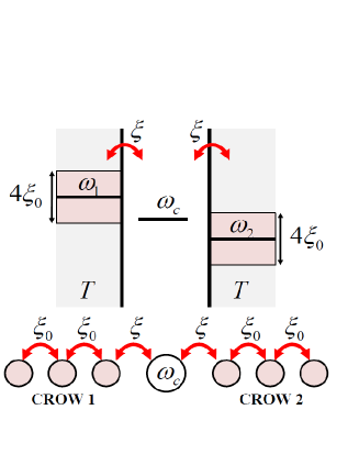
Figure 2: A nanocavity with frequency $\omega_{c}$ couple to two coupled resonator optical waveguides (CROWs).

V.2 Analytical solutions in the weak coupling regime

First, we shall discuss the cavity photonic dynamics. Consider the case where the nanocavity is initially empty: $\langle a(t_{0})\rangle=0$ and $n(t_{0})=0$. The cavity field and the cavity photon number at a later time, i.e. Eqs. (31) and (33), become

$$\langle a(t)\rangle=y(t)\ ,$$ (61a)

$$n(t)=\langle a^{{\dagger}}(t)a(t)\rangle=v(t,t)+|y(t)|^{2}\ .$$ (61b)

Here $y(t)$ is the driving-induced field given by Eq. (26b) and $v(t,t)$ is the photon correlation due to the thermal fluctuation in the waveguides, given by Eq. (26c). Only at zero temperature, we have $v(t,t)=0$. Then the cavity photon number equals to the absolute square of the cavity field, i.e. $n(t)=|\langle a(t)\rangle|^{2}$.

To see the dynamics of cavity field controlled through the driving field, we shall consider first the cavity decoupled to waveguides, i.e. $\xi_{1c}=\xi_{2c}=0$. In this situation, the photonic propagating function in the cavity is simply given by $u(t,t_{0})=e^{-i\omega_{c}(t-t_{0})}$ and the photon correlation function $v(t,t)=0$. Then, the cavity field and cavity photon number equal to $y(t)$ and $|y(t)|^{2}$, respectively, with

$$y(t)=\begin{cases}\frac{E_{0}}{\omega_{d}-\omega_{c}}[e^{-i\omega_{d}(t-t_{0})}-e^{-i\omega_{c}(t-t_{0})}]&\omega_{d}\neq\omega_{c}\\ &\\ E_{0}(t-t_{0})e^{-i(\omega_{c}(t-t_{0})+\frac{\pi}{2})}&\omega_{d}=\omega_{c}\end{cases}\ .$$ (62)

It shows that the cavity field is a coherent superposition of the cavity mode with the external driving field. If the driving field frequency differs from the cavity mode, the interference between the cavity mode and the driving field causing the photons jump in and out of the cavity with the Rabi frequency $(\omega_{d}-\omega_{c})/2$. When the driving field is in resonance with the cavity mode, the driving field would be completely absorbed into the cavity, and the cavity field amplitude increases linearly in time without an interference oscillation.

When the cavity couples to waveguides, generally it is not easy to find the analytical solution for $u(t,t_{0})$ and $v(t,t)$. One has to solve Eqs. (25b) and (26c) numerically to understand the photonic dynamics of the driven cavity. However, in the weak coupling regime, the memory effect is negligible so that the Born-Markov approximation can be applied Xio10012105 . Then the photonic propagating function and the correlation function in weak coupling limit can be approximated (see Appendix B) by

$$u(t,t_{0})\simeq e^{-(i\omega^{\prime}_{c}+\kappa)(t-t_{0})}\ ,$$ (63a)

$$v(t,t)\simeq\bar{n}(\omega^{\prime}_{c},T)[1-e^{-2\kappa(t-t_{0})}]\ ,$$ (63b)

where $\omega^{\prime}_{c}=\omega_{c}+\sum_{\alpha}\delta\omega_{\alpha}$ is a renormalized cavity frequency with frequency shift $\delta\omega_{\alpha}={\cal P}[\int\frac{d\omega}{2\pi}\frac{J_{\alpha}(\omega)}{\omega_{c}-\omega}]$. The damping rate $\kappa=\sum_{\alpha}\kappa_{\alpha}$ with $\kappa_{\alpha}=J_{\alpha}(\omega_{c})/2$ and the average photon number of the two waveguides $\bar{n}(\omega^{\prime}_{c},T)=\sum_{\alpha}J_{\alpha}(\omega^{\prime}_{c})n_{\alpha}(\omega^{\prime}_{c})/2\kappa$.

On the other hand, to solve the driving-induced field $y(t)$ in the BM limit, special care needs to be taken since the driving field has its own character frequency $\omega_{d}$ which is usually different from the cavity mode frequency $\omega_{c}$. Therefore, instead of applying directly the BM solution of Eq. (63a) into Eq. (26b), we have to use different character frequencies $\omega_{c}$ and $\omega_{d}$ for the homogeneous and inhomogeneous solutions of Eq. (25d) to find the BM limit of the driving-induced field $y(t)$. The detailed derivation is also given in Appendix B. The result is nontrivial:

$$y(t)\simeq\frac{E_{0}\exp{(-i\phi)}}{\sqrt{(\omega_{d}-\tilde{\omega}_{c})^{2}+\tilde{\kappa}^{2}}}[ e^{-i\omega_{d}(t-t_{0})}$$

$$-e^{-(i\omega^{\prime}_{c}+\kappa)(t-t_{0})}],$$ (64)

where $\phi=\tan^{-1}\frac{\tilde{\kappa}}{\omega_{d}-\tilde{\omega}_{c}}$, $\tilde{\omega}_{c}=\omega_{c}+\sum_{\alpha=1}^{2}\delta\tilde{\omega}_{\alpha}$ with the driving field induced frequency shift $\delta\tilde{\omega}_{\alpha}={\cal P}\int_{0}^{\infty}\frac{d\omega}{2\pi}\frac{J_{\alpha}(\omega)}{\omega_{d}-\omega}$. $\tilde{\kappa}=\sum_{\alpha=1}^{2}\tilde{\kappa}_{\alpha}$ with $\tilde{\kappa}_{\alpha}=J_{\alpha}(\omega_{d})/2$, located at the driving frequency rather than the cavity frequency. Correspondingly, the cavity field and the cavity photon number of Eq. (61) in the BM limit become

$$\langle a(t)\rangle \simeq\frac{E_{0}\exp{(-i\phi)}}{\sqrt{(\omega_{d}-\tilde{\omega}_{c})^{2}+\tilde{\kappa}^{2}}}[e^{-i\omega_{d}(t-t_{0})}$$

$$~{}~{}~{}~{}~{}~{}~{}~{}~{}~{}~{}~{}~{}~{}~{}~{}~{}~{}~{}~{}~{}~{}~{}~{}~{}-e^{-(i\omega^{\prime}_{c}+\kappa)(t-t_{0})}],$$ (65a)

$$n(t)\simeq ~{}\bar{n}(\omega^{\prime}_{c},T)[1-e^{-2\kappa(t-t_{0})}]$$

$$+\frac{E_{0}^{2}}{(\omega_{d}-\tilde{\omega}_{c})^{2}+\tilde{\kappa}^{2}}\big{[}1+e^{-2\kappa(t-t_{0})}$$

$$~{}~{}~{}~{}~{}-2e^{-\kappa(t-t_{0})}\cos{[(\omega_{d}-\omega^{\prime}_{c})(t-t_{0})]}\big{]}.$$ (65b)

As one see, the cavity field is a coherent superposition of the external driving field and the damped cavity mode, where the damping comes from the coupling of the cavity with waveguides that induces photon dissipation from the cavity into waveguides. This damping (dissipation) effect leads cavity mode to vanish in the steady limit. Only the driving field is remained in the cavity with a modified (amplified) field amplitude $E_{0}^{\prime}=\frac{E_{0}}{\sqrt{(\omega_{d}-\tilde{\omega}_{c})^{2}+\tilde{\kappa}^{2}}}$ and a phase shift $\phi$, as a feed-back effect from the coupling of the cavity with waveguides. The photon number in the cavity is then a combination of the driving-induced field plus a background noise from the thermal fluctuation of waveguides [$\sim\bar{n}(\omega^{\prime}_{c},T)$]. These analytical results help us to understand the driven cavity dynamics in the strong coupling regime. The corresponding numerical solution will be presented later.

Furthermore, the transport phenomena of photons flowing into the waveguides can be specified by the photocurrent which can be simplified as well in the weak coupling limit:

$$I_{\alpha}(t)= -2\kappa_{\alpha}\bar{n}(\omega^{\prime}_{c})e^{-2\kappa(t-t_{0})}$$

$$+\frac{2E_{0}^{2}\kappa_{\alpha}}{(\tilde{\omega}_{c}-\omega_{d})^{2}+\tilde{\kappa}^{2}}\Big{\{}\frac{\tilde{\kappa}_{\alpha}}{\kappa_{\alpha}}+e^{-2\kappa(t-t_{0})}$$

$$-(1+\frac{\tilde{\kappa}_{\alpha}}{\kappa_{\alpha}})e^{-\kappa(t-t_{0})}\cos{[(\omega_{d}-\omega^{\prime}_{c})(t-t_{0})]}$$

$$+\frac{\delta\omega_{\alpha}-\delta\tilde{\omega}_{\alpha}}{\kappa_{\alpha}}e^{-\kappa(t-t_{0})}\sin{[(\omega_{d}-\omega^{\prime}_{c})(t-t_{0})]}\Big{\}}.$$ (66)

The first term in Eq. (V.2) is the contribution of the waveguide thermal fluctuation, which would be vanish when the cavity is equilibrated with the waveguides. The remainders come from the response of the waveguides to the external driving field through the cavity, in which the first decay term is due to the dissipation of the cavity mode, the second and third decay terms are the thermal-fluctuation-induced decoherence (noise) of the cavity field. These three contributions together with the thermal-fluctuation-induced current (the first term) will vanish in the steady limit. The time-independent term in Eq. (V.2) is the steady photocurrent, which is determined by the cavity mode, the driving field frequency and the spectrum of the waveguide. When the driving field frequency lies outside the band of the waveguide $\alpha$, the steady photoncurrent vanishes because $\tilde{\kappa}_{\alpha}=J_{\alpha}(\omega_{d})/2=0$. On the other hand, the photocurrent flowing into the waveguide $\alpha$ becomes maximal when the driving field frequency lies at the band center of the waveguide $\alpha$, i.e. $\omega_{d}=\omega_{\alpha}$, see Eq. (60). This result shows that the nontrivial Born-Markovian solution in the presence of external driving field gives already a clear picture on the controllability of photonic transport in the photonic circuit through the external driving frequency.

V.3 Exact numerical solutions in both the weak and strong coupling regimes

Now, we turn to the exact numerical calculation for arbitrary coupling between the cavity and waveguides. We will focus on the situation where the frequency of the cavity lies between the band centers of the two waveguides, i.e. $\omega_{c}=(\omega_{1}+\omega_{2})/2$. In the numerical calculation, we take $\omega_{1}=9.5$GHz, $\omega_{2}=10.5$GHz, $\xi_{1}=\xi_{2}=\xi=0.3$GHz, $\xi_{1c}=\xi_{2c}=\xi_{c}$, and $E_{0}=10$GHz. We should first compare the above analytical BM solution in the weak coupling limit with the exact numerical solution of the cavity field amplitude, the cavity photon number and the photoncurrent, given by Eqs. (65) and (V.2) and Eqs. (61) and (43), respectively. The result is plotted in Fig. 3 where the coupling rate $\eta=\xi/\xi_{0}=0.5$ which belongs to a weak coupling and the BM approximation is applicable as we have shown in Wu1018407 . From Fig. 3, we see that in the weak coupling limit, the BM solution is in good agreement with the exact solution, in particular when the driving frequency $\omega_{d}=\omega_{1}$. When the driving frequency equals to the cavity mode frequency, the deviation between the exact solution and the BM solution becomes relatively large in the steady limit. This can be seen from Eq. (65) where the amplified cavity field amplitude in the BM limit, $E_{0}^{\prime}=\frac{E_{0}}{\sqrt{\delta\tilde{\omega}_{c}^{2}+\tilde{\kappa}^{2}}}$, becomes sensitive to the approximation. But the qualitative behavior of the BM solution is still in good agreement with the exact solution.

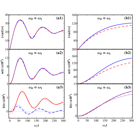
Figure 3: Comparison of the analytical solution in the weak coupling limit with the exact numerical solution at the coupling rate $\eta=\xi/\xi_{0}=0.5$ with different driving frequency. (a1)-(a1) and (a2)-(b2) are the cavity field amplitude and cavity photon number, respectively, with the BM solution (red dashed line) and the exact solution (blue solid line). (a3)-(b3) are the photocurrent $I_{1}(t)$ and $I_{2}(t)$ with the exact solution (red solid line and blue dashed line) and the BM solution (blue dotted line and red dotted-dashed line).

Next, we shall present the exact numerical solutions for different values of the coupling constants between the cavity and the waveguides, to examine the different photonic transport dynamics in the weak coupling as well as in the strong coupling regime. Fig. 4 shows the cavity field amplitude of Eq. (61) with different coupling strengths and different driving field frequencies. Fig. 4(a) and Fig. 4(b) correspond to the cases of the driving frequency being in resonance with the band center of CROW 1 and the cavity mode, respectively. Different curves in each plot correspond to different coupling strengths between the cavity and waveguides. In the weak coupling regime, the behavior of the cavity field amplitude highly depends on the driving field frequency. When the driving field is not in resonance to the cavity mode, the field amplitude oscillates (as a result of the superposition of the driving field with the cavity mode) and decay (due to the dissipation induced by the coupling of the cavity with waveguides). When the driving field is in resonance to the cavity mode ($\omega_{d}=\omega_{c}$), the field amplitude increases gradually without oscillation. These numerical results agree with the BM solution of Eq. (65a), as shown in Fig. 3. In the strong coupling regime, the field amplitude keep oscillating without decay in both cases. The absence of the damping (dissipation) is totally due to the non-Markovian memory effect, as we have pointed out recently Xio10012105 ; Wu1018407 . The complicated oscillating behavior (dotted red curve) in Fig. 4(a) is an interference effect between the driving field and the cavity mode with $\omega_{d}\neq\omega_{c}$. Only in the resonance case ($\omega_{d}=\omega_{c}$), the cavity field becomes coherent with the external driving field, as shown by the dotted red curve in Fig. 4(b).

Figure 4: The time evolution of the cavity field amplitude with different coupling strengthes: $\eta=0.5$ (solid green line), $1.0$ (dashed blue line) and $2.0$ (dotted red line). (a) The driving field frequency equals to the band center of the CROW 1. (b) The driving field frequency is in resonance to the cavity mode.

Fig. 5 shows the thermal fluctuation $v(t,t)$ and the average photon number $n(t)$ in the driven cavity for different coupling strengthes, different driving field frequencies and different initial temperatures. According to Eq. (61b), when the cavity is empty initially, the average cavity photon number is fully determined by the driving-induced field $|y(t)|^{2}$ and the thermal fluctuation induced correlation $v(t,t)$. As shown in Fig. 5, $v(t,t)$ almost equals to zero when $T=5$mK. In this case, $n(t)=|\langle a(t)\rangle|^{2}\simeq|y(t)|^{2}$, namely, the cavity field is a pure coherent field induced by the external driving field. When the temperature increases, the contribution of $v(t,t)$ is increased as well. At $T=5K$, the contribution from the thermal fluctuation is still very small in the weak coupling, in comparison with the contribution from the driving-induced field $y(t)$. However, $v(t,t)$ becomes comparable with $y(t)$ in the strong coupling, as shows in Fig. 5(a3)-(b3). With further increase of the temperature, thermal fluctuation would destroy the coherence of the cavity field if the driving field is weak.

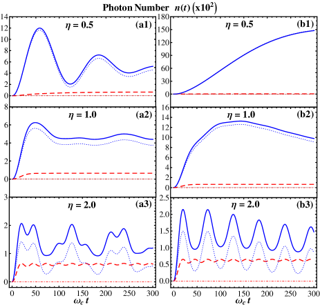
Figure 5: The time evolution of the thermal fluctuation $v(t,t)$ (red dashed and dotted-dashed curves) and the cavity intensity (blue solid and dotted curves) at different initial temperature ($T=5$K and $T=5$mK ) with different coupling strength. The left plots correspond to $\omega_{d}=\omega_{1}$ and the right plots for $\omega_{d}=\omega_{c}$.

Fig. 6 shows the photocurrents $I_{1}(t)$ and $I_{2}(t)$ flowing from the cavity into the CROWs in different driving frequencies and coupling strengthes. The frequency of the external driving field is the crucial factor for the control of the photocurrents. When the external driving field is in resonance to the cavity field, the photocurrents flowing through CROW 1 and CROW 2 are equal because of the symmetric configuration, as shown in Fig. 6(a2)-(c2). However, when the driving field is in resonance to the band center of CROW 1, the photocurrent $I_{1}(t)$ flowing through CROW 1 is dominated while the photocurrent $I_{2}(t)$ flowing through CROW 2 is suppressed, see Fig. 6(a1)-(c1). Similarly, when the driving field is in resonance to the band center of CROW 2, the photocurrent $I_{2}(t)$ becomes dominated and the photocurrent $I_{1}(t)$ is suppressed, as shown by Fig. 6(a3)-(c3). These results explicitly demonstrate the controllability of the photonic quantum transport through the driven cavity.

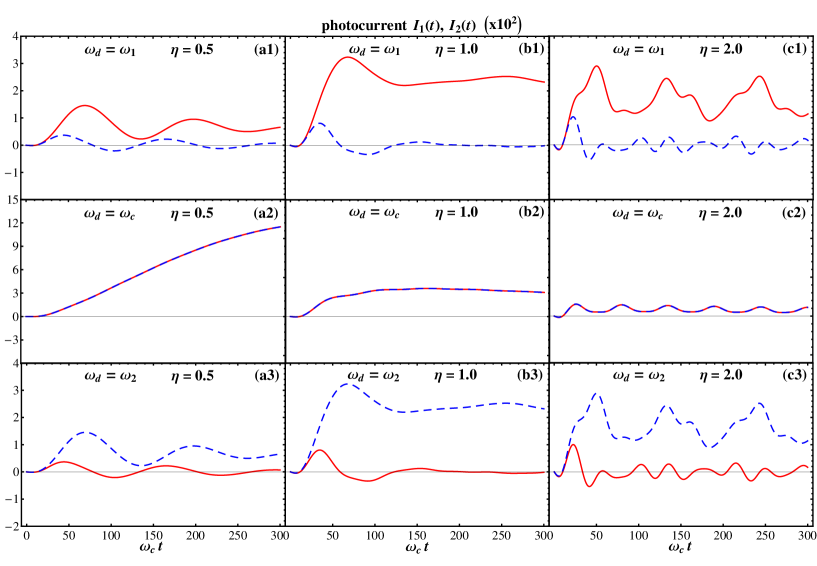
Figure 6: Photocurrent $I_{1}(t)$ (solid red line) and $I_{2}(t)$ (dashed blue line) in different coupling strength and driving frequencies. Here, the initial temperature $T=5$K.

The above numerical analysis show that the photonic dynamics and transport in an all-optical circuit can be manipulated efficiently through the external driving signals and the internal cavity-waveguide couplings. Photon dissipation and thermal fluctuation appear in all the cases. In the weak coupling limit, the cavity mode will decay so that only the driving-induced field plays the role in the photonic transport. The strong coupling between the cavity and the waveguides can largely suppress the cavity photon dissipation, due to the non-Markovian memory effect. In this case, the cavity mode can serve as a new control field in the photonic transport. The photonic thermal fluctuation can be suppressed by either lowing the temperature or making the device work in the high frequency region. These general properties provide a theoretical basis for the further development of integrated quantum photonic circuits.

VI SUMMARY AND PROSPECTIVE

In summary, we have established a quantum transport theory to describe photonic transport in photonic networks. The photonic networks consist of all-optical circuits incorporating photonic bandgap waveguides and driven resonators. The transient transport of photons in photonic networks is controlled through the driven resonators. The photonic dynamics of the driven resonators is determined by the master equation which is derived by treating the waveguides as an environment. The back-reactions between waveguides and resonators and thereby the dissipation and fluctuation arisen from the back-reactions are fully taken into account. The photocurrents flowing from the resonators into the waveguides that describe the photonic transport in the network are obtained directly from the master equation. The theory can be applied to photonic transport in photonic networks involving many photons as well as single photon.

Comparing with the electron transport in mesoscopic systems, we have shown several crucial differences for the photonic transport. Instead of the bias and gate voltage controls in electron transport, the photonic transport is manipulated through external driving fields applying to waveguides and resonators. Differing from the electron transport where the bias and gate voltages controls are imbedded into the spectral densities or the energy levels of the system, the external driving fields applying to waveguides and resonators turn out to be the modified driving fields acting explicitly on the resonators, as shown in the master equation of Eq. (III). The resulting lesser Green function, see Eq. (IV.2), and thereby the photocurrent, see Eq. (49), contain additional terms induced from the external driving fields that explicitly determine the photonic transport in the photonic network. In other words, the present theory shows that the transport controls through the external fields behave very differently for electrons and photons. Furthermore, the explicit initial state dependence also makes the present theory become more powerful in the study of transient transport phenomena.

As a simple illustration of the theory, we investigate the photonic transport dynamics of the driven nanocavity coupled to two waveguides. The cavity field, the cavity photon number as well as the photocurrents flowing through the waveguides are solved analytically in the weak coupling limit and are also exactly calculated numerically for strong couplings with different driving frequencies. Non-Markovian memory effects in the strong coupling regime are shown explicitly. The thermal fluctuation effect to the coherent property of the cavity field is also demonstrated. Moreover, the analytical and numerical results show the strong controllability of wavelength selective transport. The controllability together with the simplicity of the photonic circuit implementation in photonic crystals make it useful in the further development of integrated quantum photonic circuits.

We should further point out that the present theory can also be directly extended to investigate various photonic transport phenomena in other electromagnetic matematerials pcmeta and phonon transport in heat-conducting systems heatcond . The generality of the present theory incorporating with the Feynman-Vernon influence functional approach and the Keldysh’s nonequilibirum Green function technique together also makes it powerful in the investigation of open quantum system, in particular the nonequilibrium dynamics. The generalization of the present theory to the nonequilibirum dynamics of ultracold atomic Boson-Einstein condensation is in progress. Various novel devices, such as photon entanglement through photonic crystal waveguides Hug05 ; Tan11 , can be designed with the help of the present theory. And more applications will be presented in future works.

Appendix A Derivation of the propagating function

The influence functional of Eq. (III) modifies the original action of the system into an effective one, $e^{i(S_{S}[\boldsymbol{\alpha}^{*},\boldsymbol{\alpha}]-S_{S}[{\boldsymbol{\alpha}^{\prime}}^{*},\boldsymbol{\alpha}^{\prime}])}\mathscr{F}[\boldsymbol{\alpha}^{*}\boldsymbol{\alpha};{\boldsymbol{\alpha}^{\prime}}^{*}\boldsymbol{\alpha}^{\prime}]=e^{{i\over\hbar}S_{\rm eff}[\boldsymbol{\alpha}^{*}\boldsymbol{\alpha};{\boldsymbol{\alpha}^{\prime}}^{*}\boldsymbol{\alpha}^{\prime}]}$ which dramatically changes the dynamics of the driven resonators. The explicit change is manifested through the generating function of Eq. (III) by carrying out the path integral with respect to the effective action $S_{\rm eff}[\boldsymbol{\alpha}^{*}\boldsymbol{\alpha};{\boldsymbol{\alpha}^{\prime}}^{*}\boldsymbol{\alpha}^{\prime}]$. While the path integral $\mathcal{D}[\boldsymbol{\alpha}^{*}\boldsymbol{\alpha};{\boldsymbol{\alpha}^{\prime}}^{*}\boldsymbol{\alpha}^{\prime}]$ integrates over all the forward paths $\boldsymbol{\alpha}^{*}(\tau),\boldsymbol{\alpha}(\tau)$ and the backward paths ${\boldsymbol{\alpha}^{\prime}}^{*}(\tau),\boldsymbol{\alpha}^{\prime}(\tau)$ in the Bergman complex space bounded by $\boldsymbol{\alpha}^{*}(t)=\boldsymbol{\alpha}^{*}_{f},\boldsymbol{\alpha}(t_{0})=\boldsymbol{\alpha}_{0}$ and ${\boldsymbol{\alpha}^{\prime}}^{*}(t_{0})={\boldsymbol{\alpha}^{\prime}}^{*}_{0},\boldsymbol{\alpha}^{\prime}(t)=\boldsymbol{\alpha}^{\prime}_{f}$, respectively. Since $S_{\rm eff}[\boldsymbol{\alpha}^{*}\boldsymbol{\alpha};{\boldsymbol{\alpha}^{\prime}}^{*}\boldsymbol{\alpha}^{\prime}]$ is only a quadratic function in terms of the integral variables, the path integrals of Eq. (III) can be reduced to Gaussian integrals so that we can use the stationary path method to exactly carry them out Fey65 . The resulting propagating function is a function of the stationary paths:

$$\mathcal{J}(\boldsymbol{\alpha}_{f}^{*},\boldsymbol{\alpha}^{\prime}_{f},t|\boldsymbol{\alpha}_{i},{\boldsymbol{\alpha}^{\prime}}_{i}^{*},t_{0})=A(t)\exp\{\frac{1}{2}[\boldsymbol{\alpha}^{{\dagger}}_{f}\boldsymbol{\alpha}(t)+\boldsymbol{\alpha}^{{\dagger}}(t_{0})\boldsymbol{\alpha}_{i}$$

$$+{\boldsymbol{\alpha}^{\prime}}^{{\dagger}}(t)\boldsymbol{\alpha}^{\prime}_{f}+{\boldsymbol{\alpha}^{\prime}}^{{\dagger}}_{i}\boldsymbol{\alpha}^{\prime}(t_{0})]+\frac{i}{2}\int_{t_{0}}^{t}[({\boldsymbol{\alpha}^{\prime}}^{{\dagger}}(\tau)-\boldsymbol{\alpha}^{{\dagger}}(\tau))\boldsymbol{f}(\tau)$$

$$+\boldsymbol{f}^{{\dagger}}(\tau)(\boldsymbol{\alpha}^{\prime}(\tau)-\boldsymbol{\alpha}(\tau))]\}\ ,$$ (67)

where $A(t)$ is the contribution arisen from the fluctuations around the stationary paths and is given after Eq. (III). The stationary paths obey the equations of motion :

$$\frac{d\boldsymbol{\alpha}(\tau)}{d\tau} +i\boldsymbol{\omega}(\tau)\boldsymbol{\alpha}(\tau)+\int^{\tau}_{t_{0}}d\tau^{\prime}\mathbf{g}(\tau,\tau^{\prime})\boldsymbol{\alpha}(\tau^{\prime})$$

$$+ \int_{t_{0}}^{t}d\tau^{\prime}\widetilde{\mathbf{g}}(\tau,\tau^{\prime})[\boldsymbol{\alpha}(\tau^{\prime})-\boldsymbol{\alpha}^{\prime}(\tau^{\prime})]=-i\boldsymbol{f}(\tau),$$ (68a)

$$\frac{d\boldsymbol{\alpha}^{\prime}(\tau)}{d\tau} +i\boldsymbol{\omega}(\tau)\boldsymbol{\alpha}^{\prime}(\tau)$$

$$- \int_{\tau}^{t}d\tau^{\prime}\mathbf{g}(\tau,\tau^{\prime})\boldsymbol{\alpha}^{\prime}(\tau^{\prime})+\int_{t_{0}}^{t}d\tau^{\prime}\mathbf{g}(\tau,\tau^{\prime})\boldsymbol{\alpha}(\tau^{\prime})$$

$$+ \int_{t_{0}}^{t}d\tau^{\prime}\widetilde{\mathbf{g}}(\tau,\tau^{\prime})[\boldsymbol{\alpha}(\tau^{\prime})-\boldsymbol{\alpha}^{\prime}(\tau^{\prime})]=-i\boldsymbol{f}(\tau),$$ (68b)

subjected with the boundary conditions $\boldsymbol{\alpha}(t_{0})=\boldsymbol{\alpha}_{i}$ and $\boldsymbol{\alpha}^{\prime}(t)=\boldsymbol{\alpha}^{\prime}_{f}$. The equations of motion for $\boldsymbol{\alpha}^{{\dagger}}(\tau)$ and ${\boldsymbol{\alpha}^{\prime}}^{{\dagger}}(\tau)$ follow by exchanging $\boldsymbol{\alpha}$ and $\boldsymbol{\alpha}^{\prime}$ in Eq. (68) and taking a conjugate transpose, subjected to the boundary conditions ${\boldsymbol{\alpha}^{\prime}}^{{\dagger}}(t_{0})={\boldsymbol{\alpha}^{\prime}}^{{\dagger}}_{i}$ and $\boldsymbol{\alpha}^{{\dagger}}(t)=\boldsymbol{\alpha}^{{\dagger}}_{f}$.

To express the master equation independent of the coherent state representation, we shall further factorize the boundary values of the stationary paths, $\boldsymbol{\alpha}(t_{0})=\boldsymbol{\alpha}_{0}$, $\boldsymbol{\alpha}^{\prime}(t)=\boldsymbol{\alpha}^{\prime}_{f}$, through the following transformation:

$$\boldsymbol{\alpha}^{\prime}(\tau)-\boldsymbol{\alpha}(\tau)=\bar{\boldsymbol{u}}(\tau,t)(\boldsymbol{\alpha}^{\prime}_{f}-\boldsymbol{\alpha}(t)),$$ (69a)

$$\boldsymbol{\alpha}(\tau)=\boldsymbol{u}(\tau,t_{0})\boldsymbol{\alpha}_{0}+\boldsymbol{v}(\tau,t)(\boldsymbol{\alpha}^{\prime}_{f}-\boldsymbol{\alpha}(t))+\boldsymbol{y}(\tau)$$ (69b)

and a similar transformation for conjugate variables (with the exchange of $\boldsymbol{\alpha}$ with $\boldsymbol{\alpha}^{\prime}$ for the boundary values $\boldsymbol{\alpha}^{{\dagger}}(t)=\boldsymbol{\alpha}^{{\dagger}}_{f}$ and ${\boldsymbol{\alpha}^{\prime}}^{{\dagger}}(t_{0})={\boldsymbol{\alpha}^{\prime}}^{{\dagger}}_{0}$), where $\boldsymbol{u}(\tau,t_{0})$, $\bar{\boldsymbol{u}}(\tau,t)$, $\boldsymbol{v}(\tau,t)$ are $N$ by $N$ matrices, and $\boldsymbol{y}(\tau)$ is $1\times N$ matrix, $N$ is the dimension of the cavity system. Substituting the solutions of Eq. (69) into the equations of motion of Eq. (68) and comparing with the boundary values, we obtain the equations of motion for $\boldsymbol{u}(\tau,t_{0})$, $\bar{\mathbf{u}}(\tau,t)$, $\mathbf{v}(\tau,t)$ and $\boldsymbol{y}(\tau)$, given by Eq. (25). By multiplying $\bar{\boldsymbol{u}}^{{\dagger}}(\tau,t_{0})$ to Eq. (25a) and integrating $\tau$ from $t_{0}$ to $t$, we obtain the relation $\boldsymbol{u}(t,t_{0})=\bar{\boldsymbol{u}}^{{\dagger}}(t_{0},t)$. Similarly, we can also directly obtain the solutions of Eqs. (25) and (25d), which are given by Eq. (26).

Now, let $\tau=t_{0}$ in Eq. (69a) and $\tau=t$ in Eq. (69b), we can express $\boldsymbol{\alpha}(t)$ and $\boldsymbol{\alpha}^{\prime}(t_{0})$ in terms of the boundary conditions $\boldsymbol{\alpha}_{0}$ and $\boldsymbol{\alpha}^{\prime}_{f}$:

$$\boldsymbol{\alpha}(t)= \boldsymbol{w}(t)\big{[}\boldsymbol{u}(t,t_{0})\boldsymbol{\alpha}_{i}+\boldsymbol{v}(t,t)\boldsymbol{\alpha}^{\prime}_{f}+\boldsymbol{y}(t)\big{]}\ ,$$ (70a)

$$\boldsymbol{\alpha}^{\prime}(t_{0})= \boldsymbol{u}^{{\dagger}}(t,t_{0})[1-\boldsymbol{w}(t)\boldsymbol{v}(t,t)]\boldsymbol{\alpha}^{\prime}_{f}-\boldsymbol{u}^{{\dagger}}(t,t_{0})\boldsymbol{w}(t)\boldsymbol{y}(t)$$

$$+[1-\boldsymbol{u}^{{\dagger}}(t,t_{0})\boldsymbol{w}(t)\boldsymbol{u}(t,t_{0})]\boldsymbol{\alpha}_{0}\ ,$$ (70b)

here $\boldsymbol{w}(t)=[\boldsymbol{1}+\boldsymbol{v}(t,t)]^{-1}=\boldsymbol{w}^{{\dagger}}(t)$. Similarly, $\boldsymbol{\alpha}^{{\dagger}}(t_{0})$ and ${\boldsymbol{\alpha}^{\prime}}^{{\dagger}}(t)$ can be obtained by exchanging $\boldsymbol{\alpha}$ and $\boldsymbol{\alpha}^{\prime}$ in Eq. (70) and taking a conjugate transpose. Substituting these results with Eq. (69) into Eq. (67), we obtain the final form of the propagating function for the reduced density matrix given by Eq. (III).

Appendix B Analytical solution in weak coupling limit with external driving field

In this appendix, we shall present an analytical solutions in the weak coupling limit for the photonic network concerned in Sec. V. First, let us solve the photon propagating function $u(t,t_{0})$. To do so, let $u(t,t_{0})\equiv e^{-i\omega_{c}(t-t_{0})}A(t)$. Then Eq. (25a) is reduced to

$$\frac{dA(t)}{dt}+\int_{0}^{t-t_{0}}dt^{\prime}\mathbf{g}(t^{\prime})e^{i\omega_{c}t^{\prime}}A(t-t^{\prime})=0.$$ (71)

When the spectrum of the waveguides are broad enough and the coupling between the waveguides and the system is weak, the memory effect between the system and the reservoir can be ignored so that the Markov limit is reached. In other words, $A(t-\tau)$ in the integration can be replaced by $A(t)$ and the integration time $t^{\prime}$ can be considered much shorter in comparison with the character time $t$ of the cavity field An07042127 . Then,

$$\int_{0}^{t-t_{0}}dt^{\prime}\mathbf{g}(t^{\prime})e^{i\omega_{c}t^{\prime}}A(t-t^{\prime})$$

$$\simeq\Big{[}\lim_{t\rightarrow\infty}\int_{0}^{t-t_{0}}dt^{\prime}\mathbf{g}(t^{\prime})e^{i\omega_{c}t^{\prime}}\Big{]}A(t)=(i\delta\omega_{c}+\kappa)A(t),$$ (72)

where $\delta\omega_{c}=\sum_{\alpha=1}^{2}\delta\omega_{\alpha}$ is the cavity frequency shift with $\delta\omega_{\alpha}={\cal P}\int_{0}^{\infty}\frac{d\omega}{2\pi}\frac{J_{\alpha}(\omega)}{\omega_{c}-\omega}$. The cavity damping rate $\kappa=\sum_{\alpha=1}^{2}\kappa_{\alpha}$ with $\kappa_{\alpha}=J_{\alpha}(\omega_{c})/2$. Thus, the photonic propagating function is approximated analytically by

$$u(t,t_{0})\simeq e^{-(i\omega^{\prime}_{c}+\kappa)(t-t_{0})},$$ (73)

and the renormalized cavity frequency $\omega^{\prime}_{c}=\omega_{c}+\delta\omega_{c}$.

Next, we shall solve the correlation function $v(t,t)$ in the same approximation. Note that $\frac{v(t,t)}{dt}\neq\frac{v(\tau,t)}{d\tau}|_{\tau=t}$, one should not directly use Eq. (25) to solve $v(t,t)$. It is more convenient to take the time derivative of the solution $v(t,t)$ given by (26c) and utilize the Eq. (25a), which leads to

$$\frac{v(t,t)}{dt}+2{\rm Re}\int_{t_{0}}^{t}d\tau \mathbf{g}(t-\tau)v(\tau,t)$$

$$=2{\rm Re}{\int_{t_{0}}^{t}d\tau\tilde{\mathbf{g}}(t-\tau)\bar{u}(\tau,t)}.$$ (74)

Then using the same approximation of Eq. (72), we have

$${\rm Re}\int_{t_{0}}^{t}d\tau\mathbf{g}(t-\tau)v(\tau,t) \simeq{\rm Re}\int_{t_{0}}^{t}d\tau g(t-\tau)e^{i\omega_{c}(t-\tau)}v(t,t)$$

$$\simeq\kappa v(t,t),$$

$${\rm Re}\int_{t_{0}}^{t}d\tau\tilde{\mathbf{g}}(t-\tau)\bar{u}(\tau,t) \simeq{\rm Re}\int_{t_{0}}^{t}d\tau\tilde{g}(t-\tau)e^{i\omega^{\prime}_{c}(t-\tau)}$$

$$\simeq\sum_{\alpha=1}^{2}J_{\alpha}(\omega^{\prime}_{c})n_{\alpha}(\omega^{\prime}_{c}),$$ (75)

Thus, the solution of Eq. (74) is approximately given by

$$v(t,t)\simeq\bar{n}(\omega^{\prime}_{c},T)[1-e^{-2\kappa(t-t_{0})}],$$ (76)

where $\bar{n}(\omega^{\prime}_{c},T)=\sum_{\alpha=1}^{2}n_{\alpha}(\omega^{\prime}_{c})J_{\alpha}(\omega^{\prime}_{c})/2\kappa$. The analytical solutions of Eqs. (73) and (76) are the well-known Born-Markov limit of the cavity field coupled to a thermal bath.

With the external driving field $f(t)=E_{0}e^{-i\omega_{d}(t-t_{0})}$ being explicitly added, the equation of motion for the driving-induced field $y(\tau)$ becomes:

$$\frac{dy(t)}{dt}+i\omega_{c}y(t)+\int_{t_{0}}^{t}d\tau g(t-\tau)y(\tau)=-iE_{0}e^{-i\omega_{d}(t-t_{0})}.$$ (77)

The homogeneous solution of this equation is just $u(\tau,t_{0})$ with the character frequency $\omega_{c}$, whose BM limit solution has been given by Eq. (73). The inhomogeneous solution of $y(t)$ must have a form $Be^{-i\omega_{d}(t-t_{0})}$, where $B$ is a constant and $\omega_{d}$ is the character frequency. In the BM limit, using the same approximation but noting the different character frequency, we find that

$$B=\frac{E_{0}\exp{(-i\phi)}}{\sqrt{(\omega_{d}-\tilde{\omega}_{c})^{2}+\tilde{\kappa}^{2}}},$$ (78)

where $\phi=\tan^{-1}\frac{\kappa}{\omega_{d}-\tilde{\omega}_{c}}$, $\tilde{\omega}_{c}=\omega_{c}+\sum_{\alpha=1}^{2}\delta\tilde{\omega}_{\alpha}$ with the driving field induced frequency shift $\delta\tilde{\omega}_{\alpha}={\cal P}\int_{0}^{\infty}\frac{d\omega}{2\pi}\frac{J_{\alpha}(\omega)}{\omega_{d}-\omega}$ and $\tilde{\kappa}=\sum_{\alpha=1}^{2}\tilde{\kappa}_{\alpha}$ with $\tilde{\kappa}_{\alpha}=J_{\alpha}(\omega_{d})/2$. Put the homogeneous solution and the inhomogeneous solution together with the initial condition $y(t_{0})=0$, we obtain the driving-induced field in the BM limit:

$$y(t)\simeq\frac{E_{0}\exp{(-i\phi)}}{\sqrt{(\omega_{d}-\tilde{\omega}_{c})^{2}+\tilde{\kappa}^{2}}}\big{[}e^{-i\omega_{d}(t-t_{0})}-e^{-(i\omega^{\prime}_{c}+\kappa)(t-t_{0})}\big{]}.$$ (79)

From the above solution for the propagating function $u(\tau,t_{0})$, the correlation function $v(t,t)$ and the driving-induced field $y(t)$, it is easy to find analytically the cavity field and the cavity photon number in the BM limit, i.e. Eq. (65). Utilizing the similar approximation in the above derivation, the photocurrent flowing through the waveguide $\alpha=1,2$ in the BM limit are given by Eq. (V.2). Furthermore, we can also find the source term in Eq. (44) in the BM limit by substituting the BM solution of the cavity field, Eq. (65a), into Eq. (39a) :

$$S(t)= \frac{2\tilde{\kappa}E_{0}^{2}}{(\omega_{d}-\tilde{\omega}_{c})^{2}+\tilde{\kappa}^{2}}\Big{\{}1+e^{-\kappa(t-t_{0})}\cos{[(\omega_{d}-\omega^{\prime}_{c})(t-t_{0})]}$$

$$+\frac{\omega_{d}-\tilde{\omega}_{c}}{\tilde{\kappa}}e^{-\kappa(t-t_{0})}\sin{[(\omega_{d}-\omega^{\prime}_{c})(t-t_{0})]}\Big{\}}.$$ (80)

As a self-consistent check, the BM solutions of the cavity photon number, the driving source and the photocurrent flowing into waveguides satisfy the quantum continuous equation:

$$\frac{dn(t)}{dt}=S(t)-\sum_{\alpha=1}^{2}I_{\alpha}(t).$$ (81)

References

- (1) R. Ramaswami and K. N. Sivarajan, Optical Networks: A Practical Perspective (Morgan Kaufmann, San Francisco, CA, 1998).
- (2) J. D. Joannoupoulos, R. D. Meade, J. W. Winn, and R. D. Meade, Photonic Crystals: Modeling the Flow of Light (Princeton, New York, 2008).
- (3) M. Notomi, Rep. Prog. Phys. 73, 096501 (2010).
- (4) S. Noda, A. Chutinan, and M. Imada, Nature 407, 608 (2000); Y. Akahane, T. Asano, B. S. Song, and S. Noda, Nature, 425, 944 (2003).
- (5) A. Yariv, Y. Xu, R. K. Lee, and A. Scherer, Opt. Lett. 24, 711 (1999); M. Bayindir, B. Temelkuran, and E. Ozbay, Phys. Rev. Lett. 84, 2140 (2000).
- (6) H. Gersen, T. J. Karle, R. J. P. Engelen, W. Bogaerts, J. P. Korterik, N. F. van Hulst, T. F. Krauss, and L. Kuipers1, Phys. Rev. Lett. 94, 073903 (2005); T. Baba, Nature Photon. 2, 465 (2008); R. M. De La Rue, Nat. Photon. 2, 715 (2008).
- (7) K. Nozaki, T. Tanabe, A. Shinya, S. Matsuo, T. Sato, H. Taniyama, and M. Notomi, Nat. Photon. 4, 477 (2010).
- (8) S. H. Fan, P. R. Villeneuve, J. D. Joannopoulos, Opt. Express 3, 4 (1998); H. G. Park, C. J. Barrelet, Y. Wu, B. Ting, F. Qian and C. M. Lieber, Nat. Photon. 2, 622 (2008).
- (9) T. Baba, Nature Photon. 1, 11 (2007); Q. Xu, P. Dong, and M. Lipson, Nat. Phys. 3, 406 (2007).
- (10) V. S. C. Manga Rao and S. Hughes, Phys. Rev. Lett. 99, 193901 (2007).
- (11) W. Yuan, L. Wei, T. T. Alkeskjold, A. Bjarklev, and O. Bang, Opt. Express 17, 19356 (2009); D. J. J. Hua, P. Shum, C. Lu, X. W. Sun, G. B. Ren, X. Yu and G. H. Wang, Opt. Commun. 282, 2343 (2009).
- (12) F. Du, Y. Q. Lu, and S. T. Wu, Appl. Phys. Lett. 85, 2181 (2004); N. Malkova and C. Z. Ning, J. Opt. Soc. Am. B 23, 978 (2006).
- (13) D. Psaltis, S. R. Quake, and C. Yang, Nature 442, 381 (2006); C. Monat, P. Domachuk, and B. J. Eggleton, Nat. Photon. 1, 106 (2007); L. Scolari, S. Gauza, H. Xianyu, L. Zhai, L. Eskildsen, T. T. Alkeskjold, S. T. Wu, and A. Bjarklev, Opt. Express 17, 3754 (2009).
- (14) W. Park, and J. B. Lee, Appl. Phys. Lett. 85, 4845(2004).
- (15) Y. Kanamori, K. Takahashi, and K. Hane, Appl. Phys. Lett. 95, 171911 (2009); X. Y. Chew, G. Y. Zhou, F. S. Chau, J. Deng, X. S. Tang, and Y. C. Loke, Opt. Lett. 35, 2517 (2010).
- (16) P. Lambropoulos, G. Nikolopoulos, T. R. Nielsen and S. Bay, Rep. Prog. Phys. 63, 455 (2000).
- (17) D. Mogilevtsev and S. Kilin, Theoretical Tools for Quantum Optics in Structured Media Progress in Optics, 54, 89-148 (2010).
- (18) E. Yablonovitch, Phys. Rev. Lett. 58, 2059 (1987); S. John, Phys. Rev. Lett. 58, 2486 (1987).
- (19) S. John and J. Wang, Phys. Rev. Lett. 64, 2418 (1990); Phys. Rev. B 43, 12 772 (1991); S. John and T. Quang, Phys. Rev. A 50, 1764 (1994).
- (20) S. Kilin and D. Mogilevtsev, Laser Phys. 2 153 (1992).
- (21) A. G. Kofman, G. Kurizki, and B. Sherman, J. Mod. Opt. 41, 353 (1994).
- (22) T. Quang, M. Woldeyohannes, S. John, and G. S. Agarwal, Phys. Rev. Lett. 79, 5238 (1997); S. John and T. Quang, Phys. Rev. Lett. 78, 1888 (1997); M. Florescu and S. John, Phys. Rev. A 64, 033801 (2001).
- (23) H. N. Xiong, W. M. Zhang, X. Wang and M. H. Wu, Phys. Rev. A 82, 012105 (2010).
- (24) M. H. Wu, C. U Lei, W. M. Zhang and H. N. Xiong, Opt. Express 18, 18407 (2010).
- (25) J. Schwinger, J. Math. Phys. 2, 407 (1961); L. V. Keldysh, Sov. Phys. JETP, 20, 1018 (1965).
- (26) L. P. Kadanoff, G. Baym, Quantum Statistical Mechanics, (Benjamin, New York, 1962)
- (27) R. P. Feynman and F. L. Vernon, Ann. Phys. 24, 118 (1963).
- (28) K. C. Chou, Z. B. Su, B. L. Hao, and L. Yu, Phys. Rep. 118, 1 (1985).
- (29) J. Rammer and H. Smith, Rev. Mod. Phys. 58, 323 (1986).
- (30) W. M. Zhang and L. Wilets, Phys. Rev. C 45, 1900 (1992).
- (31) H. Haug and A. P. Jauho, Quantum Kinetics in Transport and Optics of Semiconductors, Springer Series in Solid-State Sciences 123, 2nd Ed. (Springer-Verlag, Berlin, 2008),
- (32) A. J. Leggett, S. Chakravarty, A. T. Dorsey, M.P. Fisher, A. Garg, and W. Zwerger, Rev. Mod. Phys. 59, 1 (1987).
- (33) W. H. Zurek, Phys. Today 44 (10), 36 (1991); Rev. Mod. Phys. 75, 715 (2003).
- (34) A. O. Caldeira and A. J. Leggett, Physica A 121, 587 (1983).
- (35) B. L. Hu, J. P. Paz, and Y. H. Zhang, Phys. Rev. D 45, 2843 (1992).
- (36) H.-P. Breuer and F. Petruccione, The Theory of Open Quantum Systems, (Oxford University Press, Oxford, 2002).
- (37) U. Weiss, Quantum Dissipative Systems, (3rd Ed. World Scientific, Singapore, 2008).
- (38) E. Calzetta and B. L. Hu, Nonequilibrium Quantum Field Theory, (Cambridge University Press, New York, 2008).
- (39) H. Schoeller and G. Schön, Phys. Rev. B 50, 18436 (1994).
- (40) J. S. Jin, X. Zheng, and Y. J. Yan, J. Chem. Phys. 128, 234703 (2008).
- (41) J. S. Jin, M. W. Y. Tu, W. M. Zhang and Y. J. Yan, New J. Phys 12, 083013 (2010).
- (42) M. W. Y. Tu and W. M. Zhang, Phys. Rev. B 78, 235311 (2008).
- (43) M. W. Y. Tu, M. T. Lee and W. M. Zhang, Quantum Inf. Process, 8, 631, (2009).
- (44) C. Viviescas and G. Hackenbroich, Phys. Rev. A 67, 013805 (2003).
- (45) R. J. Glaber and M. Lewenstein, Phys. Rev. A 43, 467 (1991).
- (46) H. Feshbach, Ann. Phys. 19, 287-313 (1962).
- (47) J. H. An, and W. M. Zhang, Phys. Rev. A 76, 042127 (2007); J. H. An, M. Feng, and W. M. Zhang, Quantum Inf. Comput. 9, 0317 (2009).
- (48) H. J. Carmichael, An Open Systems Approach to Quantum Optics, Lecture Notes in Physics, Vol. m18 (Springer-Verlag, Berlin, 1993).
- (49) W. M. Zhang, D. H. Feng and R. Gilmore, Rev. Mod. Phys. 62, 867 (1990).
- (50) R. Karrlein and H. Grabert, Phys. Rev. E 55, 153 (1997).
- (51) F. Haake, and R. Reibold, Phys. Rev. A 32, 2462 (1985).
- (52) J. J. Halliwell and T. Yu, Phys. Rev. D 53, 2012 (1996).
- (53) G. W. Ford and R. F. O Connell, Phys. Rev. D 64, 105020 (2001).
- (54) T. Strunz and T. Yu, Phys. Rev. A 69, 052115 (2004).
- (55) C.-H. Chou, T. Yu, and B. L. Hu, Phys. Rev. E 77, 011112 (2008).
- (56) J. P. Paz and A. J. Roncaglia, Phys. Rev. Lett. 100, 220401 (2008); Phys. Rev. A 79, 032102 (2009).
- (57) H.-P. Breuer, B. Kappler, and F. Petruccione, Phys. Rev. A, 59 1633 (1999).
- (58) Q.-J. Tong, J.-H. An, H.-G. Luo, C. H. Oh, Phys. Rev. A 81, 052330 (2010).
- (59) Y. Liu, Z. Wang, M. H. Han, S. H. Fan, and R. Dutton, Opt. Express, 13, 4539 (2005).
- (60) M. Engheta, Science 317, 1698 (2007).
- (61) L. Wang and B. Li, Phys. World 21, 27 (2008); C. R. Otey, W. T. Lau, and S. H. Fan, Phys. Rev. Lett. 104, 154301 (2010).
- (62) S. Hughes, Phys. Rev. Lett. 94, 227402 (2005); ibid. 98, 083606 (2007).
- (63) H. T. Tan and W. M. Zhang, in preparation (2011).
- (64) Usually the stationary path (or stationary phase) method is an approximation to path integral calculations. When the path integrals can be reduced to Gaussian integrals, the stationary path method will lead to an exact solution. For more detailed discussion, see R. P. Feynman and A. R. Hibbs, Quantum Mechanics and Path Integrals (McGraw-Hill, 1965).