Can a traveling wave connect two unstable states?
The case of the nonlocal Fisher equation
Abstract
This note investigates the properties of the traveling waves solutions of the nonlocal Fisher equation. The existence of such solutions has been proved recently in [2] but their asymptotic behavior was still unclear. We use here a new numerical approximation of these traveling waves which shows that some traveling waves connect the two homogeneous steady states and , which is a striking fact since is dynamically unstable and is unstable in the sense of Turing.
Key-words Nonlocal Fisher equation, Turing instability, traveling waves.
AMS Subject Classification: 35B36, 92B05, 37M99.
1 Introduction
For the semilinear equation
| (1) |
a traveling wave can connect the two steady states and in various situations. This is the case when is unstable and is stable (Fisher/monostable). This is also the case when and are both stable (Allen-Cahn/bistable). It is known that these waves are attractive and are obtained as the long time limit of the dynamics (1) associated with compactly supported initial data (see [6]). When and are unstable, in between there is a stable steady state of which prevents any traveling wave to exists.
For systems and non-local equations, the classification becomes more complicated because a steady state can be Turing unstable, which means that is unstable with respect to some periodic perturbations in a bounded range of periods. In this note we consider the nonlocal Fisher equation (2), the simplest to produce Turing instability.
| (2) |
with
| (3) |
The steady state can be Turing unstable when the Fourier transform of changes sign and is large enough (see [3, 4, 2]). This creates several differences with the monostable or bistable equations.
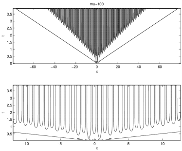
First of all, one can observe that the solution of (2) associated with a compactly supported initial datum does not converge, for large times, toward the traveling wave but it converges towards a more complicated structure (see [3], [4] and [5]). The numerical simulation presented in b) of Figure 4 shows that the solution of the evolution equation converges to a pulsating front, that is a function which is periodic in its second variable. These types of fronts typically arise in the framework of reaction-diffusion equations with periodic coefficients ([1], [7]). In a) of Figure 4, the solution seems to converge to the superposition of a traveling wave and a pulsating front, with two different speeds. These periodic patterns are a symptom of Turing instability on the full line .
a)
 b)
b)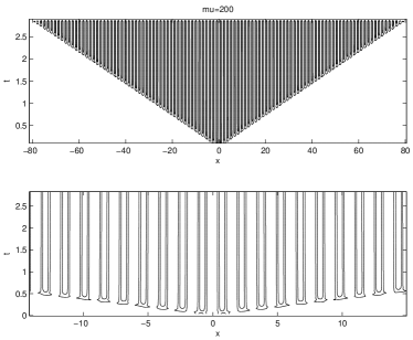
Secondly, it is proved in [2] that a traveling wave always exists for all , with a generalized formulation
| (4) |
The authors were only able to obtain, due to the nonlocal effect, the weak boundary condition at rather than the expected condition . When is small enough or when the Fourier transform of the kernel is positive everywhere, the traveling wave connects to . But this leaves open the question to know whether for large, the traveling wave solution of (5) connects the (dynamically) unstable state to a stable periodic state or to the Turing unstable state . Also, when can take negative values, it is proved in [2] that for large enough monotonic traveling waves cannot exist.
In the sequel, we will firstly focus on the case and
| (5) |
Then we also test two other cases
| (6a) | |||
| (6b) |
In all these cases, takes negative values. For instance, for (5), . Finally, to complete the tests, the traveling waves for the Gaussian kernel
| (7) |
which has positive Fourier transform, are displayed.
2 The algorithm
Numerically one can only solve the problem on a bounded domain of length (this is also the analytical construction in [2])
| (8) |
The convolution is computed by extending by 1 on and on . The parameter , small enough, is needed for technical reasons but intuitively its value has to be below the oscillations observed in Figure 2.
Our algorithm for solving (8) is to divide the computational domain into two parts: and . Being given , in each interval an elliptic equation with Dirichlet boundary conditions is solved
| (9) |
The convolution term is computed by defining as on , and , on and on .
But the equation does not necessarily hold true at . We define so as to impose that the jump of derivatives at zero vanishes
| (10) |
We can write abstractly this problem as a fixed point for a system of two equations . It is straightforward to make it discrete using finite differences. The most efficient way to solve it is to use Newton iterations.
3 The numerical results
3.1 Convergence of the scheme
The numerical results we present in this section are obtained with the hat function in (5), and we study the effect of the bifurcation parameter . The diffusion term is treated implicitly by centered three point finite difference while the reaction term is put explicit.
In order to verify that the iterative scheme described in section 2 converges to the right solution, a crucial quantity to look at is the truncation errors at zero
Here are the values of at the grid points . The convergence results are displayed in Table 1. One can see that converges to zero as , which shows that our numerical results is a good approximation of (8) on the whole computational domain. Note that better accuracy of can be obtained if we use higher order numerical integration methods for the convolution term.
| 20 | 0.04 | 3.0619 | 15.3670 | 40 | 0.04 | 15.3670 | 80 | 0.04 | 15.3670 | ||
| 20 | 1.7883 | 15.4930 | 40 | 0.02 | 15.5028 | 80 | 0.02 | 15.4930 | |||
| 20 | 0.9721 | 15.5368 | 40 | 0.01 | 15.5319 | 80 | 0.01 | 15.5319 | |||
| 20 | 0.5075 | 15.5429 | 40 | 0.005 | 15.5429 | 80 | 0.005 | 15.5429 |
3.2 Convergence of the traveling waves to
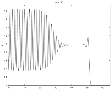
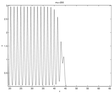
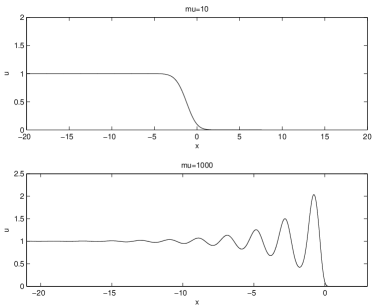
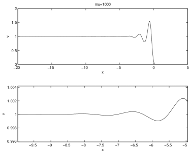
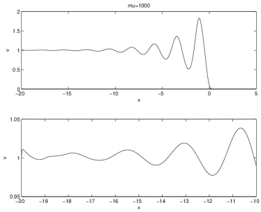
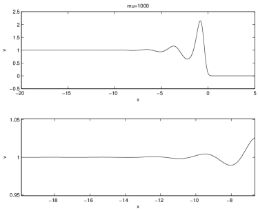
The traveling wave shapes for , and for kernel (5) are depicted in Figure 2. When , we observe a monotone traveling wave which connects to , as for the local Fisher equation. When grows, some oscillations appear. Numerically, when we increase , the amplitudes of the tail decrease and the bigger is, the slower the amplitudes decrease. The shapes of suggest that though is Turing unstable with the kernel (5) when and , the traveling waves will still connect to .
We do not obtain the same type of structure than when we compute the solution of the evolution equation depicted in Figure 4. This means that there exist some traveling waves that connect to , but that these waves do not attract the solution of the Cauchy problem associated with compactly supported initial data.

3.3 Monotonicity of the traveling waves
Lastly, we consider the critical value of for which the monotonicity of the traveling waves is broken. Since the monotone traveling waves always connect to , we perform the linearization, close to , by assuming with a real positive number 111We do not know if such a linearization is legitimate, but the technical arguments used in [2] to prove non-monotonicity for large are close to a linearization. After inserting this form into (4), using and the smallness of , can be determined by through the equation
| (11) |
a quadratic equation for , which gives . Thus the critical that makes no longer exist is .
We have checked that this threshold is correct on the numerical values. The maximum of is when , but exceeds slightly when . In Figure 2 with , the wave is nearly monotonic, but, checking the numerical values, the maximum of is . This indicates that actually might be not monotone even for finite.
In [2] the authors have proved that, when , the traveling wave is not monotone. One open question is to know if the traveling wave is monotone when . Our simulation answers positively to this open question numerically.
3.4 Traveling wave shapes for kernels in (6)
The numerical results with kernels in (6) are depicted in Figure 3. With large , we can see similar phenomena such that some oscillations appear and the waves become nonmonotone. For the two kernels in (6), the state is Turing unstable as for (6) and Figure 3 suggests again that the traveling waves will connect to .
Finally, to complete the tests, we show the traveling wave for the Gaussian kernel (7) for in Figure 4.
References
- [1] H. Berestycki, F. Hamel, Front propagation in periodic excitable media, Comm. Pure Appl. Math. 55, 949–1032, 2002.
- [2] H. Berestycki, G. Nadin, B. Perthame and L. Ryzhik, The non-local Fisher-Kpp equation: traveling waves and steady states. Nonlinearity (22), 2813–2844, 2009.
- [3] M. A. Fuentes, M. N. Kuperman and V. M. Kenkre, Nonlocal interaction effects on pattern formation in population dynamics, Phys. Rev. Lett. 91(15), 15810414.1–15810414.4, 2003.
- [4] S. Genieys, V. Volpert and P. Auger, Pattern and waves for a model in population dynamics with nonlocal consumption of resources, Math. Modelling Nat. Phenom. 1, 65–82, 2006.
- [5] S. A. Gourley, Travelling front solutions of a nonlocal Fisher equation, J. Math. Biol. 41(3), 2000.
- [6] A.N. Kolmogorov, I.G. Petrovsky and N.S. Piskunov, Etude de l équation de la diffusion avec croissance de la quantité de matière et son application à un problème biologique, Bulletin Université d’Etat à Moscou (Bjul. Moskowskogo Gos. Univ.), 1–26, 1937.
- [7] N. Shigesada, K. Kawasaki, E. Teramoto, Traveling periodic waves in heterogeneous environments, Theor. Population Biol. 30, 143–160, 1986.