M-theory and Seven-Dimensional Inhomogeneous Sasaki-Einstein Manifolds

Abstract

Seven-dimensional inhomogeneous Sasaki-Einstein manifolds $Y^{p,k}(KE_{4})$ present a challenging example of AdS/CFT correspondence. At present, their field theory duals for $KE_{4}=\mathbb{CP}^{2}$ base are proposed only within a restricted range $3p/2\leq k\leq 2p$ as ${\cal N}=2$ quiver Chern-Simons-matter theories with $SU(N)\times SU(N)\times SU(N)$ gauge group, nine bifundamental chiral multiplets interacting through a cubic superpotential. To further elucidate this correspondence, we use particle approximation both at classical and quantum level. We setup a concrete AdS/CFT mapping of conserved quantities using geodesic motions, and turn to solutions of scalar Laplace equation in $Y^{p,k}$. The eigenmodes also provide an interesting subset of Kaluza-Klein spectrum for $D=11$ supergravity in ${\rm AdS}_{4}\times Y^{p,k}$, and are dual to protected operators written in terms of matter multiplets in the dual conformal field theory.

1 Introduction

Thanks to the recent proposals in terms of Chern-Simons-matter theories Bagger:2007jr ; Aharony:2008ug , we now have a number of concrete examples for ${\rm AdS}_{4}/{\rm CFT}_{3}$. On the gravity side the internal space of M-theory is usually given as a toric Sasaki-Einstein seven-manifold, while on the other side of the duality we have a $D=3,\,{\cal N}=2$ theory whose gauge symmetry and interactions are summarised by a quiver diagram. For the case of Aharony-Bergman-Jafferis-Maldacena (ABJM) model Aharony:2008ug M2-branes are put on an orbifold $\mathbb{C}^{4}/\mathbb{Z}_{k}$, where $k$ is the inverse coupling constant. For other orbifolds of $\mathbb{C}^{4}$ whose gauge dual can be derived using D-brane intersection models, see e.g. Imamura:2008nn .

Except for the ${\cal N}=6$ model Aharony:2008ug which is in principle amenable to exact computations in both string theory and the gauge field theory, most of other ${\rm AdS}_{4}/{\rm CFT}_{3}$ examples are less well-understood. Usually they are justified only by the calculation of the vacuum moduli space for the given quiver Chern-Simons theory, and the fact that it agrees with the toric data of the eight-dimensional transverse space where the M2-branes are allowed to move. Many such duality “examples” can be found for instance in Martelli:2008si ; Hanany:2008cd ; Ueda:2008hx ; Franco:2009sp ; Martelli:2009ga ; Benini:2009qs .

For improvement one can use classical membranes as a probe. Rotating membrane solutions in the large energy limit can provide nontrivial quantitative predictions for long operators in the dual field theory. This program was initiated by the seminal paper Gubser:2002tv , and shown to give a starting point for semi-classical quantization of string theory in ${\rm AdS}_{5}\times S^{5}$ Tseytlin:2004xa . Nontrivial classical membrane solutions in ${\rm AdS}_{4}\times S^{7}$ which are studied in the context of Chern-Simons duals can be found e.g. Bozhilov:2007bi ; Ahn:2008gd ; Bozhilov:2007wn .

More intricate backgrounds for ${\rm AdS}_{4}/{\rm CFT}_{3}$ are given by $d=7$ Sasaki-Einstein (SE) manifolds. SE manifolds are odd-dimensional and their metric cone provides a singular Calabi-Yau space. There are several examples of seven-dimensional SE manifolds which can be constructed as a coset. For instance the explicit metrics of so-called $Q^{1,1,1},M^{1,1,1},V^{5,2}$ manifolds have been known for many years. Mainly as a potential model-building tool for particle physics, the Kaluza-Klein reduction spectra for backgrounds ${\rm AdS}_{4}\times{\cal M}_{7}$, with for instance ${\cal M}_{7}=S^{7},Q^{1,1,1},M^{1,1,1}$ were studied extensively in the past Pope:1984ig ; Duff:1986hr . Of course in AdS/CFT such supergravity modes correspond to supersymmetric operators whose conformal dimensions are protected from quantum corrections. Anomalous dimensions of many non-BPS operators can be computed using classical membrane solutions moving in ${\rm AdS}_{4}\times{\cal M}_{7}$. Membranes rotating in toric SE spaces $Q^{1,1,1},M^{1,1,1}$, and also in non-toric $V^{5,2}$ have been studied and their implications on dual CFT operaors have been reported Kim:2010ck ; Lee:2010hjb ; q111 . Ideally one would like to compare such supergravity side results with genuine field theory computations. But the dual theories are all strongly-coupled and at present it is very difficult to extract any quantitative data except for the spectrum of supersymmetric operators.

Then it is logically the next step to turn to inhomogeneous SE manifolds. Five-dimensional SE manifolds other than $T^{1,1}=SU(2)\times SU(2)/U(1)$ are first constructed explicitly in Gauntlett:2004yd . Dubbed $Y^{p,q}$, they are topologically $S^{2}\times S^{3}$ and equipped in general with a cohomogeneity-1 metric and include $T^{1,1}$ as a special case. They are also toric and have isometry $SU(2)\times U(1)\times U(1)$, and the dual quiver gauge theories are identified in Martelli:2004wu . It constituted a highly nontrivial check of AdS/CFT correspondence that the volume of $Y^{p,q}$ match exactly with the purely field-theoretical computation of central charges using $a$-maximization Intriligator:2003jj ; Martelli:2005tp . For more works on the duality involving $Y^{p,q}$ spaces, see e.g. Bertolini:2004xf ; Benvenuti:2004dy ; Berenstein:2005xa ; Franco:2005zu ; Bertolini:2005di ; Caceres:2010ju .

The construction of cohomogeneity-1 SE manifolds can be generalized to arbitrary higher dimensions Gauntlett:2004hh . Given a $2n$-dimensional regular Kähler-Einstein manifold, roughly speaking one can add a squashed $S^{3}$ fibration, give a SE metric to the entire $2n+3$-dimensional space, and make it globally regular at the same time. In this paper we are interested in M-theory backgrounds ${\rm AdS}_{4}\times{\cal M}_{7}$ where ${\cal M}_{7}=Y^{p,k}(\mathbb{CP}^{2})$ or $Y^{p,k}(\mathbb{CP}^{1}\times\mathbb{CP}^{1})$. Here $p,k\in\mathbb{Z}$ determine the toric data and for special cases $Y^{1,1}(\mathbb{CP}^{1}\times\mathbb{CP}^{1})=Q^{1,1,1},Y^{2,3}(\mathbb{CP}^{2})=M^{1,1,1}$ Martelli:2008rt . Gauge theory duals for ${\rm AdS}_{4}\times Y^{p,k}(\mathbb{CP}^{2})$ have been proposed and their vacuum moduli space in the mesonic branch is shown to match the (metric cone of) SE space for some specific range of $p,k$ Martelli:2008si .

In this paper we take a modest start in the study of conjecture for ${\rm AdS}_{4}\times Y^{p,k}$. We analyze some geodesic motions and also solve the scalar Laplace equation in $Y^{p,k}(\mathbb{CP}^{1}\times\mathbb{CP}^{1})$ and $Y^{p,k}(\mathbb{CP}^{2})$. Note that for $d=5$ the geodesics and their AdS/CFT interpretation was given in Benvenuti:2005cz , and the scalar Laplace equation in $Y^{p,q}$ was studied in Kihara:2005nt , whose steps we will closely follow in Sec.4. We will establish the mapping between the particle solutions and CFT operators, and also elucidate their conserved charges. The solutions of Laplace equation in $Y^{p,k}$ also provide an interesting subset of Kaluza-Klein spectrum. We present some of the simplest nontrivial solutions explicitly, and argue they are dual to the shortest chiral primary operators written purely in terms of scalar fields.

This paper is organized as follows. In Sec.2 we give a short introduction to $Y^{p,k}$, mainly to fix the notation and provide essential information. In Sec.3 we consider particle orbiting in SE space and establish a dictionary between supergravity description and the quiver Chern-Simons theory. Sec.4 is the main part where we study the Laplace equation and present some of the lowest lying modes explicitly. We conclude in Sec.5.

2 Sasaki-Einstein Seven-Manifolds $Y^{p,k}$

In this paper we are interested in the aspects of ${\rm AdS}_{4}/{\rm CFT}_{3}$ correspondence for M-theory. The eleven-dimensional metric can be written as a direct product of a four-dimensional anti-de Sitter space and a seven-dimensional compact manifold which is Einstein,

$$ds^{2}_{11}=L^{2}(\frac{1}{4}ds^{2}_{4}+ds^{2}_{7}).$$ (1)

Both the four and seven dimensional part (with metrics $ds^{2}_{4}$ and $ds^{2}_{7}$) have unit radius and satisfy

$$Ric_{4}=-3g_{4},\quad Ric_{7}=6g_{7}.$$ (2)

The Einstein equation is satisfied with the inclusion of a non-vanishing four-form field $G^{(4)}=\frac{3L^{3}}{8}{\rm Vol}_{4}$. It is well-known that when $X^{7}$ is Sasakian as well as Einstein, or if its metric cone provides a locally Calabi-Yau space, the overall M-theory background is supersymmetric with eight supercharges. The simplest such examples are $Q^{1,1,1}$ and $M^{1,1,1}$. These manifolds are toric, homogeneous, and can be considered as natural generalizations of the (base of) conifold $T^{1,1}$ to seven dimensions. The Kaluza-Klein reduction spectra can be found in ref.Pope:1984ig . Their dual CFTs as supersymmetric Chern-Simons matter theory are proposed in refs. Franco:2009sp ; Martelli:2008si ; Hanany:2008cd . Classical solutions of rotating membranes in those backgrounds are constructed for instance in Kim:2010ck ; q111 . $Q^{1,1,1}$ and $M^{1,1,1}$ can be also treated as special limiting cases of the generically inhomogeneous $Y^{p,k}$ manifolds which are our main interest in this paper. For completeness let us record their metrics here. $Q^{1,1,1}$ is a twisted $U(1)$ fibration over $\mathbb{CP}^{1}\times\mathbb{CP}^{1}\times\mathbb{CP}^{1}$ with

$$ds_{7}^{2}=\frac{1}{16}(d\psi+\sum_{i=1}^{3}\cos\theta_{i}d\phi_{i})^{2}+\frac{1}{8}\sum_{i=1}^{3}(d\theta_{i}^{2}+\sin^{2}\theta_{i}d\phi_{i}^{2})\,,$$ (3)

and satisfies $R_{mn}=6g_{mn}$. The coordinates range as $0\leq\theta_{i}\leq\pi$, $0\leq\phi_{i}\leq 2\pi$ and $0\leq\psi\leq 4\pi$. On the other hand $M^{1,1,1}$ is a twisted $U(1)$ fibration over $\mathbb{CP}^{2}\times\mathbb{CP}^{1}$, with metric

$$ds^{2}_{7}= \frac{1}{64}(d\psi+3\sin^{2}\mu(d\tilde{\psi}+\cos\tilde{\theta}d\tilde{\phi})+2\cos\theta d\phi)^{2}+\frac{1}{8}(d\theta^{2}+\sin^{2}\theta d\phi^{2})$$

$$+\frac{3}{4}(d\mu^{2}+\frac{1}{4}\sin^{2}\mu(d\tilde{\theta}^{2}+\sin^{2}\tilde{\theta}d\tilde{\phi}^{2}+\cos^{2}\mu(d\tilde{\psi}+\cos\tilde{\theta}d\tilde{\phi})^{2})),$$ (4)

where $0\leq\theta,\,\tilde{\theta}\leq\pi$, $0\leq\phi,\,\tilde{\phi}\leq 2\pi$, $0\leq\psi,\,\tilde{\psi}\leq 4\pi$ and $0\leq\mu\leq\pi/2$.

Now let us turn to the inhomogeneous case, the so-called $Y^{p,k}$. They are higher dimensional generalization of the five-dimensional inhomogeneous Sasaki-Einstein manifolds $Y^{p,q}$ Gauntlett:2004yd . They are cohomogeneity one, and their geometry in arbitrary odd dimensions is studied in ref. Gauntlett:2004hh . We follow the formulas of ref. Gauntlett:2004hh but specialize to seven dimensions. In our convention the metric is written as

$$ds^{2}_{7}=\frac{x}{4}d\tilde{s}^{2}_{4}+\frac{1}{4U(x)}dx^{2}+q(x)(d\psi+A)^{2}+\frac{w(x)}{16}(d\alpha+f(x)(d\psi+A))^{2}.$$ (5)

The various symbols in the metric tensor are given as follows.

$$U(x) =\frac{-3x^{4}+4x^{3}+\kappa}{3x^{2}},$$ (6)

$$w(x) =U(x)+(x-1)^{2}$$ (7)

$$=\frac{-2x^{3}+3x^{2}+\kappa}{3x^{2}},$$ (8)

$$q(x) =\frac{U(x)}{16w(x)}$$ (9)

$$=\frac{-3x^{4}+4x^{3}+\kappa}{16(-2x^{3}+3x^{2}+\kappa)},$$ (10)

$$f(x) =\frac{U(x)+x^{2}-x}{w(x)}$$ (11)

$$=\frac{x^{3}+\kappa}{-2x^{3}+3x^{2}+\kappa}.$$ (12)

One can check this metric indeed satisfies the Einstein condition $R_{mn}=6g_{mn}$ locally, if the four dimensional manifold ${\cal M}_{4}$ with metric $d\tilde{s}^{2}_{4}$ is itself Einstein with $Ric_{4}=2g_{4}$. In fact ${\cal M}_{4}$ is also a Kähler manifold, and $\tfrac{1}{2}\text{d}A$ should give its Kähler two-form. In order to have a positive definite metric, the range of $x$ is determined by the positivity of $U(x)$. If we define $H(x)\equiv x^{4}-\frac{4}{3}x^{3}-\frac{\kappa}{3}$, $H(x)=0$ allows two (different) positive roots for $-1<\kappa<0$. Other two roots are complex-valued, and if we call the real roots $x_{1},x_{2}\,(x_{1}<x_{2})$ they satisfy $x_{1}<1<x_{2}$. We wish to have a smooth manifold with range $x_{1}\leq x\leq x_{2}$, by giving appropriate periodicity conditions to the angular coordinates $\alpha,\psi$. This was shown to be possible in ref. Gauntlett:2004hh , if $\kappa$ satisfies the following conditions. The real roots $x_{1},x_{2}$ should satisfy

$$3p^{3}x_{1}^{3}+2p^{2}(6b-5p)x_{1}^{2}+p(18b^{2}-28pb+11p^{2})x_{1}+4(3b^{3}+4p^{2}b-6pb^{2}-p^{3}) =0,$$

$$3p^{3}x_{2}^{3}+2p^{2}(p-6b)x_{2}^{2}+p(18b^{2}-8pb+p^{2})x_{2}+4b(3pb-3b^{2}-p^{2}) =0.$$

Here $k,p$ are integers, $b=k/h$, and $h$ is the greatest common divisor of all Chern numbers for the base ${\cal M}_{4}$. To be explicit we will consider two examples: $\mathbb{CP}^{1}\times\mathbb{CP}^{1}$ with $h=2$, or $\mathbb{CP}^{2}$ with $h=3$. $-1<\kappa<0$ is now translated to $hp/2<k<hp$. The periodicity of various angles are given as $0\leq\psi\leq 2\pi$ and $0\leq\alpha\leq 2\pi l$. Regularity of the metric requires Gauntlett:2004hh

$$l=\frac{x_{2}-x_{1}}{p(x_{2}-1)(1-x_{1})},\quad\quad\frac{x_{1}(x_{2}-1)}{x_{2}(x_{1}-1)}=1-\frac{hp}{k}.$$ (13)

The form of the metric in eq.(5) is best establishing the regularity of $Y^{p,k}$, but it is not convenient to check the supersymmetry or the fact it is Sasaki-Einstein. In the canonical form, the metric is locally written as a twisted U(1) fibration over Kähler-Einstein space. The constant norm Killing vector from the U(1) fibration is called the Reeb vector and corresponds to the R-symmetry of the dual CFT. It can be seen through a simple change of variables

$$\alpha=-\phi-4\psi^{\prime},\quad\psi=4\psi^{\prime}.$$ (14)

Then the metric becomes $ds^{2}_{7}=(d\psi^{\prime}+\sigma)^{2}+ds^{2}_{KE_{6}}$, with

$$ds^{2}_{KE_{6}} = \frac{x}{4}d\tilde{s}^{2}_{4}+\frac{1}{4U(x)}dx^{2}+\frac{U(x)}{16}(d\phi-A)^{2},$$ (15)

$$\sigma = \frac{1}{4}A+\frac{1-x}{4}(d\phi-A).$$ (16)

Note also that the Reeb vector is $\partial_{\psi^{\prime}}=4(\partial_{\psi}-\partial_{\alpha})$ and the $KE_{6}$ base in eq.(15) satisfies $Ric_{6}=8g_{6}$.

For definiteness and easier reference, we record here the metric and Ricci potential for ${\cal M}_{4}$. When it is $\mathbb{CP}^{1}\times\mathbb{CP}^{1}$, we choose the ordinary spherical coordinates

$$d\tilde{s}^{2}_{4} =\frac{1}{2}(d\theta_{1}^{2}+\sin^{2}\theta_{1}d\phi_{1}^{2}+d\theta_{2}^{2}+\sin^{2}\theta_{2}d\phi_{2}^{2}),$$ (17)

$$A =\cos\theta_{1}d\phi_{1}+\cos\theta_{2}d\phi_{2}.$$ (18)

Or for $\mathbb{CP}^{2}$, we adopt the following convention

$$d\tilde{s}_{4} = 3\biggl{\{}d\mu^{2}+\frac{1}{4}\sin^{2}\mu\biggl{(}d\tilde{\theta}^{2}+\sin^{2}\tilde{\theta}d\tilde{\phi}^{2}+\cos^{2}\mu(d\tilde{\psi}+\cos\tilde{\theta}d\tilde{\phi})^{2}\biggr{)}\biggr{\}},$$ (19)

$$A = \frac{3}{2}\sin^{2}\mu(\cos\tilde{\theta}\text{d}\tilde{\phi}+\text{d}\tilde{\psi}).$$ (20)

where $0\leq\mu\leq\frac{\pi}{2}$, $0\leq\tilde{\theta}\leq\pi$, $0\leq\tilde{\phi}\leq 2\pi$ and $0\leq\tilde{\psi}\leq 4\pi$.

3 AdS/CFT relation and Geodesic motions

Unlike the case of homogeneous Sasaki-Einstein seven-manifolds where the dual CFTs are relatively better-established and there exist further exploration of the duality relation Martelli:2008rt ; Hanany:2008cd ; Martelli:2008si ; Kim:2010ck ; q111 ; Lee:2010hjb , the inhomogeneous examples are not very well understood. The dual CFT of ${\rm AdS}_{4}\times Y^{p,k}(\mathbb{CP}^{2})$ is proposed in Martelli:2008si . The field theory has gauge group $SU(N)\times SU(N)\times SU(N)$ with Chern-Simons levels $(2p-k,k-p,-p)$. The quiver diagram is given in figure 1.

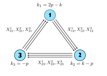
Figure 1: The quiver diagram for Chern-Simons dual of $AdS_{4}\times Y^{p,k}(\mathbb{CP}^{2})$

There are nine chiral multiplets in total which are represented by arrows in the quiver diagram. They interact via a cubic superpotential

$$W=\sum_{i,j,k=1}^{3}\epsilon_{ijk}\text{Tr}(X_{12}^{i}X_{23}^{j}X_{31}^{k}).$$ (21)

Not surprisingly this proposal is very similar to that of $M^{1,1,1}=Y^{2,3}(\mathbb{CP}^{2})$ which is a homogeneous Sasaki-Einstein seven-manifold with $KE_{6}=\mathbb{CP}^{2}\times\mathbb{CP}^{1}$. It is obvious that if $p=2r,k=3r$ the quiver Chern-Simons theory becomes identical to the proposed dual for ${\rm AdS}_{4}\times M^{1,1,1}/\mathbb{Z}_{r}$. This happens when $\kappa=0$, when $H(x)=0$ develops double roots. It is less clear how to see this special arrangement leads to the homogeneous metric, $M^{1,1,1}$, or $Q^{1,1,1}$ when ${\cal M}_{4}=\mathbb{CP}^{1}\times\mathbb{CP}^{1}$. It involves reviving another parameter in the metric which was originally scaled away, and taking a particular scaling limit. For details readers are referred to ref. Gauntlett:2004hh .

The vacuum moduli space $\mathscr{M}_{3}$ of the above ${\cal N}=2$ Chern-Simons theory has been computed in ref. Martelli:2008si . When the toric data is compared to that of $Y^{p,k}(\mathbb{CP}^{2})$, one finds agreement for the range

$$3p/2\leq k\leq 2p.$$ (22)

Outside this region, i.e. if $2p<k<3p$, among the toric data of $\mathscr{M}_{3}$ there is one vertex which lies outside the polytope for $Y^{p,k}(\mathbb{CP}^{2})$ Martelli:2008si . To the best of our knowledge, the dual CFTs for the range of $2p<k<3p$ are not known yet.

Let us consider the lowest-level chiral primary operators which are written purely in terms of the scalar fields of the CFT. They constitute the lowest-lying modes of Kaluza-Klein reduction of 11-dimensional supergravity on $Y^{p,k}$. As usual, the chiral primary operators are gauge singlets and classified up to F-term condition. The simplest ones we can think of are

$$(\mathscr{O}^{3}_{0})^{ijk}=\text{Tr}(X_{12}^{i}X_{23}^{j}X_{31}^{k}).$$ (23)

Due to the F-term conditions the $SU(3)$ indices $i,j,k$ are symmetrized, so these operators are in ${\bf 10}$ of $SU(3)$. Being of the same order as $W$ and BPS, the conformal dimension $\Delta$ and R-charge $R$ are both 2. There is one more global charge we can match against the geometric data, which is the monopole charge number $Q_{m}$. Since we do not have any monopole operator insertion, for $\mathscr{O}^{3}_{0}$ we set $Q_{m}=0$.

In the reconstruction of the geometry of Sasaki-Einstein space, it is crucial to incorporate the monopole operators. The diagonal one $e^{ia}$, which is supersymmetric and does not carry bare conformal dimension or R-charge, has charge vector (for abelian case) exactly the same as the Chern-Simons levels. For the quiver theory of figure 1 it is $(2p-k,k-p,-p)$. It is then easily seen that

$$\mathscr{O}^{k}_{+}=\text{Tr}(e^{ia}X^{k-p}_{12}X^{p}_{31})$$ (24)

is a neutral operator. Note that we are schematic here and the symbol Tr means contracting various indices of $e^{ia},X_{12},$ and $X_{31}$ appropriately so that we have a gauge singlet in the end. We also have suppressed the $SU(3)$ indices but it is understood that they are symmetrized due to F-term condition, like $\mathscr{O}^{3}_{0}$. Being supersymmetric, the conformal dimension and R-charge should be still the same and we set $\Delta=R=r_{+}$. Here $r_{+}$ is not known yet but will be fixed using AdS/CFT correspondence. The monopole number is $Q_{m}=1$.

In the same way we can think of

$$\mathscr{O}_{-}^{3p-k}=\text{Tr}(e^{-ia}X^{2p-k}_{12}X^{p}_{23}),$$ (25)

with $\Delta=R=r_{-}$ and $Q_{m}=-1$. At this stage we only know

$$r_{+}+r_{-}=2p.$$ (26)

One can construct higher-level chiral primary operators by taking symmetric products of the three basic operators (to be precise multiplying the expressions within Tr, and taking the trace after multiplication to have a single-trace operator) given above. And such operators are dual to orbiting particles in the supergravity background of ${\rm AdS}_{4}\times Y^{p,k}$. More concretely, we consider particles moving only along the $U(1)$ fibre in the canonical form. In other words we consider geodesic motions with ansatz $t=\kappa\tau,\,\psi^{\prime}=\omega\tau$ and set all the remaining angles including $x$ to constant. The computation is elementary and we obtain $\kappa=\pm 2\omega$. We restrict to holomorphic expressions of the complex scalar fields and choose $\kappa=2\omega>0$. For our purpose it is important to have the ratios between varioius conserved charges. We define $E$ to be the conjugate momentum for $t$, $J_{\psi^{\prime}}$ as conjugate to $\psi^{\prime}$ etc. For $Y^{p,k}(\mathbb{CP}^{2})$,

$$E:J_{\tilde{\phi}}:J_{\tilde{\psi}}:J_{\phi}:J_{\psi^{\prime}}=1:\frac{3}{4}x\sin^{2}\mu\cos\tilde{\theta}:\frac{3}{4}x\sin^{2}\mu:\frac{1-x}{2}:2.$$ (27)

Note that $x,\mu,\tilde{\theta}$ are constants here. The ratios can take values within a limited range, for instance $0\leq J_{\tilde{\phi}}\leq\tfrac{3}{4}x_{2}E$. On the other hand, for $Y^{p,k}(\mathbb{CP}^{1}\times\mathbb{CP}^{1})$, we obtain

$$E:J_{\phi_{1}}:J_{\phi_{2}}:J_{\phi}:J_{\psi^{\prime}}=1:\frac{x}{2}\cos\theta_{1}:\frac{x}{2}\cos\theta_{2}:\frac{1-x}{2}:2,$$ (28)

where $x,\theta_{1},\theta_{2}$ are constants.

We next consider matching the CFT side data for chiral primaries and the gravity side data from geodesic motion, for $Y^{p,k}(\mathbb{CP}^{2})$. On the CFT side, we have five commuting physical observables which may have non-trivial values for operators such as $\mathscr{O}^{k}_{0},\mathscr{O}_{+}^{k},\mathscr{O}_{-}^{3p-k}$. They are $\Delta,R,Q_{m}$ and also two more charges which determine the $SU(3)$ representation. Let us first identify $\Delta$ with $E$. Then from the fact that $E:J_{\psi^{\prime}}=1:2$ it is obvious we should relate $R=J_{\psi^{\prime}}/2$. Changing $\mu,\tilde{\theta}$ should correspond to assigning different $SU(3)$ indices, since they are among $\mathbb{CP}^{2}$ angles. We will thus identify $J_{\tilde{\phi}},J_{\tilde{\psi}}$ with the Cartan generators of the $SU(3)$ symmetry. It turns out correct to relate $J_{\phi}$ with the monopole number $Q_{m}$. For $x=1$ orbits, we have $Q_{m}=0$ and the duals are without monopole operator insertions. $x=x_{2}$ orbits are in fact dual to operators with maximally possible $e^{ia}$ insertions, like $\mathscr{O}^{k}_{+}$. In the same way we should identify operators like $\mathscr{O}^{3p-k}_{-}$ with $x=x_{1}$ orbits. We provide more concrete $SU(3)$ part identifications and check our mappings with several examples in the following.

Let us first consider $x=1$ cases and try to find out the relation between the highest weights of $SU(3)$ representation and angular momenta of particle solution. For $SU(3)$ we follow the standard convention and use

$$Q_{3}=\frac{1}{2}\begin{pmatrix}1&0&0\\ 0&-1&0\\ 0&0&0\end{pmatrix},\quad Q_{8}=\frac{1}{2\sqrt{3}}\begin{pmatrix}1&0&0\\ 0&1&0\\ 0&0&-2\end{pmatrix},$$ (29)

for fundamental representation. For instance if we consider $\mathscr{O}^{3}_{0}$ with $i=j=k=1$, we obtain $Q_{3}=3/2,Q_{8}=\sqrt{3}/2$. In general for a symmetric product like $\text{Tr}[(X_{12}X_{23}X_{31})^{n}]$ with all $SU(3)$ indices equal to $1$, we would obtain $\Delta=R=2n,Q_{3}=3n/2,Q_{8}=\sqrt{3}n/2$. Now looking at the metric convention for $\mathbb{CP}^{2}$ in eq.(19), we want to identify these operators with orbits at $\mu=\pi/2,\tilde{\theta}=0$. In a similar way, $i=2$ maps to $\mu=\pi/2,\tilde{\theta}=\pi$, and $i=3$ is for $\mu=0$. When we consider the possible values for ratios from the gravity side and the eigenvalues of $Q_{3},Q_{8}$, it is not difficult to conclude that we should identify

$$Q_{3} = J_{\tilde{\phi}},$$ (30)

$$Q_{8} = \sqrt{3}(J_{\tilde{\psi}}+J_{\phi}-\frac{1}{4}J_{\psi^{\prime}}).$$ (31)

This part of the consideration is very similar to the $M^{1,1,1}$ case Kim:2010ck .

Now what about operators with monopoles, like $\mathscr{O}_{+}^{k},\mathscr{O}_{-}^{3p-k}$? As mentioned earlier, we assume $x=x_{2}$ orbits have maximally possible insertions of $e^{ia}$, like $\text{Tr}[(e^{ia}X^{k-p}_{12}X^{p}_{31})^{n}]$. And $x=x_{1}$ orbits are dual to operators like $\text{Tr}[(e^{-ia}X^{2p-k}_{12}X^{p}_{23})^{n}]$. We check this conjecture leads to a nontrivial realization of eq.(26). One can now fix the values $r_{+},r_{-}$ by considering the ratio $J_{\tilde{\phi}}/E$ and $Q_{3}/\Delta$ for $\mathscr{O}_{+}^{k},\mathscr{O}_{-}^{3p-k}$.

$$r_{-}=\frac{2(3p-k)}{3x_{1}},\quad r_{+}=\frac{2k}{3x_{2}}.$$ (32)

One can easily see that this is consistent with eq.(26), with the help of the second identity in eq.(13). We have the same type of consistency when considering $Q_{8}/\Delta$. Finally we need to fix the proportionality coefficient in identifying $J_{\phi}$ with $Q_{m}$. It turns out we should relate

$$Q_{m}=-lJ_{\phi},$$ (33)

which implies $r_{+}=\frac{2}{l(x_{2}-1)},r_{-}=\frac{2}{l(1-x_{1})}$ from the consideration of $\mathscr{O}^{k}_{+},\mathscr{O}^{3p-k}_{-}$. This assignment is easily shown to be identical to eq.(32), using eq.(13).

4 Scalar Laplacian on $Y^{p,k}$

4.1 Scalar Laplacian and Kaluza-Klein reduction

We now turn to the solutions of Laplace equation for $Y^{p,k}$. There are two motivations for doing this. One is as the quantum mechanism on $Y^{p,k}$. In order to explore the AdS/CFT correspondence, in principle we need to quantize the membrane action in the nontrivial background ${\rm AdS}_{4}\times Y^{p,k}$. This is certainly a very nontrivial problem, and one can alternatively tackle quantization of particle motion and try to obtain some (limited) information on M-theory spectrum at quantum level.

Another motivation is as part of the Kaluza-Klein (KK) reduction problem. As an example of ${\rm AdS}_{4}/{\rm CFT}_{3}$ correspondence, one needs to perform the KK computation and obtain the matter fields for four-dimensional supergravity. According to AdS/CFT, these supergravity modes are dual to chiral primary operators in the dual field theory. The entire KK computation is not a trivial task, but we have complete results for $S^{7}$ and other coset manifolds such as $Q^{1,1,1},M^{1,1,1}$ Duff:1986hr ; Pope:1984ig ; Fabbri:1999mk . The space of our interest $Y^{p,k}$ is not a coset nor homogeneous, and the KK spectrum is not dictated by symmetry through group theory computations. Instead of the full analysis, we will consider a simpler subset, i.e. the scalar Laplacian in this paper.

Although the eleven-dimensional supergravity does not have any scalar field, the spectrum of scalar Laplacian makes an appearance in KK computation. On the problem of separating the various Laplace-Beltrami equations for metric tensor and four-form flux, readers are referred to a classic review paper on Kaluza-Klein supergravity by Duff et al. Duff:1986hr . Their computation is summarised in table 5 of Duff:1986hr , and the scalar Laplacian among other things gives rise to the modes called $0^{+(1)}$, with four-dimensional mass

$$m^{2}=\mathscr{E}+44-12\sqrt{\mathscr{E}+9}.$$ (34)

Our convention is $\Box Y=-\mathscr{E}Y$ with harmonic functions $Y$. We need to recall that in the convention of ref. Duff:1986hr the conformal coupling term of scalar fields with Ricci scalar is written separately. Then the above relation implies the existence of CFT operators with conformal dimension

$$4\Delta(\Delta-3)=\mathscr{E}+36-12\sqrt{\mathscr{E}+9},$$ (35)

according to the standard AdS/CFT prescription.

As a warm-up, let us first consider the homogeneous Sasaki-Einstein manifolds and check eq.(35) leads to consistent predictions on dual CFT.

1. $S^{7}$

   For round $S^{7}$ with unit radius, the eigenvalues are $\mathscr{E}=j(j+6),\,\,j=0,1,2,\ldots$, for rank-$j$ totally symmetric representation of $SO(8)$. For dual operators we have $\Delta=j/2$. This is consistent with the fact that there are (allowing insertions of monopole operators) effectivly eight scalar fields $X^{I}\,(I=1,2,\ldots,8)$ with $\Delta=1/2$ in ABJM model with Chern-Simons level $k=1$. For instance, a chiral primary operator is written as

   $$S_{I_{1}I_{2}\cdots I_{j}}\text{Tr}(X^{I_{1}}X^{I_{2}}\cdots X^{I_{j}}),\quad\quad\Delta=j/2,$$ (36)

   where $S_{I_{1}I_{2}\cdots}$ is symmetric and traceless.

2. $Q^{1,1,1}$

   The eigenvalues are computed for instance in Pope:1984ig ,

   $$\mathscr{E}=8(j_{1}(j_{1}+1)+j_{2}(j_{2}+1)+j_{3}(j_{3}+1)-s^{2}),$$ (37)

   where $s=0,\pm 1/2,\pm 1,\ldots$ and $j_{1},j_{2},j_{3}=|s|,|s|+1,|s|+2,\ldots$. The lowest-lying nontrivial mode is given as $j_{1}=j_{2}=j_{3}=s=1/2$, or $(2,2,2)$ representation of the global symmetry $SU(2)\times SU(2)\times SU(2)$, with $\Delta=1$. There exist at least two proposals for CFT dual of (orbifolded) ${\rm AdS}_{4}\times Q^{1,1,1}$, see for instance Franco:2009sp ; Aganagic:2009zk . And both of them exhibit chiral primary operators in $(2j+1,2j+1,2j+1)$ with $\Delta=2j$. The corresponding bulk scalar modes are identified as eigenfunction of Laplace operator with $j_{1}=j_{2}=j_{3}=s=j$.

3. $M^{1,1,1}$

   The eigenvalues are given as Pope:1984ig

   $$\mathscr{E}=\frac{16}{3}(k^{2}+2(1+3|s|)k+6|s|))+8(j(j+1)-4s^{2})+64s^{2},$$ (38)

   where $s=0,\pm\tfrac{1}{2},\pm 1,\cdots$, $j=2|s|,2|s|+1,\cdots$, and $k=0,1,2,\cdots$. $M^{1,1,1}$ has $SU(3)\times SU(2)\times U(1)$ symmetry, and $j$ determines the $SU(2)$ representation, $s$ is for the $U(1)$ charge, and $k,s$ together determine $SU(3)$ representaion. In particular, for $s>0$ the eigenmodes are in $(k,k+6s)$ of $SU(3)$ and if $s<0$ the $SU(3)$ representation is in $(k+6|s|,k)$ Pope:1984ig . The basic chiral primary operator for dual CFT is in ${\bf 10}$, or rank-3 symmetric tensor which can be also written as $(0,3)$-representation. At the same time they are a triplet of $SU(2)$ and have $\Delta=2$. This particular set of operators can be mapped to eigenmodes with $k=0,j=1,$ and $s=1/2$. Then we have $\mathscr{E}=40$ and can match with $\Delta=2$. More generally, if we consider symmetric products they are dual to the modes in $(0,6s)$-rep of $SU(3)$ and spin-$2s$ representation of $SU(2)$, for $s=\tfrac{1}{2},1,\tfrac{3}{2},\ldots$.

4.2 Separation of variables and ODE with five singularities

4.2.1 $\mathbb{CP}^{1}\times\mathbb{CP}^{1}$ Base

One can begin with the computation of scalar Laplace operator for the seven-manifold.

$$\square= \frac{4}{x^{2}}\partial_{x}\biggl{(}x^{2}U(x)\partial_{x}\biggr{)}+\frac{8}{x}\sum_{i=1}^{2}\biggl{[}\frac{1}{\sin\theta_{i}}\partial_{\theta_{i}}(\sin\theta_{i}\partial_{\theta_{i}})+\biggl{(}\frac{1}{\sin\theta_{i}}\partial_{\phi_{i}}+\cot\theta_{i}\partial_{\psi}\biggr{)}^{2}\biggr{]}$$

$$+\frac{16}{U(x)}\biggl{(}\partial_{\alpha}+(1-x)(\partial_{\psi}-\partial_{\alpha})\biggr{)}^{2}+16(\partial_{\psi}-\partial_{\alpha})^{2}.$$ (39)

As usual we separate the variables by writing putative eigenmodes as

$$\Phi(x,\theta_{1},\theta_{2},\phi_{1},\phi_{2},\psi,\alpha)=X(x)\Theta_{1}(\theta_{1})\Theta_{2}(\theta_{2})\text{exp}\biggl{[}i\biggl{(}N_{\phi_{1}}\phi_{1}+N_{\phi_{2}}\phi_{2}+N_{\psi}\psi+\displaystyle\frac{N_{\alpha}}{l}\alpha\biggr{)}\biggr{]},$$ (40)

One first solves the $\mathbb{CP}^{1}$ parts one by one, using

$$\biggl{[}\displaystyle\frac{1}{\sin\theta_{1}}\partial_{\theta_{1}}(\sin\theta_{1}\partial_{\theta_{1}}) +\biggl{(}\displaystyle\frac{N_{\phi_{1}}}{\sin\theta_{1}}+N_{\psi}\cot\theta_{1}\biggr{)}^{2}\biggr{]}\Theta_{1}=-\biggl{(}j_{1}(j_{1}+1)-N_{\psi}^{2}\biggr{)}\Theta_{1}$$ (41)

and also in a similar way for $\Theta_{2}$. The $SU(2)$ quantum numbers $j_{1},j_{2}$ can take values $|N_{\psi}|,|N_{\psi}|+1,\cdots$. Now the Laplace equation $\Box\Phi=-\mathscr{E}\Phi$ is reduced to a second order ordinary differential equation (ODE) for $X(x)$,

$$\frac{4}{x^{2}}\displaystyle\frac{\text{d}}{\text{d}x}\biggl{(}x^{2}U(x)\displaystyle\frac{\text{d}}{\text{d}x}X(x)\biggr{)}-\biggl{\{}\frac{8}{x}\biggl{(}j_{1}(j_{1}+1)+j_{2}(j_{2}+1)-2N_{\psi}^{2}\biggr{)}$$

$$+\frac{16}{U(x)}\biggl{(}\frac{N_{\alpha}}{l}+(1-x)\biggl{(}N_{\psi}-\frac{N_{\alpha}}{l}\biggr{)}\biggr{)}^{2}+16\biggl{(}N_{\psi}-\frac{N_{\alpha}}{l}\biggr{)}^{2}-\mathscr{E}\biggr{\}}X(x)=0.$$ (42)

4.2.2 $\mathbb{CP}^{2}$ Base

It is straightforward to compute the Laplace operator.

$$\square= \frac{4}{x^{2}}\partial_{x}\biggl{(}x^{2}U(x)\partial_{x}\biggr{)}+\frac{4}{x}\biggl{\{}\frac{1}{3\sin^{3}\mu\cos\mu}\partial_{\mu}(\sin^{3}\mu\cos\mu\partial_{\mu})+\frac{4}{3\sin^{2}\mu}\biggl{[}\frac{1}{\sin\tilde{\theta}}\partial_{\tilde{\theta}}(\sin\tilde{\theta}\partial_{\tilde{\theta}})$$

$$\quad+\biggl{(}\frac{1}{\sin\tilde{\theta}}\partial_{\tilde{\phi}}-\cot\tilde{\theta}\partial_{\tilde{\psi}}\biggr{)}^{2}\biggr{]}+\frac{4}{3\sin^{2}\mu\cos^{2}\mu}\biggl{(}\partial_{\tilde{\psi}}-\frac{3}{2}\sin^{2}\mu\partial_{\psi}\biggr{)}^{2}\biggr{\}}$$

$$\quad+\frac{16}{U(x)}\biggl{(}\partial_{\alpha}+(1-x)(\partial_{\psi}-\partial_{\alpha})\biggr{)}^{2}+16(\partial_{\psi}-\partial_{\alpha})^{2}.$$ (43)

And we again employ the technique of separating the variables by assuming an eigenfunction of the following form.

$$\Phi(x,\mu,\tilde{\theta},\tilde{\phi},\tilde{\psi},\psi,\alpha)={{X}(x){M}(\mu)\Theta(\tilde{\theta})}\text{exp}\biggl{[}i\biggl{(}N_{\tilde{\phi}}\tilde{\phi}+\displaystyle\frac{N_{\tilde{\psi}}}{2}\tilde{\psi}+N_{\psi}\psi+\displaystyle\frac{N_{\alpha}}{l}\alpha\biggr{)}\biggr{]}.$$ (44)

Now some of the partial derivatives turn into integration constants, and then we solve the $\mathbb{CP}^{2}$ part. The $\mathbb{CP}^{1}\subset\mathbb{CP}^{2}$ should be tackled first, and we can effectively substitute

$$\frac{1}{\sin\tilde{\theta}}\partial_{\tilde{\theta}}(\sin\tilde{\theta}\partial_{\tilde{\theta}})+\biggl{(}\frac{1}{\sin\tilde{\theta}}\partial_{\tilde{\phi}}-\cot\tilde{\theta}\partial_{\tilde{\psi}}\biggr{)}^{2}\longrightarrow-j(j+1)+\frac{N^{2}_{\tilde{\psi}}}{4},$$ (45)

where $N_{\tilde{\psi}}$ is integer, and $j=|N_{\tilde{\psi}}|/2,|N_{\tilde{\psi}}|/2+1,\cdots.$ The equation for $M(\mu)$ should complete the solution for $\mathbb{CP}^{2}$ part. The result is determined by the group theory for $SU(3)$, simply an eigenvalue of quadratic Casimir operator. We obtain

$$\displaystyle\frac{1}{3\sin^{3}\mu\cos\mu}\partial_{\mu}(\sin^{3}\mu\cos\mu\partial_{\mu}) -\displaystyle\frac{4j(j+1)-N_{\tilde{\psi}}^{2}}{3\sin^{2}\mu}-\frac{(N_{\tilde{\psi}}-3N_{\psi}\sin^{2}\mu)^{2}}{3\sin^{2}\mu\cos^{2}\mu}$$

$$\longrightarrow-\displaystyle\frac{4}{3}(M_{1}+M_{2}+M_{1}M_{2}),$$ (46)

$M_{1},M_{2}$ determine the relevant $SU(3)$ representation. They range as $M_{1}=s$, $M_{2}=s+3N_{\psi}$ and $s=0,1,\cdots.$ Now we have an ordinary differential equation for $X(x)$,

$$\frac{4}{x^{2}}\displaystyle\frac{\text{d}}{\text{d}x}\biggl{(}x^{2}U(x)\displaystyle\frac{\text{d}}{\text{d}x}X(x)\biggr{)}-\biggl{\{}\frac{4}{x}\displaystyle\frac{4}{3}\Big{(}s+(s+3N_{\psi})+s(s+3N_{\psi})\Big{)}$$

$$+\frac{16}{U(x)}\biggl{(}\frac{N_{\alpha}}{l}+(1-x)\biggl{(}N_{\psi}-\frac{N_{\alpha}}{l}\biggr{)}\biggr{)}^{2}+16\biggl{(}N_{\psi}-\frac{N_{\alpha}}{l}\biggr{)}^{2}-\mathscr{E}\biggr{\}}X(x)=0.$$ (47)

One can easily see that, not surprisingly, the ODEs eq.(42) and eq.(47) are of the same form apart from the integration constants from ${\cal M}_{4}$. Let us introduce a new constant

$$Q_{R} = 2(N_{\psi}-\frac{N_{\alpha}}{l}),$$ (48)

which is the eigenvalue for $i\partial_{\psi^{\prime}}/2$, so gives us the R-charge of the solution. On the other hand $N_{\alpha}$ is integral and since $il\partial_{\alpha}$ is related to monopole charge, we can interpret it as $Q_{m}=N_{\alpha}$. To simplify the ODE, we introduce a shorthand notation for the eigenvalues of four-dimensional Laplacian as follows

$$C=\left\{\begin{array}[]{ll}\displaystyle\frac{4}{3}\Big{(}s+(s+3N_{\psi})+s(s+3N_{\psi})\Big{)},&\text{for $\mathcal{M}_{4}=\mathbb{CP}^{2}$}.\cr 2\Big{(}j_{1}(j_{1}+1)+j_{2}(j_{2}+1)-2N_{\psi}^{2}\Big{)},&\text{for $\mathcal{M}_{4}=\mathbb{CP}^{1}\times\mathbb{CP}^{1}$}.\end{array}\right.$$ (49)

Obvious $C$ is determined by the representation of the solution for non-R global symmetry.

Then the ODE can be written as follows,

$$\displaystyle\frac{\text{d}^{2}}{\text{d}x^{2}}X(x)+\sum^{4}_{i=1}\frac{1}{x-x_{i}}\displaystyle\frac{\text{d}}{\text{d}x}X(x)+\frac{1}{H(x)}\biggl{\{}-\frac{1}{9}\biggl{(}6\frac{N_{\alpha}}{l}-Q_{R}\biggr{)}^{2}$$

$$\quad\quad+x\biggl{(}C+\frac{2Q_{R}}{3}\biggl{(}6\frac{N_{\alpha}}{l}+Q_{R}\biggr{)}\biggr{)}-\frac{\mathscr{E}}{4}x^{2}-\sum^{4}_{i=1}\frac{\alpha_{i}^{2}H^{\prime}(x_{i})}{x-x_{i}}\biggr{\}}X(x)=0.$$ (50)

As defined earlier $H(x)=x^{4}-\frac{4}{3}x^{3}-\frac{\kappa}{3}=\prod_{i=1}^{4}(x-x_{i})$. Among the roots $x_{1},x_{2}$ are real but $x_{3},x_{4}$ are complex-valued. This ODE has five regular singular points on complex plane, at $x=x_{1},x_{2},x_{3},x_{4},$ and $\infty$. The parameters $\alpha_{i}$ are given as for instance

$$\alpha_{1}=-\frac{\Big{(}4\displaystyle\frac{N_{\alpha}}{l}+2(1-x_{1})Q_{R}\Big{)}x_{1}^{2}}{2(x_{1}-x_{2})(x_{1}-x_{3})(x_{1}-x_{4})}=\frac{Q_{R}}{4}-\frac{N_{\alpha}}{2l}\frac{1}{x_{1}-1},$$ (51)

and similarly for others. Note that $\alpha_{3},\alpha_{4}$ are complex-valued but they are complex conjugate to each other. One can easily show

$$\sum\alpha_{i}=Q_{R}.$$ (52)

The asymptotic behavior of $X(x)$ near $x=x_{i}$ is given as $X(x)\sim(x-x_{i})^{\alpha_{i}}$. If we extract the asymptotic behavior by setting

$$X(x)=\prod^{4}_{i=1}(x-x_{i})^{\alpha_{i}}f(x),$$ (53)

we have the following ODE in standard form

$$\frac{\text{d}^{2}}{\text{d}x^{2}}f(x)+\sum^{4}_{i=1}\frac{1+2\alpha_{i}}{x-x_{i}}\frac{\text{d}}{\text{d}x}f(x)+\frac{\alpha x^{2}+\beta x}{\prod_{i=1}^{4}(x-x_{i})}f(x)=0.$$ (54)

The parameters $\alpha,\beta$ are given as

$$\alpha =Q_{R}(Q_{R}+3)-\frac{\mathscr{E}}{4},$$ (55)

$$\beta =C-4\frac{N_{\alpha}}{l}-2Q_{R}.$$ (56)

4.3 Explicit solutions and BPS conditions

In this section we will present simple solutions for $f(x)$ which are either constant or linear in $x$. We also try to give their interpretation as operators in quiver gauge theory figure 1, for ${\cal M}_{4}=\mathbb{CP}^{2}$.

4.3.1 Constant solutions and Chiral Primaries

Obviously $f(x)=const.$ becomes a solution if $\alpha=\beta=0$. $\alpha=0$ implies $\Delta=Q_{R}$, which is the familiar supersymmetry condition for chiral primaries that conformal dimension should be equal to R-charge. Then $\beta=0$ leads to $C=4N_{\psi}$. Since $N_{\psi}=Q_{R}/2+N_{\alpha}/l$, this condition relates the representation of non-R flavor symmetry with monopole number and R-charge.

We can easily check that these conditions indeed account for the chiral primary operators of $Y^{p,k}(\mathbb{CP}^{2})$, as follows. Let us start with the case $N_{\psi}=1$. Then $\beta=0$, or equivalently $C=4$ implies we should set $s=0$, i.e. the $SU(3)$ representation is in $(0,3)$, i.e. ${\bf 10}$. If we further set $N_{\alpha}=0$ then $Q_{R}=2$. Now we look at $\alpha=0$ and see $\Delta=2$. This particular state obviously corresponds to $\mathscr{O}^{3}_{0}=\text{Tr}(X_{12}X_{23}X_{31})$. We can also find duals for other operators. For $\mathscr{O}_{+}^{k}$, we need to choose $N_{\psi}=k/3,N_{\alpha}=1$ and $Q_{R}=r_{+}$. Or for $\mathscr{O}_{-}^{3p-k}$, one finds $N_{\psi}=(3p-k)/3,N_{\alpha}=-1,Q_{R}=r_{-}$ do the job. For doing this, we can make use of the following identities which can be derived from eq.(13).

$$l=\frac{hx_{2}}{k(x_{2}-1)}=\frac{hx_{1}}{(k-hp)(x_{1}-1)}.$$ (57)

Similarly we can describe all higher composite operators, which are purely made of scalar operators with numerous insertions of monopole operators $e^{\pm ia}$.

Now it should be clear that we can find states dual to the chiral primary operators such as listed in Sec.3, but how do we know that other assignments of quantum numbers are prohibited? For instance, what would happen if we considered $N_{\psi}=1,N_{\alpha}=1$ instead of $N_{\psi}=1,N_{\alpha}=0$ which gives us $\mathscr{O}^{3}_{0}$? The correct quantization is given by regularity of wavefunction, of course. And for that matter, in practice we need to consider two things here. One is the correct periodicity for various angles in the metric, especially $\alpha,\psi$. The other is the convergence of the eigenmode at north and south pole of squashed $S^{2}$, i.e. $x=x_{1},x_{2}$.

A systematic way of determining the correct periodicity condition, or single-valuedness of the wavefunction, is to use toric geometry. $Y^{p,k}$ spaces are toric when we choose the four-dimensional Kähler-Einstein base ${\cal M}_{4}$ as toric. It is certainly the case for ${\cal M}_{4}=\mathbb{CP}^{2}$ or $\mathbb{CP}^{1}\times\mathbb{CP}^{1}$. More precisely, the metric cone of $Y^{p,k}$ is toric, in other words it is a complex four-dimensional space and can be expressed as $U(1)^{4}$ fibration over a convex rational polyhedral cone. In order to compute the toric data it is crucial to establish a basis for an effectively acting torus action $\mathbb{T}^{4}$. The result is reported in ref. Martelli:2008rt , and for our purpose readers are asked to bring their attention to the Killing vectors $e_{3},e_{4}$ in eq.(3.7) of Martelli:2008rt . In our notation they are

$$e_{3}=\frac{\partial}{\partial\psi}-\frac{kl}{3}\frac{\partial}{\partial\alpha},\quad e_{4}=l\frac{\partial}{\partial\alpha}.$$ (58)

The fact that they are effectively acting means that their eigenvalues should be $i$ times an integer. In particular, it implies $N_{\alpha}=Q_{m}$ should be an integer, and so should $N_{\psi}-kN_{\alpha}/3$. We should also check if $X(x)=f(x)\prod(x-x_{i})^{\alpha}$ stays finite at $x=x_{1},x_{2}$. For constant $f(x)$, we should simply avoid the cases with negative $\alpha_{1},\alpha_{2}$.

Let us use a specific example of $(p,k)=(4,7)$ here, in order to illustrate that the above conditions really pin down the spectrum BPS operators. One can easily compute $\alpha_{1}=\tfrac{1}{2}(N_{\psi}+\frac{5}{3}N_{\alpha})$ and $\alpha_{2}=\frac{1}{2}(N_{\psi}-\tfrac{7}{3}N_{\alpha})$ . Since $N_{\alpha}$ is integral, we start with $N_{\alpha}=0$. Then $N_{\psi}$ should be non-negative to guarantee $\alpha_{1},\alpha_{2}\geq 0$. These states are dual to $\text{Tr}[(X_{12}X_{23}X_{31})^{N_{\psi}}]$. Let us now consider $N_{\alpha}=1$. Then from the consideration of $e_{3}$ we see $N_{\psi}\in\mathbb{Z}+\tfrac{7}{3}$. And since we want $\alpha_{2}\geq 0$, we can only have $N_{\psi}=\tfrac{7}{3},\tfrac{10}{3},\tfrac{13}{3},\cdots$. One can easily compute $C,Q_{R}$ for these solutions, and convince oneself that they are dual to $\text{Tr}[(e^{ia}X_{12}^{2p-k}X_{23}^{p})(X_{12}X_{23}X_{31})^{N_{\psi}-7/3}]$. A similar argument holds for $N_{\alpha}=-1$ etc.

We can do something similar with ${\cal M}_{4}=\mathbb{CP}^{1}\times\mathbb{CP}^{1}$, although we do not know the dual Chern-Simons theory yet. From toric data we need integrality of eigenvalues for the following Killing vectors (see eq.(3.25) of ref. Martelli:2008rt ),

$$e_{3}=\frac{\partial}{\partial\psi}-\frac{kl}{2}\frac{\partial}{\partial\alpha},\quad e_{4}=l\frac{\partial}{\partial\alpha}.$$ (59)

And we also require $\alpha_{1}=\tfrac{1}{2}(N_{\psi}+\tfrac{2p-k}{2}N_{\alpha}),\,\alpha_{2}=\tfrac{1}{2}(N_{\psi}-\tfrac{k}{2}N_{\alpha})$ be non-negative. Now let us consider the condition $\beta=0$. We immediately see that the simplest way of satisfying $C=4N_{\psi}$ is $j_{1}=j_{2}=N_{\psi}$. If we again start with $N_{\alpha}=0$, $N_{\psi}$ should be an integer and we may conjecture there should be BPS operators $\mathscr{O}^{n}_{0}$ with $j_{1}=j_{2}=N_{\psi}=n$ and $Q_{R}=2n$. Next we consider $N_{\alpha}=1$, and from $\alpha_{2}\geq 0$ we conjecture there are operators $\mathscr{O}_{+}^{k/2+n}\,(n=0,1,2,\cdots)$ with $j_{1}=j_{2}=N_{\psi}=\tfrac{k}{2}+n$ and $Q_{R}=k-2/l+2n$. And for $N_{\alpha}=-1$, in a similar way we obtain $j_{1}=j_{2}=N_{\psi}=p-k/2+n$ with $n=0,1,2,\cdots$ from $\alpha_{1}\geq 0$. R-charge is given as $Q_{R}=2p-k+2n+2/l$, and we can call these states $\mathscr{O}^{p-k/2+n}_{-}$. One can certainly continue with other values of $N_{\alpha}$.

4.3.2 First excited states: linear $f(x)$

Although it seems too difficult to find a complete set of solutions to eq. (54), it turns out we can find some excited states where $f(x)$ is a linear function. Let us try $f(x)=x+a$, upon which the ODE becomes

$$\sum\frac{1+2\alpha_{i}}{x-x_{i}}+\frac{\alpha x^{2}+\beta x}{H(x)}(x+a)=0.$$ (60)

One may make use of the following identities,

$$H(x)\sum\frac{1}{x-x_{i}} = H^{\prime}(x)=4x^{2}(x-1),$$ (61)

$$H(x)\sum\frac{\alpha_{i}}{x-x_{i}} = x^{2}\left(Q_{R}x-Q_{R}-\frac{2N_{\alpha}}{l}\right).$$ (62)

Then it is a simple matter to solve eq. (60). One first needs to set $\alpha=-2Q_{R}-4$, which implies $\Delta=Q_{R}+1$. For $\beta$, there are two possibilities. $\beta=0$ which gives $C=2Q_{R}+4N_{\alpha}/l$, or $\beta=2(Q_{R}+2N_{\alpha}/l)+4$ which means $C=4Q_{R}+8N_{\alpha}/l+4$.

Having a simple definite relation between $\Delta$ and $Q_{R}$, we expect the duals are also BPS, and even in the same supermultiplet as constant solutions. Candidate operators can be made with insertions of fermion bilinears, which have a different ratio of conformal dimension and R-charge than scalar fields. We can again consider different values of monopole number $N_{\alpha}$ and check if the wavefunction is single-valued and finite-valued for different representations of $SU(3)$ or $SU(2)\times SU(2)$, but we do not go into further details here.

5 Discussions

In this paper we have studied the AdS/CFT duality relation for M-theory background AdS${}_{4}\times{\cal M}_{7}$, where ${\cal M}_{7}$ is an inhomogeneous Sasaki-Einstein manifold. For concreteness we have chosen cohomogeneity-1 examples, $Y^{p,k}(\mathbb{CP}^{2})$ and $Y^{p,k}(\mathbb{CP}^{1}\times\mathbb{CP}^{1})$. Using simple geodesic motions we have established a precise mapping between supergravity and field theory, and through scalar Laplace equation we have seen how chiral primary operators are realized as wavefunctions of quantum mechanics.

The issues covered in this paper are admittedly rather limited. First of all, we have not tried a full treatise of Kaluza-Klein reduction involving the metric, four-form and gravitino fields. We have only studied scalar Laplacian and certainly it is very desirable to extend to the entire action. Even for scalar Laplacian, we managed to obtain only some of the lowest-lying modes. In fact one can check if there are higher-order polynomial solutions for $f(x)$ to eq.(54), but when one tries a quadratic polynomial for $f(x)$ it is easy to see that it leads to inconsistency and there is no such solution. Due to supersymmetry, we expect there should exist higher modes with $\Delta=Q_{R}+2,Q_{R}+3,\cdots$, and it will be very interesting to construct such solutions explicitly.

$Y^{p,k}$ manifolds including homogeneous ones as special cases certainly do not exhaust all explicit Sasaki-Einstein 7-manifolds known to us. There exist higher-cohomogeneity examples such as $L^{p,q,r_{1},r_{2}}$ in seven dimensions, constructed in Cvetic:2005ft ; Cvetic:2005vk . Back to five-dimensions, the gauge duals for ${\rm AdS}_{5}\times L^{p,q,r}$ were identified in refs. Franco:2005sm ; Butti:2005sw , the geodesic motions were studied in Benvenuti:2005ja , while the scalar Laplace equation was studied in Oota:2005mr . We hope to be able to analyze the toric geometry, and the Chern-Simons duals of $L^{p,q,r_{1},r_{2}}$ manifolds and compare the membrane dynamics against the CFT spectra.

- (1) J. Bagger and N. Lambert, Gauge Symmetry and Supersymmetry of Multiple M2-Branes, Phys. Rev. D77 (2008) 065008, [arXiv:0711.0955].
- (2) O. Aharony, O. Bergman, D. L. Jafferis, and J. Maldacena, superconformal Chern-Simons-matter theories, M2-branes and their gravity duals, JHEP 10 (2008) 091, [arXiv:0806.1218].
- (3) Y. Imamura and K. Kimura, On the moduli space of elliptic Maxwell-Chern-Simons theories, Prog. Theor. Phys. 120 (2008) 509–523, [arXiv:0806.3727].
- (4) D. Martelli and J. Sparks, Moduli spaces of Chern-Simons quiver gauge theories and , Phys. Rev. D78 (2008) 126005, [arXiv:0808.0912].
- (5) A. Hanany and A. Zaffaroni, Tilings, Chern-Simons Theories and M2 Branes, JHEP 10 (2008) 111, [arXiv:0808.1244].
- (6) K. Ueda and M. Yamazaki, Toric Calabi-Yau four-folds dual to Chern-Simons-matter theories, JHEP 12 (2008) 045, [arXiv:0808.3768].
- (7) S. Franco, I. R. Klebanov, and D. Rodriguez-Gomez, M2-branes on Orbifolds of the Cone over , JHEP 08 (2009) 033, [arXiv:0903.3231].
- (8) D. Martelli and J. Sparks, duals from M2-branes at hypersurface singularities and their deformations, JHEP 12 (2009) 017, [arXiv:0909.2036].
- (9) F. Benini, C. Closset, and S. Cremonesi, Chiral flavors and M2-branes at toric CY4 singularities, JHEP 02 (2010) 036, [arXiv:0911.4127].
- (10) S. S. Gubser, I. R. Klebanov, and A. M. Polyakov, A semi-classical limit of the gauge/string correspondence, Nucl. Phys. B636 (2002) 99–114, [hep-th/0204051].
- (11) A. A. Tseytlin, Semiclassical strings and AdS/CFT, hep-th/0409296.
- (12) P. Bozhilov, Integrable systems from membranes on , Fortsch. Phys. 56 (2008) 373–379, [arXiv:0711.1524].
- (13) C. Ahn and P. Bozhilov, Finite-size effects of Membranes on , JHEP 08 (2008) 054, [arXiv:0807.0566].
- (14) P. Bozhilov and R. C. Rashkov, On the multi-spin magnon and spike solutions from membranes, Nucl. Phys. B794 (2008) 429–441, [arXiv:0708.0325].
- (15) C. N. Pope, Harmonic Expansions on Solutions of Supergravity with or Symmetry, Class. Quant. Grav. 1 (1984) L91.
- (16) M. J. Duff, B. E. W. Nilsson, and C. N. Pope, Kaluza-Klein Supergravity, Phys. Rept. 130 (1986) 1–142.
- (17) J. Kim, N. Kim, and J. H. Lee, Rotating Membranes in , JHEP 03 (2010) 122, [arXiv:1001.2902].
- (18) J. H. Lee, S. Kim, J. Kim, and N. Kim, Probing Non-Toric Geometry with Rotating Membranes, Nucl. Phys. B838 (2010) 238–252, [arXiv:1003.6111].
- (19) N. Kim and J. H. Lee, Multi-Spin Membrane Solutions in , Talk given at Korean Physical Society meeting, CECO, Changwon, 21-23 Oct 2009.
- (20) J. P. Gauntlett, D. Martelli, J. Sparks, and D. Waldram, Sasaki-Einstein metrics on , Adv. Theor. Math. Phys. 8 (2004) 711–734, [hep-th/0403002].
- (21) D. Martelli and J. Sparks, Toric geometry, Sasaki-Einstein manifolds and a new infinite class of AdS/CFT duals, Commun. Math. Phys. 262 (2006) 51–89, [hep-th/0411238].
- (22) K. A. Intriligator and B. Wecht, The exact superconformal R-symmetry maximizes a, Nucl. Phys. B667 (2003) 183–200, [hep-th/0304128].
- (23) D. Martelli, J. Sparks, and S.-T. Yau, The geometric dual of a-maximisation for toric Sasaki- Einstein manifolds, Commun. Math. Phys. 268 (2006) 39–65, [hep-th/0503183].
- (24) M. Bertolini, F. Bigazzi, and A. L. Cotrone, New checks and subtleties for AdS/CFT and a- maximization, JHEP 12 (2004) 024, [hep-th/0411249].
- (25) S. Benvenuti, S. Franco, A. Hanany, D. Martelli, and J. Sparks, An infinite family of superconformal quiver gauge theories with Sasaki-Einstein duals, JHEP 06 (2005) 064, [hep-th/0411264].
- (26) D. Berenstein, C. P. Herzog, P. Ouyang, and S. Pinansky, Supersymmetry Breaking from a Calabi-Yau Singularity, JHEP 09 (2005) 084, [hep-th/0505029].
- (27) S. Franco, A. Hanany, F. Saad, and A. M. Uranga, Fractional Branes and Dynamical Supersymmetry Breaking, JHEP 01 (2006) 011, [hep-th/0505040].
- (28) M. Bertolini, F. Bigazzi, and A. L. Cotrone, Supersymmetry breaking at the end of a cascade of Seiberg dualities, Phys. Rev. D72 (2005) 061902, [hep-th/0505055].
- (29) E. Caceres, M. N. Mahato, L. A. Pando Zayas, and V. J. G. Rodgers, Toward NS5 Branes on the Resolved Cone over , arXiv:1007.3719.
- (30) J. P. Gauntlett, D. Martelli, J. F. Sparks, and D. Waldram, A new infinite class of Sasaki-Einstein manifolds, Adv. Theor. Math. Phys. 8 (2006) 987–1000, [hep-th/0403038].
- (31) D. Martelli and J. Sparks, Notes on toric Sasaki-Einstein seven-manifolds and , JHEP 11 (2008) 016, [arXiv:0808.0904].
- (32) S. Benvenuti and M. Kruczenski, Semiclassical strings in Sasaki-Einstein manifolds and long operators in gauge theories, JHEP 10 (2006) 051, [hep-th/0505046].
- (33) H. Kihara, M. Sakaguchi, and Y. Yasui, Scalar Laplacian on Sasaki-Einstein manifolds , Phys. Lett. B621 (2005) 288–294, [hep-th/0505259].
- (34) D. Fabbri, P. Fre, L. Gualtieri, and P. Termonia, M-theory on : The complete spectrum from harmonic analysis, Nucl. Phys. B560 (1999) 617–682, [hep-th/9903036].
- (35) M. Aganagic, A Stringy Origin of M2 Brane Chern-Simons Theories, Nucl. Phys. B835 (2010) 1–28, [arXiv:0905.3415].
- (36) M. Cvetic, H. Lu, D. N. Page, and C. N. Pope, New Einstein-Sasaki spaces in five and higher dimensions, Phys. Rev. Lett. 95 (2005) 071101, [hep-th/0504225].
- (37) M. Cvetic, H. Lu, D. N. Page, and C. N. Pope, New Einstein-Sasaki and Einstein spaces from Kerr-de Sitter, JHEP 07 (2009) 082, [hep-th/0505223].
- (38) S. Franco et. al., Gauge theories from toric geometry and brane tilings, JHEP 01 (2006) 128, [hep-th/0505211].
- (39) A. Butti, D. Forcella, and A. Zaffaroni, The dual superconformal theory for L(p,q,r) manifolds, JHEP 09 (2005) 018, [hep-th/0505220].
- (40) S. Benvenuti and M. Kruczenski, From Sasaki-Einstein spaces to quivers via BPS geodesics: , JHEP 04 (2006) 033, [hep-th/0505206].
- (41) T. Oota and Y. Yasui, Toric Sasaki-Einstein manifolds and Heun equations, Nucl. Phys. B742 (2006) 275–294, [hep-th/0512124].