Numerical Resolution near $t=0$ of Nonlinear Evolution Equations in the Presence of Corner Singularities in Space Dimension 1

Abstract

The incompatibilities between the initial and boundary data will cause singularities at the time–space corners, which in turn adversely affect the accuracy of the numerical schemes used to compute the solutions. We study the corner singularity issue for nonlinear evolution equations in 1D, and propose two remedy procedures that effectively recover much of the accuracy of the numerical scheme in use. Applications of the remedy procedures to the 1D viscous Burgers equation, and to the 1D nonlinear reaction–diffusion equation are presented. The remedy procedures are applicable to other nonlinear diffusion equations as well.

Dedicated to the memory of David Gottlieb

1 Introduction

It is well known in the mathematics community that smooth boundary and initial data do not guarantee smooth solutions to the initial-boundary value problems of time-dependent PDEs. Even if the existence and uniqueness of the solution are proved and all the given data are as smooth as desired, then, in order for the solution to be smooth near $t=0$, it is necessary and sufficient that the boundary data and the initial data satisfy an infinite set of so-called compatibility conditions. See [9, 10, 11, 12, 13, 14, 15, 17], and below.

When the boundary and initial data fail to satisfy some of the compatibility conditions, singularities may occur at the corner of the time and spatial axes. In some cases, for simple problems, this is not a critical issue, because the singularity is short-lived.

However in recent years the issue of the compatibility conditions for the initial boundary value problems of time-dependent PDEs started to receive attention in the numerical simulation community, because larger and more complex problems are handled thanks to the ever–growing computing power that is available. This produces a need to better understand what happens during the short initial period for certain physical processes. Boyd and Flyer [3] analyzed the connection between incompatibility and the rate of convergence of Chebyshev spectral series, and discussed the remedy procedure of smoothing the initial conditions. Flyer and Swarztrauber [8] studied the effect of the incompatibilities on the convergence rate of spectral and finite difference methods. Flyer and Fornberg [6] proposed a remedy procedure, based on the idea of singular corner functions, for the heat equation, and for variable coefficient convection–diffusion equations as well. Flyer and Fornberg [7] studied the corner basis functions for some dispersive equations. Bieniasz [2] modified the remedy procedure proposed by Flyer and Fornberg [6], and applied it to a diffusion-reaction system arising from electrochemistry.

In this article we study, from a numerical point of view, the compatibility issue for nonlinear diffusive PDEs. We shall first present our approach in details for the classical viscous Burgers equation in dimension one. However our approach does not depend on any particular property of the Burgers equation other than its diffusiveness. Hence we believe that it applies to other nonlinear diffusive equations as well. To demonstrate this, we shall also apply the approach to a 1D nonlinear reaction–diffusion equation.

For the Burgers equation the correction procedure proposed in [6] cannot be expected to work to its full strength, for two reasons. The first is that, for a nonlinear PDE, the singular corner functions, which satisfy the equation and also display corner singularities, are hard, if not impossible, to find. The second reason is that the superposition property does not hold for nonlinear equations, which means that even if in some rare cases we find the singular corner functions for the nonlinear equation, we cannot separate them from the solution without introducing singular terms into the equation. However, we speculate here that the singular corner functions, derived from the linearized Burgers equation, can be employed to remove the zero order incompatibility (see Section 2.2). What is less obvious is that the singular corner functions can also be employed to remove higher order singularities (see Section 2.3). However, as has been said, we cannot avoid introducing singular terms into the equation. To overcome the difficulty associated with singular terms in the equation we choose the Galerkin finite element method (FEM) as the means for constructing the numerical scheme for the equation, because the Galerkin FEM is based on the weak formulation of the PDE, and hence is potentially more tolerant of the singularities in the equation. The numerical results confirm the effectiveness of the correction procedures that we propose.

Flyer et. al. [6], Bieniasz [2] and the current study all seek the solutions of the target equations (a different equation for each study) in the form

$$u=v+S,$$ (1.1)

where $S$ is a linear combination of the singular corner functions of the linear diffusive equations. The major difference between our approach and the approaches of Flyer et. al. in [6] and Bieniasz in [2] lies in the way the correction procedure is implemented. Both Flyer et. al. and Bieniasz derived the differential equation for the new unknown $v$ and constructed the numerical scheme for this equation directly. We instead combine the correction procedure with the appropriate numerical method, the Galerkin FEM in this study, and work with the weak formulation of the equation. In addition, Bieniasz considered only the zeroth order incompatibility, while our study considers the incompatibilities up to the first order.

The rest of the article is organized as follows. In Section 2 we recall the compatibility conditions for the viscous Burgers equation, and describe the correction procedures for the incompatibilities between the initial and boundary conditions. In Section 3 we present numerical results to verify the effectiveness of the proposed correction procedures. In Section 4 we derive the correction procedures for the 1D nonlinear reaction–diffusion equation. Numerical results are also presented. We conclude with Section 5.

All the equations considered in this article and in the references quoted above relate to evolution equations in space dimension one. In an article in preparation [4] we will consider higher spatial dimensions which necessitate totally different methods.

2 The numerical scheme and correction procedures

2.1 The Viscous Burgers equation

We consider the initial and boundary value problem for the Burgers equation:

$$\left\{\begin{aligned} &u_{t}+uu_{x}-\nu u_{xx}=0,\qquad 0<x<1,\,t>0,\\ &u(0,t)=g_{1}(t),\quad u(1,t)=g_{2}(t),\qquad t>0,\\ &u(x,0)=h(x),\qquad 0<x<1,\end{aligned}\right.$$ (2.1)

where $\nu$ is a small positive parameter representing the viscosity, and $g_{1}$, $g_{2}$ and $h$ are given real functions, assumed to be as smooth as desired. The exact problem (2.1) is known to have a unique solution for all times; this equation is indeed similar, but simpler, than the 2 dimensional incompressible Navier-Stokes Equations for which the existence and uniqueness of the solution is known (see e.g. [16]). Looking for a weak solution, if $h$ is given in $L^{2}(0,1)$ and $g_{1},g_{2}$ in $H^{\frac{1}{2}}(0,T)$, then $u$ exists and is unique in $\mathcal{C}([0,T];L^{2}(0,1))\cap L^{2}(0,T;H^{1}(0,1))$. If, as we assume here, $h,g_{1},g_{2}$ are smooth, then $u$ is smooth up to $\mathcal{C}^{\infty}$ regularity in $[0,1]\times(0,T]$. Now the fact that the interval $(0,T]$ is open at $0$ is related to the compatibility problem we are addressing here; even if $h,g_{1},g_{2}$ are given $\mathcal{C}^{\infty}$ (in respectively $[0,1]$ and $[0,T]$). For the (unique) solution to be smooth (even $\mathcal{C}^{0},\mathcal{C}^{1},\mathcal{C}^{2}$) near $t=0$, that is in $[0,1]\times[0,T]$, $h,g_{1},g_{2}$ must satisfy certain compatibility conditions as described in the references quoted [13, 14, 17]. We now make explicit the first and second compatibility conditions for (2.1) which guarantee respectively that $u$ is $\mathcal{C}^{0},\mathcal{C}^{1}$, in $[0,1]\times[0,T]$.

The compatibility conditions require that at the corners of the time and spatial axes, the derivatives of the solutions computed through the boundary conditions be equal to those computed through the Cauchy-Kowalevski rules, that is, for the viscous Burgers equation above,

$$0^{\mathrm{th}}\textrm{ order:} g_{1}(0)=h(0), g_{2}(0)=h(1)$$

$$1^{\mathrm{st}}\textrm{ order:} g_{1t}(0)=-h(0)h^{\prime}(0)+\nu h^{\prime\prime}(0), g_{2t}(0)=-h(1)h^{\prime}(1)+\nu h^{\prime\prime}(1)$$

$$\cdots\cdots \cdots\cdots$$

We note here that the compatibilities at the left and right corners can be treated separately, and the method presented below apply to the incompatibilities at both corners. For this reason, and for the sake of simplicity, we study, in this article, the case in which the compatibility conditions at $x=1$ are met, at least to a certain order, but those at the left $x=0$ are not. Assuming so, we let

$$\alpha_{0}\equiv g_{1}(0)-h(0)\neq 0,$$

$$\alpha_{1}\equiv g_{1t}(0)+h(0)h^{\prime}(0)-\nu h^{\prime\prime}(0)\neq 0,$$

$$\cdots\cdots$$

Nonzero $\alpha_{0}$, $\alpha_{1}$ represent incompatibilities at the left time–space corner.

2.2 Correction procedure 1 for the zeroth order incompatibility

We aim to separate the singular part of the solution from the nonsingular part by using certain singular corner functions, but this approach will inevitably introduce singular terms into the equation, because the singular corner functions for the nonlinear equation $\eqref{e2.1}_{1}$ is hard, if not impossible, to find, and also because the superposition property does not hold for nonlinear equations. We, however, speculate that the correction procedure can be employed to remove the zero order incompatibility, which is the most significant one. To overcome the difficulty associated with the singular terms in the equation we choose Galerkin finite element method (FEM) as the means for constructing the numerical scheme for (2.1), because Galerkin FEM is based on the weak formulation of the PDE, and therefore is potentially more tolerant of the singularities in the equation.

The weak formulation of $\eqref{e2.1}_{1}$ can be formally derived as follows. Let $v$ be a continuous function that vanishes at $x=0,\,1$. Multiplying $\eqref{e2.1}_{1}$ by $v$ and integrating the equation by parts over $(0,\,1)$, we obtain

$$(u_{t},\,v)+\dfrac{1}{2}(u^{2},\,v_{x})+\nu(u_{x},\,v_{x})=0,$$ (2.2)

where $(f,\,g)=\int_{0}^{1}fg\,\mathrm{d}x$ for any $L^{2}$ integrable functions.

We introduce the corner function:

$$S_{0}=\dfrac{1}{\sqrt{\pi\nu t}}\int^{\infty}_{x}e^{-\frac{s^{2}}{4\nu t}}\,\mathrm{d}s=\mathrm{erfc}(\dfrac{x}{2\sqrt{\nu t}}),$$ (2.3)

and we notice that $S_{0}$ satisfies the heat equation and displays a singularity at $(0,\,0)$:

$$\left\{\begin{aligned} &S_{0t}-\nu S_{0xx}=0,\\ &S_{0}(0,t)=1,\\ &S_{0}(x,0)=0.\end{aligned}\right.$$ (2.4)

We let $N$ be the number of segments in the interval $[0,\,1]$, and $h=1/N$, and let $V_{h}$ be the finite element space, with basis $\{\varphi_{0},\,\varphi_{1},\,\cdots,\,\varphi_{N}\}$. We look for a solution of (2.1) in the form

$$u(x,t)=\alpha_{0}S_{0}(x,t)+v_{h}(x,t),$$ (2.5)

where $v_{h}(\cdot,t)\in V_{h}\textrm{ for a.e. }t>0$. Imposing the boundary conditions $\eqref{e2.1}_{2}$, and noticing $\eqref{e2.3}_{2}$, we have

$$\left\{\begin{aligned} &v_{h}(0,t)=g_{1}(t)-\alpha_{0},\\ &v_{h}(1,t)=g_{2}(t)-\alpha_{0}S0(1,t).\end{aligned}\right.$$ (2.6)

Imposing the initial condition $\eqref{e2.1}_{3}$, and noticing $\eqref{e2.3}_{3}$, we have

$$v_{h}(x,0)=h(x),\qquad 0<x<1.$$ (2.7)

We observe that the zeroth order incompatibility at the left time–space corner has been removed for $v_{h}$; indeed

$$v_{h}(0,0)=g1(0)-\alpha_{0}=h(0).$$ (2.8)

The compatibility conditions at the right corner are not affected because $S_{0}$ is smooth there.

We then plug (2.5) into (2.2) and take $v=\widetilde{v}_{h}\in V_{h}$, with $\widetilde{v}_{h}(0)=\widetilde{v}_{h}(1)=0$, and we obtain

$$(\alpha_{0}S_{0t}+v_{ht},\,\widetilde{v}_{h})-\dfrac{1}{2}((\alpha_{0}S_{0}+v_{h})^{2},\,\widetilde{v}_{hx})+\nu(\alpha_{0}S_{0x}+v_{hx},\,\widetilde{v}_{hx})=0.$$ (2.9)

Noticing that $S_{0}$ satisfies the heat equation, we rewrite (2.9) as

$$(v_{ht},\,\widetilde{v}_{h})-\dfrac{1}{2}(v_{h}^{2},\,\widetilde{v}_{hx})-(\alpha_{0}S_{0}v_{h},\,\widetilde{v}_{hx})+\nu(v_{hx},\,\widetilde{v}_{hx})=\dfrac{1}{2}\alpha_{0}^{2}(S_{0}^{2},\,\widetilde{v}_{hx}).$$ (2.10)

Coupling (2.10) with the boundary conditions (2.6) and the initial condition (2.7) we can find $v_{h}$.

After we find $v_{h}$ we recover the original solution of (2.1) by (2.5).

Numerical experiments will be presented in Section 3. For the tests that we have done, the errors during the initial period of time is reduced by a magnitude of more than one order.

2.3 Correction procedure 2 for the zeroth and first order incompatibilities

To further improve the accuracy we consider the next (first order) incompatibility and introduce the second corner function:

$$S_{1}=\int^{t}_{0}S_{0}(x,\tau)\,\mathrm{d}\tau.$$ (2.11)

We notice that the function $S_{1}$ satisfies

$$\left\{\begin{aligned} &S_{1t}-\nu S_{1xx}=0,\\ &S_{1}(0,t)=t,\\ &S_{1}(x,0)=0.\end{aligned}\right.$$ (2.12)

We look for a solution of (2.1) in the form

$$u(x,t)=\alpha_{0}S_{0}(x,t)+\alpha_{1}S_{1}(x,t)+v_{h}(x,t),$$ (2.13)

where $v_{h}(\cdot,t)\in V_{h}$ for almost every $t>0$. Imposing the boundary conditions $\eqref{e2.1}_{2}$, and noticing $\eqref{e2.3}_{2}$ and $\eqref{e2.4a}_{2}$, we have

$$\left\{\begin{aligned} &v_{h}(0,t)=g_{1}(t)-\alpha_{0}-\alpha_{1}t,\\ &v_{h}(1,t)=g_{2}(t)-\alpha_{0}S_{0}(1,t)-\alpha_{1}S_{1}(1,t).\end{aligned}\right.$$ (2.14)

Imposing the initial condition $\eqref{e2.1}_{3}$, and noticing $\eqref{e2.3}_{3}$ and $\eqref{e2.4a}_{3}$, we have

$$v_{h}(x,0)=h(x),\qquad 0<x<1.$$ (2.15)

As for the zeroth order correction procedure, this correction procedure also removes the zeroth order incompatibility for $v_{h}$ at the left corner; indeed

$$v_{h}(0,0)=g_{1}(0)-\alpha_{0}=h(0).$$ (2.16)

The singular corner function $S_{1}$ has no effect on the zero order incompatibility, but helps to remove the first order incompatibility. To see this, we plug (2.13) into the original equation $\eqref{e2.1}_{1}$, and noticing that $S_{0}$ and $S_{1}$ satisfy the heat equations (2.4) and (2.5) respectively, we have

$$v_{ht}+\left((\alpha_{0}S_{0}+\alpha_{1}S_{1})v_{h}+\dfrac{1}{2}(\alpha_{0}S_{0}+\alpha_{1}S_{1})^{2}\right)_{x}+v_{h}v_{hx}-\nu v_{hxx}=0.$$ (2.17)

We first calculate $v_{ht}(0,0)$ using the boundary condition $\eqref{e2.7}_{1}$,

$$v_{ht}(0,0)=g_{1t}(0)-\alpha_{1}.$$ (2.18)

Then applying Cauchy–Kowalevsky rule to equation (2.17), we have

$$v_{ht}(0,0)=\\ \left.\left[-\left((\alpha_{0}S_{0}+\alpha_{1}S_{1})v_{h}+\dfrac{1}{2}(\alpha_{0}S_{0}+\alpha_{1}S_{1})^{2}\right)_{x}-v_{h}v_{hx}+\nu v_{hxx}\right]\right|_{(0,0)}.$$ (2.19)

Noticing that $S_{0}(x,0)=S_{1}(x,0)=0$ (see $\eqref{e2.3}_{3}$ and $\eqref{e2.4a}_{3}$), we have

$$v_{ht}(0,0)=-h(0)h_{x}(0)+\nu h_{xx}(0).$$ (2.20)

The right hand sides of (2.18) and (2.20) are equal by the definition of $\alpha_{1}$.

This correction procedure does remove the zeroth and first order incompatibilities, but it introduces singular terms into the equation. To overcome this difficulty we again construct the numerical scheme by Galerkin FEM, for the reason already mentioned before. As for the zeroth order correction procedure, we plug (2.13) into (2.2) and take $v=\widetilde{v}_{h}\in V_{h}$, with $\widetilde{v}_{h}(0)=\widetilde{v}_{h}(1)=0$, and we obtain

$$(v_{ht},\,\widetilde{v}_{h})-\dfrac{1}{2}(v_{h}^{2},\,\widetilde{v}_{hx})-\left((\alpha_{0}S_{0}+\alpha_{1}S_{1})v_{h},\,\widetilde{v}_{hx}\right)+\\ \nu(v_{hx},\,\widetilde{v}_{hx})=\dfrac{1}{2}\left((\alpha_{0}S_{0}+\alpha_{1}S_{1})^{2},\,\widetilde{v}_{hx}\right).$$ (2.21)

We supplement (2.21) with the boundary conditions (2.14) and initial condition (2.15), and solve the resulting system for $v_{h}$. Then we recover the solution $u$ of (2.1) by (2.13).

Our results showed that, when this procedure is applied, the accuracy of the result is further improved. See Section 3.2.

3 Numerical implementation of the correction procedures and the results

3.1 The numerical schemes

To unify the presentation of the numerical schemes for the different correction procedures we introduce

$$S=\left\{\begin{aligned} &0&&\textrm{ if no correction procedure is applied},\\ &\alpha_{0}S_{0}&&\textrm{ if Correction procedure 1 is applied},\\ &\alpha_{0}S_{0}+\alpha_{1}S_{1}&&\textrm{ if Correction procedure 2 is applied}.\end{aligned}\right.$$ (3.1)

The boundary conditions for $v_{h}$, (2.6) or (2.14) depending on the correction procedure, can be written in one common form:

$$\left\{\begin{aligned} &v_{h}(0,t)=g_{1}(t)-S(0,t),\\ &v_{h}(1,t)=g_{2}(t)-S(1,t).\end{aligned}\right.$$ (3.2)

The equation for $v_{h}$, (2.10) or (2.21), can also be written in one common form,

$$(v_{ht},\,\widetilde{v}_{h})-\dfrac{1}{2}(v_{h}^{2},\,\widetilde{v}_{hx})-(Sv_{h},\,\widetilde{v}_{hx})+\nu(v_{hx},\,\widetilde{v}_{hx})=\dfrac{1}{2}(S^{2},\,\widetilde{v}_{hx}),$$ (3.3)

for every $\widetilde{v}_{h}\in V_{h}$ with $\widetilde{v}_{h}(0)=\widetilde{v}_{h}(1)=0$.

The incompatibilities between the initial and boundary conditions have a more severe effect on higher order schemes than on lower order schemes (see [3, 8]). For the basis of the finite element space $V_{h}$ (introduced in Section 2.2) we choose piecewise linear functions, which usually provide second order approximations to smooth functions. The effectiveness of the correction procedures is already evident with the resulting numerical scheme. We leave the endeavor for higher order schemes to future work.

Let $N$ be the number of segments in the interval $[0,1]$, $\Delta x=\dfrac{1}{N}$, and $x_{j}=j\Delta x$ for $0\leq j\leq N$. Let $\phi_{j}$ be the piecewise linear hat functions:

Figure 3.1: Piecewise linear finite elements

Then we write $v_{h}$ as a linear combination of these basis functions:

$$v_{h}(x,t)=\sum_{n=0}^{N}v_{n}(t)\phi_{n}(x),$$ (3.4)

and $v_{n}$, for $0\leq n\leq N$, are the unknowns.

Imposing the boundary conditions (3.2) on $v_{h}$ we obtain

$$\left\{\begin{aligned} &v_{0}=g_{1}(t)-S(0,t),\\ &v_{N}=g_{2}(t)-S(1,t).\end{aligned}\right.$$ (3.5)

Next we plug (3.4) into (3.3), and take $\widetilde{v}_{h}=\varphi_{m}$, with $1\leq m\leq N-1$,

$$\sum_{n=0}^{N}v_{nt}(\phi_{n},\,\phi_{m})-\dfrac{1}{2}\sum_{n=0}^{N}v_{n}^{2}(\phi_{n},\,\phi_{mx})-\sum_{n=0}^{N}v_{n}(S\phi_{n},\,\phi_{mx})\\ +\nu\sum_{n=0}^{N}v_{n}(\phi_{nx},\,\phi_{mx})=\dfrac{1}{2}(S^{2},\,\phi_{mx}),\textrm{ for }1\leq m\leq N-1.$$ (3.6)

This set of equations, supplemented with the boundary conditions (3.5) can be easily integrated by an ODE solver.

3.2 The results

For demonstration purpose, we take as a test case $\nu=0.2$, $g_{1}=0$, $g_{2}=0$ and $h=-\sin(\dfrac{5\pi x}{4}+\dfrac{3\pi}{4})$. It is easy to check that, for this test case, both the zeroth and first order compatibility conditions at the right corner are met, but those at the left corner are not.

To study the accuracy of the numerical scheme we need a means to measure the errors in the solution. Given arbitrary initial and boundary conditions in (2.1), generally no analytic solution is known for the Burgers equation, and hence there is no way to compute the real errors. As an alternative, we compute the comparative errors, which are the differences between two numerical solutions for the problem, one with the stated mesh sizes, and the other with finer mesh sizes. In what follows the term error is to be understood in this sense.

We first compute the solution of (2.1) without any correction procedure, i.e. with $S=0$ in (3.5) and (3.6). The solution is plotted in Fig. 3.2 (a), and it displays sharp gradient around the left corner of the time–space axes due to the incompatibility between the initial and boundary conditions there. In order to have an overview of the structure of the errors in the solution we plot the pointwise errors in Fig. 3.2 (b). The pike appear near the left corner of the time–space axes, as expected, and it dissipates away quickly. For comparison we plot, in Fig. 3.3, the solution and the pointwise errors computed with Correction Procedure 1, and, in Fig. 3.4, the solution and the pointwise errors computed with Correction procedure 2. With Correction procedure 1 the magnitude of the errors at the left corner (see Fig. 3.3 (b)) has been reduced by roughly two orders; with Correction procedure 2 the magnitude of the errors at the left corner (see Fig. 3.4 (b)) are further reduced.

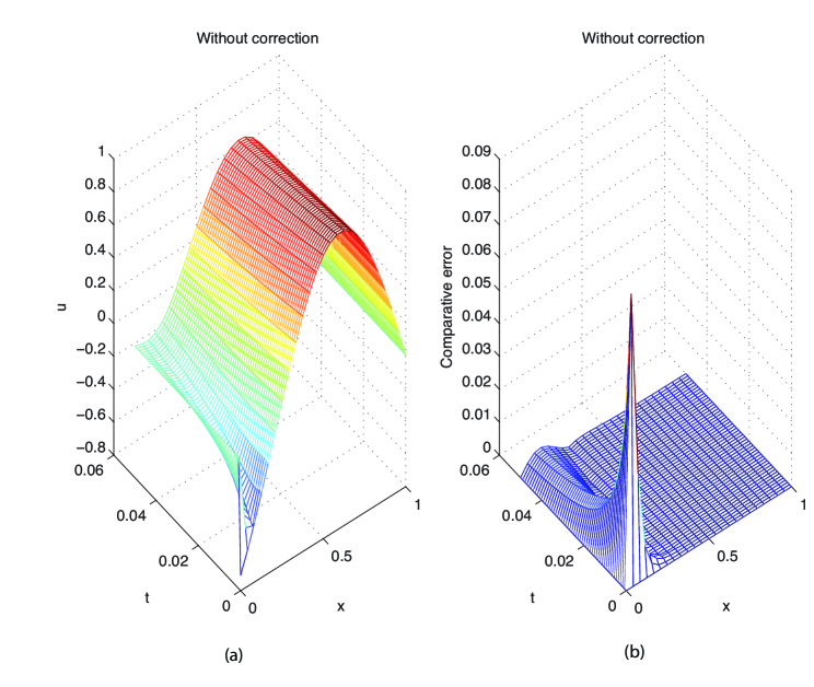
Figure 3.2: The solution, and pointwise errors without any correction procedure.

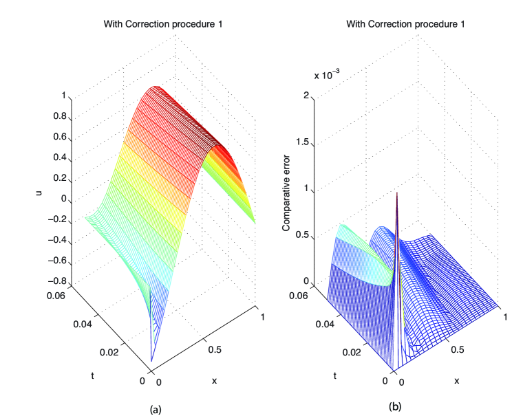
Figure 3.3: The solution, and pointwise errors with Correction procedure 1 applied.

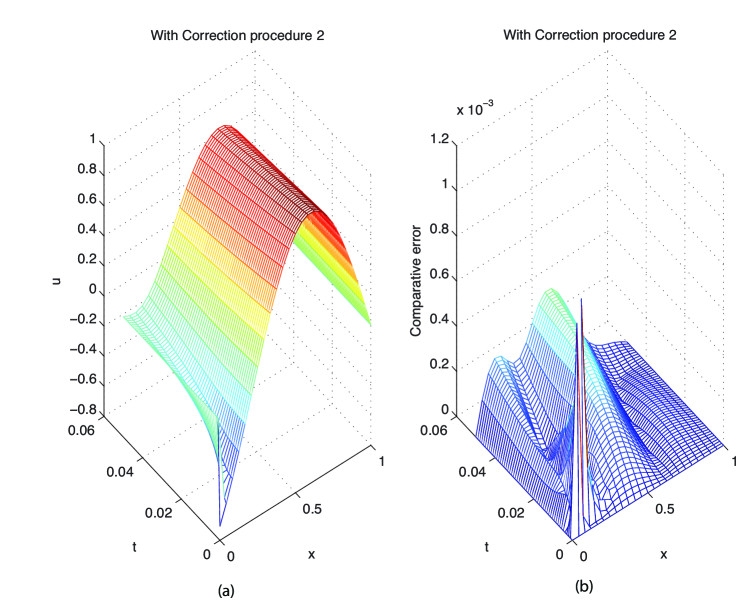
Figure 3.4: The solution, and pointwise errors with Correction procedure 2 applied.

The evolution of the maximum errors at each time step is plotted in Fig. 3.5 (a). The evolution of the maximum errors, with Correction Procedure 1 enabled, is displayed in Fig. 3.5 (b). The magnitude of the maximum errors has been reduced by roughly two orders (compared to Fig. 3.5 (a)).

When Correction Procedure 2 is enabled, we see further improvement in the accuracy, though it is less dramatic. For comparison we plot the result in the same figure as that for the result with Correction Procedure 1, and we see that the magnitude of the maximum errors is roughly halved.

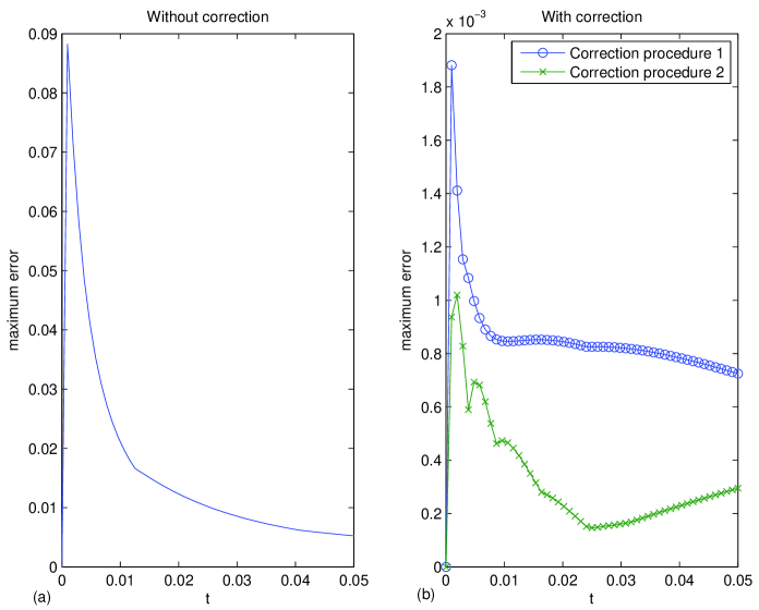
Figure 3.5: Evolution of the maximum errors till $t=0.05$. (a) Without correction procedure. (b) With correction procedure 1 and 2.

Remark 3.1.

In practice a correction procedure should be enabled during a short period of time at the beginning, and be disabled afterwards, when the solution has become smooth enough, to avoid the computational burden associated with the singular terms in (3.3). For computations that produced Fig. 3.5, however, we run the simulation for a short initial period of time only, and enable the correction procedure for the whole process to avoid unnecessary complications in programming.

Remark 3.2.

The zone of rapid variation of the solution and of the error should not be confused with a boundary layer effect. Indeed, firstly $\nu=0.2$ is too large to produce a sharp boundary layer, as the boundary layer size is of order $\sqrt{\nu}=0.447$ which is essentially of order 1. Furthermore when $\nu$ is small enough to produce a sharp boundary layer, it usually appears for all times, at either or both ends of the interval, $x=0,1$, whereas in our example the zone of rapid variation is concentrated near $x=0$, for a short time. Regarding the boundary layers for Burgers equation, see e.g. [1, 18], and also [5]. We intend to address in a future work the issue of the incompatible data as a boundary layer at time $t=0$; see as already a first result in this direction in [4].

3.3 Comparison of convergence rates

In this subsection we study the decay of the maximum errors, with and without the correction procedures applied. The results also demonstrate the effectiveness of the correction procedures.

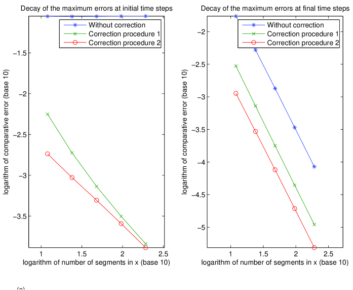
Figure 3.6: Decay of the maximum errors, (a) at the initial time step , (b) at final time step ($t=0.05$).

Fig. 3.6 (b) shows that, with and without the correction procedure applied, the maximum errors at a fixed time $t=0.05$ decay at approximately the second order (the slope of the line), which is the order of accuracy of the finite element scheme. However, the maximum errors of the simulation with Correction Procedure 1 applied is at a magnitude about one order smaller than without any correction procedure. The maximum errors of the simulation with Correction Procedure 2 applied is smaller by another magnitude of about $0.3$.

The most interesting and informative comparison can be made between the decay rates of the maximum errors at the initial time step ($t=\Delta t$, $\Delta t$ varying with different configurations). In Fig. 3.6 (a), the curve for the simulation without any correction procedure stick to the upper frame of the figure; the maximum errors wont come down whatsoever. With Correction procedure 1, the maximum errors decay at roughly the first order with respect to $\Delta x$, and with Correction procedure 2, the results are slightly better in terms of magnitude of the maximum errors.

4 A nonlinear reaction-diffusion equation

In this section we extend the previous correction procedures to the nonlinear reaction-diffusion equation:

$$\left\{\begin{aligned} &u_{t}-\nu u_{xx}+p(u)=0,0<x<1,t>0,\\ &u(0,t)=g_{1}(t),u(1,t)=g_{2}(t),t>0,\\ &u(x,0)=h(x),\end{aligned}\right.$$ (4.1)

where $\nu>0$ is a parameter representing viscosity; $g_{1}(t),g_{2}(t)$ and $h(x)$ are given functions; and $p(u)$ is a polynomial in $u$ of odd order and with a positive leading coefficient. The effectiveness of these correction procedures will be demonstrated by numerical results.

We first derive the compatibility conditions between the initial and boundary conditions of (4.1), as explained in Section 2.1:

$$0^{th}order:\hskip 11.38092pt\qquad g_{1}(0)=h(0),\qquad\qquad\qquad\hskip 5.97527ptg_{2}(0)=h(1),$$ (4.2)

$$1^{st}order:g_{1t}(0)=\nu h^{\prime\prime}(0)-p(h(0)),\quad g_{2t}(0)=\nu h^{\prime\prime}(1)-p(h(1)).$$ (4.3)

For simplicity, in what follows, we only consider the case where incompatibilities are present only at the left corner. Thus we let

$$\alpha_{0}\equiv g_{1}(0)-h(0)\neq 0,$$ (4.4)

$$\alpha_{1}\equiv g_{1t}(0)-\nu h^{\prime\prime}(0)+p(h(0))\neq 0.$$ (4.5)

$$\cdots\cdots\qquad\cdots\cdots$$ (4.6)

Of course the method we present for deriving the correction procedures would also apply to the incompatibilities at the right corner.

4.1 The correction procedure

As we did for the nonlinear convection–diffusion equation in Section 2 and 3, we shall combine the correction procedures with the weak formulation of $(\ref{e3.1})_{1}$, for the reason stated in Section 2.2. We multiply $(\ref{e3.1})_{1}$ by $v\in\mathfrak{D}(0,1)$ and integrate by parts to obtain the weak formulation of the equation:

$$(u_{t},v)+\nu(u_{x},v_{x})+(p(u),v)=0.$$ (4.7)

We intend to present the correction procedures (corrections of the incompatibilities to various order) in a unified way. To this end we shall employ the following notation:

$$S=\left\{\begin{aligned} &0&&\textrm{ if no correction procedure is applied},\\ &\alpha_{0}S_{0}&&\textrm{ if Correction procedure 1 is applied},\\ &\alpha_{0}S_{0}+\alpha_{1}S_{1}&&\textrm{ if Correction procedure 2 is applied}.\end{aligned}\right.$$ (4.8)

Here the singular corner functions $S_{0}$ and $S_{1}$ are defined as in (2.3) and (2.11) respectively. We let N be the number of segments in the interval $[0,1],h=1/N$ and let $V_{h}$ be the finite element space spanned by $(\varphi_{0},\varphi_{1},\cdots,\varphi_{N})$ (see Fig.1).

We look for the solutions of (4.7) in the form

$$u\simeq S+v_{h}(x,t),$$ (4.9)

where $v_{h}(\cdot,t)\in V_{h}$ for a.e. $t$. Plugging (4.9) into (4.7), and taking $v=\widetilde{v_{h}}\in V_{h}$ with $\widetilde{v}_{h}(0)=\widetilde{v}_{h}(1)=0$, we obtain

$$(v_{ht},\widetilde{v}_{h})+\nu(v_{hx},\widetilde{v}_{hx})+(p(v_{h}+S),\widetilde{v}_{h})=0.$$ (4.10)

Imposing the boundary conditions and initial conditions in (4.1) we have

$$\left\{\begin{aligned} &v_{h}(0,t)=g_{1}(t)-S(0,t),\\ &v_{h}(1,t)=g_{2}(t)-S(1,t),\end{aligned}\right.$$ (4.11)

and

$$v_{h}(x,0)=h(x).$$ (4.12)

We will solve (4.10), (4.11) and (4.12) for $v_{h}$, and then we recover $u$ by (4.9).

Concerning the compatibility conditions for $v_{h}$ we make the following observations. For the zeroth order correction procedure, $S=\alpha_{0}S_{0}$, and by (4.11) and (2.4), we have

$$\left\{\begin{aligned} &v_{h}(0,t)=g_{1}(t)-\alpha_{0},\\ &v_{h}(1,t)=g_{2}(t)-\alpha_{0}S_{0}(1,t).\end{aligned}\right.$$ (4.13)

The initial and boundary conditions for $v_{h}$ satisfy the zeroth order compatibility condition. Indeed,

$$g_{1}(0)-\alpha_{0}=h(0)$$ (4.14)

The compatibility conditions at the right corner are not affected.

For the first order correction procedure $S=\alpha_{0}S_{0}+\alpha_{1}S_{1}$, and by (4.11), (2.4) and (2.12),

$$\left\{\begin{aligned} &v_{h}(0,t)=g_{1}(t)-\alpha_{0}-\alpha_{1}t,\\ &v_{h}(1,t)=g_{2}(t)-\alpha_{0}S_{0}(1,t)-\alpha_{1}S_{1}(1,t).\end{aligned}\right.$$ (4.15)

It is easy to see that the initial and boundary condition for $v_{h}$ satisfy the zeroth order compatibility conditions. They also satisfy the first order compatibility condition. To see this, we insert (4.9) into $(\ref{e3.1})_{1}$ and obtain

$$v_{ht}-\nu v_{hxx}+p(\alpha_{0}S_{0}+\alpha_{1}S_{1}+v_{h})=0.$$ (4.16)

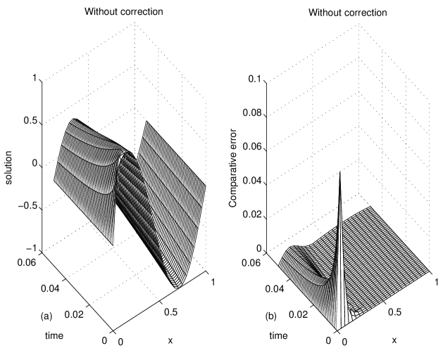
Figure 4.1: The solution, and pointwise errors without any correction procedure for $p(u)=u^{3}$.

We first calculate $v_{ht}(0,0)$ from(4.15):

$$v_{ht}(0,0)=g_{1t}(0)-\alpha_{1}$$ (4.17)

Then we calculate the same quantity from (4.16), using the initial condition (4.12) instead:

$$v_{ht}(0,0)=\nu h_{xx}(0)-p(h(0)).$$ (4.18)

The right-hand sides of (4.17) and (4.18) are equal according to (4.5)

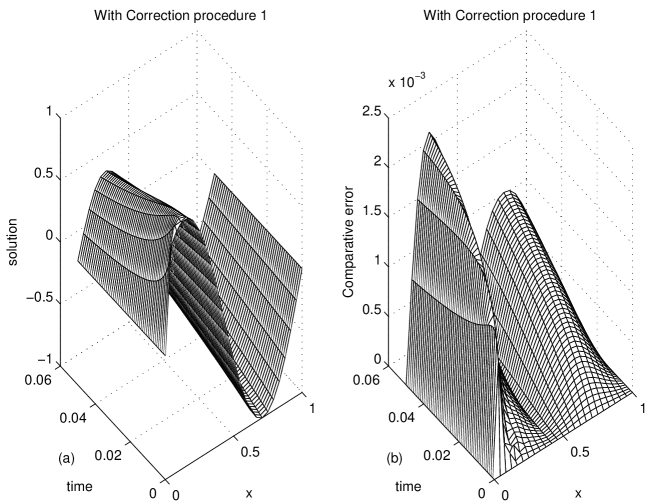
Figure 4.2: The solution, and the pointwise errors with Correction procedure 1 applied

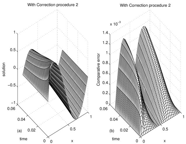
Figure 4.3: The solution, and the pointwise errors with Correction procedure 2 applied

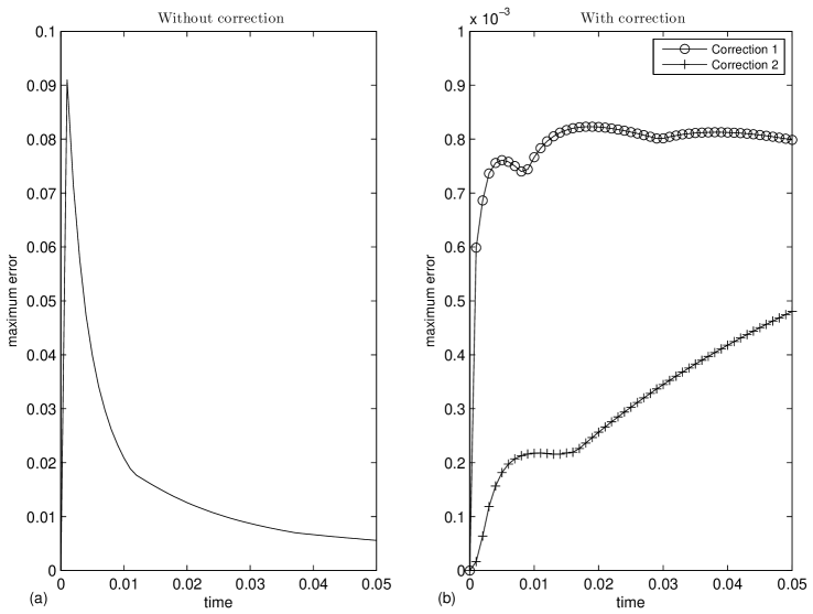
Figure 4.4: The evolution of the maximum errors till $t=0.05$: (a) without correction; (b) with Correction procedures 1 and 2.

4.2 The numerical results and interpretation

In the above we presented the correction procedures for reaction-diffusion equation with polynomial reaction terms. For the numerical testing of these correction procedures we consider the specific case where

$$p(u)=u^{3}.$$ (4.19)

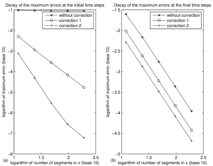
Figure 4.5: Decay of the maximum errors. (a) at initial step.(b)at final step.

As in Section 3.2, we take $\nu=0.2,\quad g_{1}=0,\quad g_{2}=0$ and $h=\sin(\frac{7\pi}{4}x+\frac{1}{4}\pi)$. It is easy to check that, for this test case, both the zeroth and the first order compatibility conditions at the right corner are met, but neither of them are met at the left corner.

Generally, given arbitrary initial and boundary conditions, it is impossible to find an analytic solution for the nonlinear reaction-diffusion equation. Therefore, in general, it is impossible to compute the real errors. As an alternative, we compute the comparative errors, which are the differences between the two numerical solutions for the problem, one with the mesh under consideration, and the other one with a finer mesh. In the following the term error is to be understood in this sense.
We first compute the solution of (4.1) without any correction procedure, i.e. with $S=0$ in (4.15). The solution is plotted in Fig. 4.1 (a), and it displays a sharp gradient around the left corner of the time–space axes due to the incompatibility between the initial and boundary conditions there. In order to have an overview of the structure of the errors in the solution we plot the pointwise errors in Fig. 4.1 (b). The pike appears near the left corner of the time–space axes, as expected, and it dissipates away quickly. For comparison we plot, in Fig. 4.2, the solution and the pointwise errors computed with Correction Procedure 1, and in Fig. 4.3, the solution and the pointwise errors computed with Correction Procedure 2. With Correction procedure 1 the magnitude of the errors at the left corner (see Fig. 4.2 (b)) has been reduced by roughly two orders (compared to Fig. 4.1 (b))! The most pronounced errors actually appear later in the simulation due to accumulation of the errors. With Correction procedure 2 the errors (Fig. 4.3) are further reduced by roughly one half (compared to Fig. 4.2).

The evolution of the maximum errors at each time step is plotted in Fig. 4.4 (a). The evolution of the maximum errors, with Correction Procedure 1 enabled, is displayed in Fig. 4.4 (b). The magnitude of the maximum errors has been reduced by indeed two orders (compared to Fig. 4.4 (a)).

When Correction Procedure 2 is enabled, we see further improvement in the accuracy, though it is less dramatic. For comparison we plot the result in the same figure (Fig. 4.4 (b)) as that for the result with Correction Procedure 1, and we see that the magnitude of the maximum errors is roughly halved.

4.3 Comparison of the convergence rates

In this subsection we study the decay of the maximum errors as functions of the mesh size(number of the segments in $x$), with and without the correction procedures applied. The results confirm the effectiveness of the correction procedures. Fig. 4.5 (b) shows that, with and without the correction procedure applied, the maximum errors at a fixed time $t=0.05$ decay at approximately the second order (the slope of the line), which is the order of accuracy of the finite element scheme. However, the maximum errors of the simulation when Correction procedure 1 is applied is about one half order smaller in magnitude than without any correction procedure. The maximum errors of the simulation with Correction procedure 2 applied is smaller by an additional factor of about $0.25$.

The most interesting and informative comparison can be made between the decay rates of the maximum errors at the initial time step ($t=\Delta t$, $\Delta t$ varying with different configurations). In Fig. 4.5 (a), the curve for the simulation without any correction procedure stick to the upper frame of the figure; the maximum errors will not come down whatsoever. With Correction procedure 1, the maximum errors decay at roughly the first order with respect to $\Delta x$, and with Correction procedure 2, the results are slightly better in terms of both the magnitude of the maximum errors and the decay rate.

5 Conclusion

Incompatibilities between the initial and boundary conditions for evolution PDEs have an adverse effect on the accuracy of numerical simulations, especially near the time–space corners. No matter how fine the grid is, the magnitude of the maximum errors persists, with the pike of the errors moving towards the corners as the grid gets finer.

For the same configuration, Correction procedure 1 reduces the magnitude of the maximum errors by about two orders; and Correction procedure 2 further reduces the magnitude by roughly one half.

For a fixed time, the correction procedures have no effect on the convergence rate of the solution at that point, but the correction procedures always give more accurate results, with Correction procedure 2 being more effective than Correction procedure 1. At the initial time step ($t=\Delta t$), without any correction procedure the magnitude of the maximum errors persists as mesh size gets small; with Correction procedures 1 or 2, the errors diminish at roughly order 1 with respect to $\Delta x$, with Correction procedure 2 doing slightly better than Correction procedure 1.

The approach described in this article for deriving correction procedures does not depend on any particular property of the viscous Burgers equation or the reaction–diffusion equation other than its diffusiveness. Hence we believe that these procedures can also be applied to other nonlinear diffusive equations in space dimension one. As mentioned earlier, in a work in progress [4] we study a totally different method related for higher space dimensions.

References

- [1] S. Akella and I. M. Navon, A comparative study of the performance of high resolution advection schemes in the context of data assimilation, Int. J. Numer. Meth. Fluids (2000).
- [2] L.K. Bieniasz, A singularity correction procedure for digital simulation of potential-step chronoamperometric transients in one–dimensional homogeneous reaction-diffusion systems, Electrochimica Acta 50 (2005), 3253–3261.
- [3] John P. Boyd and Natasha Flyer, Compatibility conditions for time-dependent partial differential equations and the rate of convergence of Chebyshev and Fourier spectral methods, Comput. Methods Appl. Mech. Engrg. 175 (1999), no. 3-4, 281–309. MR MR1702205 (2000d:65183)
- [4] Qingshan Chen, Zhen Qin, and Roger Temam, Numerical preparation of initial data, as to appear.
- [5] Haecheon Choi, Roger Temam, Parviz Moin, and John Kim, Feedback control for unsteady flow and its application to the stochastic burgers equation, J.Fluid Mech. 253 (1993), 509–543.
- [6] Natasha Flyer and Bengt Fornberg, Accurate numerical resolution of transients in initial-boundary value problems for the heat equation, J. Comput. Phys. 184 (2003), no. 2, 526–539. MR MR1959406 (2003m:65154)
- [7] , On the nature of initial-boundary value solutions for dispersive equations, SIAM J. Appl. Math. 64 (2003/04), no. 2, 546–564 (electronic). MR MR2049663 (2005a:35006)
- [8] Natasha Flyer and Paul N. Swarztrauber, The convergence of spectral and finite difference methods for initial-boundary value problems, SIAM J. Sci. Comput. 23 (2002), no. 5, 1731–1751 (electronic). MR MR1885081 (2002k:65122)
- [9] Avner Friedman, Partial differential equations of parabolic type, Prentice-Hall Inc., Englewood Cliffs, N.J., 1964. MR MR0181836 (31 #6062)
- [10] O. A. Ladyženskaja, V. A. Solonnikov, and N. N. Ural′ceva, Linear and quasilinear equations of parabolic type, Translated from the Russian by S. Smith. Translations of Mathematical Monographs, Vol. 23, American Mathematical Society, Providence, R.I., 1968. MR MR0241822 (39 #3159b)
- [11] O. Ladyženskaya, On the convergence of Fourier series defining a solution of a mixed problem for hyperbolic equations, Doklady Akad. Nauk SSSR (N.S.) 85 (1952), 481–484 (Russian). MR MR0051412 (14,474g)
- [12] O. A. Ladyženskaya, On solvability of the fundamental boundary problems for equations of parabolic and hyperbolic type, Dokl. Akad. Nauk SSSR (N.S.) 97 (1954), 395–398. MR MR0073834 (17,495c)
- [13] Jeffrey B. Rauch and Frank J. Massey, III, Differentiability of solutions to hyperbolic initial-boundary value problems, Trans. Amer. Math. Soc. 189 (1974), 303–318. MR MR0340832 (49 #5582)
- [14] Stephen Smale, Smooth solutions of the heat and wave equations, Comment. Math. Helv. 55 (1980), no. 1, 1–12. MR MR569242 (83d:35063)
- [15] R. Temam, Behaviour at time of the solutions of semilinear evolution equations, J. Differential Equations 43 (1982), no. 1, 73–92. MR 83c:35058
- [16] , Navier-Stokes equations, AMS Chelsea Publishing, Providence, RI, 2001, Theory and numerical analysis, Reprint of the 1984 edition. MR MR1846644 (2002j:76001)
- [17] Roger Temam, Suitable initial conditions, J. Comput. Phys. 218 (2006), no. 2, 443–450. MR MR2269371 (2007g:35077)
- [18] D. S. Zhang, G. W. Wei, and D. J. Kouri, Burgers equation with high reynolds number, Phys. Fluids 9 (1997), no. 6.