Fields Annihilation and Particles Creation in DBI inflation

Abstract

We consider a model of DBI inflation where two stacks of mobile branes are moving ultra relativistically in a warped throat. The stack closer to the tip of the throat is annihilated with the background anti-branes while inflation proceeds by the second stack. The effects of branes annihilation and particles creation during DBI inflation on the curvature perturbations power spectrum and the scalar spectral index are studied. We show that for super-horizon scales, modes which are outside the sound horizon at the time of branes collision, the spectral index has a shift to blue spectrum compared to the standard DBI inflation. For small scales the power spectrum approaches to its background DBI inflation value with the decaying superimposed oscillatory modulations.

I Introduction

Inflation proved to be very successful as a theory of early universe and structure formation Guth:1980zm which is strongly supported by cosmic observations Komatsu:2010fb . The simplest models of inflation are based on a scalar field minimally coupled to gravity with a potential flat enough to support an extended period of inflation. Despite its observational successes there is no deep theoretical understanding of inflation and the nature of the inflation field. There have been many attempts during past decade to embed inflation within the context of string theory, for a review see HenryTye:2006uv ; Cline:2006hu ; Burgess:2007pz ; McAllister:2007bg ; Baumann:2009ni ; Mazumdar:2010sa and references therein.

Brane inflation is an interesting realization of inflation from string theory dvali-tye ; Alexander:2001ks ; collection ; Dvali:2001fw . In its original form, it contained a pair of D3 and anti D3 branes moving in the Calabi-Yau (CY) compactification. The inflaton field is the radial distance between them so in this sense the inflaton field has a geometric interpretation in string theory. Inflation ends when the distance between the brane and the anti-brane reaches the string length scale where a tachyon develops in the open strings spectrum stretched between the pair. Inflation ends soon after tachyon formation and the energy stored in branes tensions are released into closed string modes HenryTye:2006uv . However, it was soon realized that the potential between the pair of brane and anti-brane is too steep to allow a long enough period of slow-roll inflation. To flatten the potential, it was suggested to put the pair of brane and anti-brane inside a warped throat Klebanov:2000hb ; Giddings:2001yu ; Dasgupta:1999ss , where the potential between D3 and $\overline{\mbox{D3}}$ is warped down as in Randall-Sundrum scenario Randall:1999ee ; Kachru:2003sx ; Firouzjahi:2003zy ; Burgess:2004kv ; Buchel ; Iizuka:2004ct ; Firouzjahi:2005dh ; Baumann:2006th ; Burgess:2006cb ; Baumann:2007ah ; Chen:2008au ; Cline:2009pu .

As a novel feature of brane inflation the question of branes annihilation and particles creation during inflation was studied in Battefeld:2010rf . In this picture two stacks of branes, located at different places inside the throat, are moving in the slow-roll limit towards the bottom of the throat where anti-branes are located. The stack closer to the tip will be annihilated during inflation transferring its energy into closed string modes. The second stage of inflation is driven by the remaining stack of branes until it is annihilated by the remaining anti-branes at the bottom of the throat. The process of fields annihilation Battefeld:2008py ; Battefeld:2008ur and particle creations Barnaby:2009mc ; Barnaby:2009dd ; Barnaby:2010ke ; Barnaby:2010sq ; Green:2009ds ; Brax:2010tq ; Cai:2010wt can have interesting observational consequences on CMB. Here we generalize the results in Battefeld:2010rf to the case where the mobile stacks of branes are moving ultra relativistically as in DBI inflation Alishahiha:2004eh . As in Battefeld:2010rf , the stack closer to the tip is annihilated by the background anti-branes resulting in particles creation during inflation while the second stage of inflation is driven by the remaining stack.

The rest of the paper is organized as follows. In section II we present our set up and background solutions for DBI inflation. In section III we study the curvature perturbations and present our matching conditions. In section IV we obtain the power spectrum of curvature perturbations and the spectral index. Discussions and conclusions are presented in section V.

II The model and background equations

In this section we present our set up. As explained above we consider two stacks containing $p_{1}$ and $p_{2}$ coincident branes. The positions of the stacks are represented by functions $r_{1}(t)$ and $r_{2}(t)$ inside the throat. There are $p_{1}+p_{2}$ anti-branes located at the bottom of the throat, $r_{0}$. We assume that the first stack is closer to the tip of the throat so it is annihilated during inflation transferring its energy into closed strings modes. The second stage of inflation is driven by the remaining stack of $p_{2}$ branes. For a schematic view, see Fig. 1 and Fig. 2.

Figure 1: A schematic view of the set up. There are two stacks containing $p_{1}$ and $p_{2}$ coincident branes inside the throat. The stacks are moving relativistically towards the bottom of the throat where there are $p_{1}+p_{2}$ anti-branes. The figure is borrowed from Battefeld:2010rf

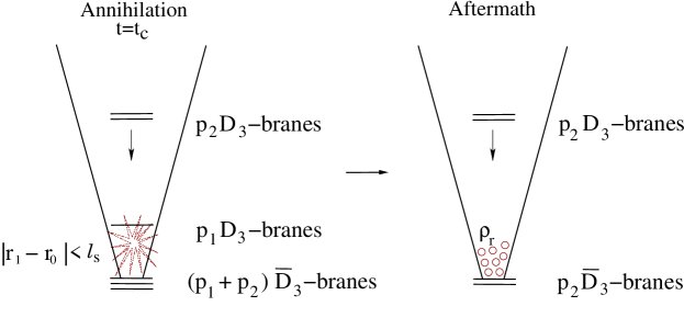
Figure 2: A schematic view of the annihilation event at $t_{c}$. The stack closer to the tip of the throat is annihilated during inflation transferring its energy into radiation. The second stage of inflation is driven by the remaining stack containing $p_{2}$ branes. Inflation ends when this stack is annihilated by the remaining $p_{2}$ anti-branes at the bottom of the throat. The figure is borrowed from Battefeld:2010rf .

As usual the metric of the throat is

$$ds^{2}=h^{-\frac{1}{2}}(r)g_{\mu\nu}dx^{\mu}dx^{\nu}+h^{\frac{1}{2}}(r)(dr^{2}+r^{2}d\Omega_{5}^{2})\,,$$ (1)

where $r$ is the radial coordinate, $d\Omega_{5}^{2}$ represents the internal five-dimensional azimuthal directions which we may take to be an $S^{5}$ and $h(r)$ is the warp factor

$$h(r)=\frac{L^{4}}{r^{4}}\,.$$ (2)

Here $L$ is the AdS length scale of the throat which is created by $N$ coincident background branes located at $r=0$ (for a review see Herzog:2001xk ),

$$L^{4}=4\pi g_{s}N\alpha^{\prime 2}\,,$$ (3)

where $g_{s}$ is the perturbative string coupling and $\alpha^{\prime}=l_{s}^{2}$ where $l_{s}$ is the string length scale. The mobile stacks of $p_{1}$ and $p_{2}$ branes are located at positions $r_{1}$ and $r_{2}$ as probe branes. In order for our probe branes approximation to be valid, we need $p_{1},p_{2}\ll N$. In addition there are $p_{1}+p_{2}$ $\overline{\mbox{D3}}$ branes at the bottom of the throat $r_{0}$. Once the distance between the stack of $p_{1}$ branes and these anti-branes reaches at the order of $l_{s}$ the open strings stretched between them become tachyonic, indicating an instability in the system. Shortly after tachyon formation, the stack of $p_{1}$ branes is annihilated by $p_{1}$ anti-branes at the bottom of the throat. Consequently, the energy stored in $p_{1}$ branes and anti-branes tension, which is $2p_{1}T_{3}h(r_{0})^{-2}$, is transferred into closed strings modes. For simplicity, we assume that these closed strings modes are in the form of massless particles (radiation). Of course a combinations of massive and massless particles would be created. However, once these particles are created they will be diluted quickly by the background inflation so for our practical purposes, there are not much differences between massive and massless particle creations.

The goal of this work is to examine the effects of branes annihilation and particles creation on the remaining field which drives the second stage of inflation. In Battefeld:2010rf this was studied for the case where the stacks are moving slowly. Here we generalize those analysis to our case at hand where the stacks are moving ultra relativistically Alishahiha:2004eh ; Chen:2004gc ; Shandera:2006ax ; Bean:2007eh ; Bean:2007hc ; Chen:2006nt .

The Dirac-Born-Infeld (DBI) action for the stacks of $p_{1}$ and $p_{2}$ branes moving relativistically in the background of Eq. (1) is

$$S=\sum_{I=1}^{2}p_{I}T_{3}\int\sqrt{-g}\,d^{4}x\left[h^{-1}(r_{I})\left(1-\sqrt{1-h(r_{I})\,{\dot{r}_{I}}^{2}}\right)-V_{I}(r_{I})\right]\,,$$ (4)

where $T_{3}$ is the D3-brane tension with $T_{3}L^{4}=\frac{N}{2\pi^{2}}$. We also have added the unknown contributions $V_{1}(r_{1})$ and $V_{2}(r_{2})$ from the back-reactions of the background fluxes, branes and Kahler modulus stabilization on the dynamics of mobile branes Kachru:2003sx ; Firouzjahi:2005dh . As usual, we shall continue from the phenomenological point of views and parametrize these potentials to be suitable for inflation Alishahiha:2004eh ; Chen:2004gc ; Shandera:2006ax ; Bean:2007eh ; Bean:2007hc ; Chen:2006nt ; Thomas:2007sj ; Huston:2008ku .

To proceed further, we simplify the DBI action into the following form which is more suitable for our analysis

$$S=\sum_{I=1}^{2}\int d^{4}x\sqrt{-g}\left[f_{I}^{-1}\left(1-\sqrt{1-f_{I}{\dot{\phi}_{I}}^{2}}\right)-V_{I}(\phi_{I})\right]\,,$$ (5)

where $\phi_{I}\equiv\sqrt{T_{3}p_{I}}r_{I}$, $f_{I}\equiv\frac{\lambda_{I}}{\phi_{I}^{4}}$ and $\lambda_{I}\equiv T_{3}L^{4}p_{I}=\frac{Np_{I}}{2\pi^{2}}$. This form of multiple field DBI inflation has been studied extensively in the past Cai:2008if .

Now we are ready to promote the system into a cosmological set up. The background four-dimensional FRW metric is

$$ds^{2}=-dt^{2}+a(t)^{2}d\vec{x}^{2}\,,$$ (6)

where $a(t)$ is the scale factor. The Friedmann equation and the energy conservation equations are

$$3H^{2}=\frac{\rho}{M^{2}_{p}}\quad\quad,\quad\quad\dot{\rho}+3H(\rho+P)=0\,,$$ (7)

where $H=\dot{a}/a$ is the Hubble expansion rate. The energy density $\rho$ and the pressure $p$ are given by

$$\rho=\sum_{I}\left[f_{I}^{-1}(\gamma_{I}-1)+V_{I}\right]\quad\quad,\quad\quad p=\sum_{I}\left[f_{I}^{-1}(1-\gamma_{I}^{-1})-V_{I}\right]\,.$$ (8)

Here the Lorentz factor for each field, $\gamma_{I}$, is defined by

$$\gamma_{I}=\frac{1}{\sqrt{1-f_{I}\dot{\phi}_{I}^{2}}}\,.$$ (9)

Finally, the background Klein-Gordon equation for each field is

$$\ddot{\phi}_{I}+3H\gamma_{I}^{-2}\dot{\phi}_{I}+\frac{3}{2}\frac{{f^{\prime}_{I}}}{f_{I}}\dot{\phi}_{I}^{2}-\frac{{f^{\prime}_{I}}}{f_{I}^{2}}+\gamma_{I}^{-3}\left({V_{I}^{\prime}}+\frac{{f^{\prime}_{I}}}{f_{I}^{2}}\right)=0\,.$$ (10)

So far we have not specified the form of the potentials, $V_{I}(\phi_{I})$. As explained above, these potentials arise from the back-reactions of the fluxes, branes and Kahler modulus stabilization to the mobile branes. It is a non-trivial question in string theory as how one can calculate these back-reactions Baumann:2006th ; Burgess:2006cb ; Chen:2008au concretely. However, to be specific, we consider the phenomenological approach where the potentials have the form $V_{I}=\frac{m_{I}^{2}}{2}\phi_{I}^{2}$. We shall also keep the masses $m_{I}$ undetermined except that their magnitudes should be such that they give the desired number of e-foldings and fit the CMB observations such as the COBE normalization.

We are interested in the limit where the branes are moving ultra relativistically inside the throat so one can not expand the square root in Eq. (5) perturbatively in terms of $\dot{\phi}$. This corresponds to the case where $\gamma\gg 1$ and the stacks of branes are approaching the speed limit $\dot{\phi}_{I}^{2}\simeq f_{I}^{-1}$. In this limit Eq. (10) reduces to

$$\ddot{\phi}_{I}+\frac{3}{2}\frac{{f^{\prime}_{I}}}{f_{I}}\dot{\phi}_{I}^{2}-\frac{{f^{\prime}_{I}}}{f_{I}^{2}}=0\,,$$ (11)

which can be verified to have the speed limit solution $\phi_{I}(t)\simeq\frac{\sqrt{\lambda}_{I}}{t}$. One can plug this solution back into Eq. (10) to find the next leading correction and

$$\phi_{I}(t)\simeq\frac{\sqrt{\lambda}_{I}}{t}\left(1-\frac{9H^{2}}{2m_{I}^{4}\,t^{2}}\right)\,.$$ (12)

To get this solution, we have neglected the variation of $H$ during inflation to leading order.

To obtain the solution for the scale factor $a(t)$ we require that the energy density is dominated by the potential energy so the Friedmann equation (7) reduces to $\dot{a}/a\propto 1/t$. Below we find the background solutions for both inflationary stages, before the collision and after the collision.

II.0.1 Before Collision

Before collision both stacks contribute to the energy density and the Friedmann equation can easily be solved to give

$$\frac{\dot{a}}{a}=\frac{{\Lambda_{-}}}{t}\,,$$ (13)

where the dimensionless number $\Lambda_{-}$ is defined by

$$\Lambda_{-}\equiv\left(\sum_{i}\frac{\lambda_{i}m_{i}^{2}}{6M_{p}^{2}}\right)^{1/2}\,.$$ (14)

Working with the number of e-foldings $N(t)$ as the clock, $dN=Hdt$, one obtains

$$N(t)=\Lambda_{-}\ln\frac{t}{t_{in}}\,,$$ (15)

where $t_{in}$ is the time at the start of inflation when $N=0$. Define $N=N_{c}$ the time when the first branes collision take place and the stack of $p_{1}$ branes is annihilated by $p_{1}$ background anti-branes. Similarly, define $\phi_{I}=\phi_{Ic}$ as the corresponding fields values at the time of collision. Combining Eqs. (15) and (12) yield

$$\phi_{Ic}\simeq\phi_{Iin}e^{-\frac{N_{c}}{\Lambda_{-}}}\,,$$ (16)

where $\phi_{Iin}$ are the corresponding fields values at the start of inflation.

One can find an approximate formula for the time of branes collision as follows. As mentioned before, the time of branes annihilation is when the physical distance between the stack of $p_{1}$ branes and anti-branes located at the bottom of the throat $r_{0}$ reaches the string length scale $l_{s}$. Starting with the metric (1) the physical distance between the first stack and the anti-branes, $\Delta\ell$, is calculated to be

$$\Delta\ell=\int_{r_{0}}^{r_{1}}h(r)^{1/4}dr=L\,\ln\frac{r_{1}}{r_{0}}\,.$$ (17)

Setting $\Delta\ell=l_{s}$ and using Eq. (16) the onset of branes collision, $N=N_{c}$, is obtained to be

$$N_{c} \simeq \Lambda_{-}\left(\ln\frac{\phi_{1in}}{\phi_{1A}}-\frac{l_{s}}{L}\right)$$ (18)

$$\simeq \Lambda_{-}\left(\ln\frac{\phi_{1in}}{\phi_{1A}}-(4\pi g_{s}N)^{-1/4}\right)\,,$$

where to get the final relation Eq. (3) has been used. Here we defined $\phi_{IA}\equiv\sqrt{p_{I}T_{3}}r_{0}$ as the values of the corresponding fields at the position of the anti-branes.

Correspondingly, the position of $\phi_{2}$ at the time of collision is obtained to be

$$\phi_{2c}\simeq\frac{\sqrt{\lambda_{2}}}{t_{c}}\simeq\phi_{2in}e^{-\frac{N_{c}}{\Lambda_{-}}}\,.$$ (19)

Also it is instructive to calculate $\gamma_{I}$. Using Eqs. (12) and (13) in the expression of $\gamma_{I}$ one finds

$$\gamma_{I}^{-}\simeq\frac{m_{I}^{2}\,t^{2}}{3{\Lambda_{-}}}\,.$$ (20)

This indicates that as inflation proceeds, $\gamma_{I}$ increases like $t^{2}$.

II.0.2 After Collision

After the first stack is annihilated, the second stage of inflation is driven by the remaining stack of $p_{2}$ branes and the scale factor is given by $\frac{\dot{a}}{a}=\frac{{\Lambda_{+}}}{t}$ where now

$$\Lambda_{+}\equiv\left(\frac{\lambda_{2}m_{2}^{2}}{6M_{P}^{2}}\right)^{1/2}\,.$$ (21)

Defining the total number of e-foldings by $N_{T}$, with $N_{T}\sim 60$ to solve the flatness and the horizon problem, one has

$$N_{T}-N_{c}\simeq{\Lambda_{+}}\ln\frac{t_{f}}{t_{c}}\,,$$ (22)

where $t_{f}$ is the time of end of inflation when the second stack is annihilated by the remaining $p_{2}$ anti-branes. As before, this happens when the physical distance between the second stack and the anti-branes reaches the string scale $l_{s}$ which can be used to determine the value of $\phi_{2}$ at the end of inflation $\phi_{2f}\simeq\phi_{2A}\exp(l_{s}/L)$. Similarly, one can show

$$N_{T} \simeq N_{c}+{\Lambda_{+}}\ln\frac{\phi_{2c}}{\phi_{2f}}$$ (23)

$$\simeq \left(1-{\frac{\Lambda_{+}}{\Lambda_{-}}}\right)N_{c}+{\Lambda_{+}}\ln\left[\frac{\phi_{2in}}{\phi_{2A}}-(4\pi g_{s}N)^{-1/4}\right]\,,$$

One should arrange the background parameters such as $g_{s}N$, $\Lambda_{\pm}$ and $\phi_{Iin}$ such that large enough $N_{T}$ can be obtained to solve the flatness and the horizon problem.

Correspondingly, the Lorentz factor after the collision is

$$\gamma_{2}^{+}\simeq\sqrt{\frac{2}{3}}\frac{m_{2}M_{P}t^{2}}{\sqrt{\lambda_{2}}}\,.$$ (24)

One can find a measure of the magnitudes of $\Lambda_{\pm}$ as follows. For DBI inflation to match the COBE normalization, one requires a large background charges such that $g_{s}N\gg 1$ Alishahiha:2004eh ; Baumann:2006cd so one can safely neglect this term in Eqs. (23) and (18). Assuming that there is not exponential hierarchy between $\phi_{2in}$ and $\phi_{2A}$ one concludes that ${\Lambda_{+}}\lesssim N_{T}$. However, by keeping the ratio $\frac{\phi_{2in}}{\phi_{2A}}$ exponentially large in the light of Giddings:2001yu , one can lower ${\Lambda_{+}}$ by a factor of ten or so. In our analysis below, we shall take take ${\Lambda_{+}}\simeq{\Lambda_{-}}\gg 1$.

As shown in Alishahiha:2004eh significant amount of non-Gaussianities can be created in DBI inflation where the branes are moving ultra-relativistically. The non-Gaussianity parameter $f_{NL}$ is related to the Lorentz factor via $f_{NL}\simeq-0.3\gamma^{2}$. To satisfy the WMAP constraints on $f_{NL}$ one requires that $\gamma<31$ Shandera:2006ax ; Bean:2007eh ; Bean:2007hc .

III Perturbations

Having studied our inflationary background in some details, now we consider the perturbations in this background. As discussed in Battefeld:2010rf a complete treatment of perturbations in our set up with branes annihilation and particles creation is a non-trivial task. The process of field annihilation and particles creation are determined by the dynamics of open string tachyon condensation. In the presence of background branes and fluxes this is a non-trivial phenomena Jones:2003ae ; Jones:2002sia . We shall instead take the phenomenological approach and impose some physically reasonable approximations to bypass these difficulties.

Before the collision we have two scalar fields $\phi_{1}$ and $\phi_{2}$ corresponding to two stacks of branes moving relativistically. After the collision, the energy associated with field $\phi_{1}$ is transferred into closed strings modes, which we approximate them as massless particles. The process of field annihilation and closed strings formation takes some time scale, $\Delta t$. In our set up where the collision happens at the bottom of the throat $\Delta t$ is given by the inverse of the warped string mass scale, that is $\Delta t\simeq h(r_{0})^{1/4}m_{s}^{-1}$ where $m_{s}=l_{s}^{-1}$ is the string theory mass scale. Note that the factor $h(r_{0})^{1/4}$ in $\Delta t$ is in the light of Randall-Sundrum idea Randall:1999ee . In our effective four-dimensional approach where $H\ll m_{s}$, we can take the process of field annihilation and particles creation as instantaneous and set $\Delta t\sim 0$ for practical purposes. This approximations is certainly true for large scale perturbations.

To be slightly more specific, we can borrow the results of Barnaby:2004gg ; Kofman:2005yz ; Firouzjahi:2005qs ; Chen:2006ni . As mentioned before, after brane and anti-brane annihilation their energy is transferred into closed strings modes. Subsequently, these modes cascade down to graviton zero mode and the Kaluza-Klein (KK) excitations. This happens in a time scale controlled by the inverse of the warped sting mass scale, much shorter than $H^{-1}$. Subsequently, the massive KK modes decay into lighter modes. Because of the warp factor, the wave function of these modes are highly peaked at the bottom of the throat where the annihilation takes place. Their effects on the remaining stack of $p_{2}$ branes at position $r_{2}$ may be negligible in the limit where the stack of $p_{2}$ branes is far away from the tip of the throat.

Even in the instantaneous brane annihilation approximation it is not clear within string theory set up as how to turn off field $\phi_{1}$ and turn on radiation. To bypass this shortcoming we follow the practical approach employed in Battefeld:2010rf . We assume that field $\phi_{1}$ is subdominant in the background energy density, corresponding to $V_{1}\ll V_{2}$. After $\phi_{1}$ is annihilated, we assume that not only its energy is transferred into radiation energy density, $\rho_{r}$, but also the perturbations carried by $\delta\phi_{1}$ are transferred into perturbations in radiation, $\delta\rho_{r}$. We also assume that the perturbations $\delta\rho_{r}$, before significantly diluted by the background expansion, do not interfere with $\delta\phi_{2}$ after collision. This can be considered as a higher order back-reaction, perhaps controlled by the ratio $p_{1}/p_{2}$, which we take to be small. Also this back-reaction may be negligible as long as the separation between two stacks of branes are large enough inside the throat. Within these approximations we do not need to follow the perturbations carried by $\delta\phi_{1}$ before the collision and the perturbations carried by $\delta\rho_{r}$ after the collision. In these approximations we shall follow only the perturbations $\delta\phi_{2}$ before and after the collision. This may not be such a bad approximation because physical quantities, such as curvature perturbations, are calculated at the end of inflation when only field $\phi_{2}$ and its perturbations are present. Since we do not follow $\delta\phi_{1}$ and $\delta\rho_{r}$, our treatments of perturbations eventually reduce to those of single field model where only $\delta\phi_{2}$ is counted before and after the branes collision. However, the effect of $\phi_{1}$ and radiation is kept in the background so that is how $\delta\phi_{2}$ feels their presences.

III.1 Perturbations Equations

With these approximations we start the analysis of perturbations in our set up. The metric perturbations in the conformal Newtonian gauge where there is no anisotropy in stress energy tensor is

$$ds^{2}=-(1+2\Phi)dt^{2}+(1-2\Phi)a^{2}(t)\delta_{ij}dx^{i}dx^{j}\,,$$ (25)

where $\Phi(t,x)$ is the Bardeen potential which in this gauge coincides with the Newtonian potential.

Defining the curvature perturbations ${\cal R}_{2}$ on comoving surface $\phi_{2}=constant$ via

$$\mathcal{R}_{2}\equiv H\frac{{\delta\phi}_{2}}{\dot{\phi_{I}}}+\Phi\,,$$ (26)

and introducing the Sasaki-Mukhanov variables $v_{2}$

$$v_{2}=z_{2}{\cal R}_{2}\quad,\quad z_{2}\equiv\frac{a\dot{\phi}_{2}\gamma_{2}^{3/2}}{H}\,,$$ (27)

one obtains the following standard second order differential equation Garriga:1999vw

$$v_{2}^{{}^{\prime\prime}}+\left(k^{2}c_{s}^{2}-\frac{z_{2}^{\prime\prime}}{z_{2}}\right)v_{2}=0\,.$$ (28)

Here the prime denotes the derivative with respect to the conformal time $d\tau=dt/a(t)$ and $c_{s}$ is the sound speed associated with $\phi_{2}$ perturbations defined by

$$c_{s}=\gamma_{2}^{-1}=\sqrt{1-f_{2}\dot{\phi}_{2}^{2}}\,.$$ (29)

As mentioned before, we work in the ultra relativistic limit where $\gamma_{I}\gg 1$ corresponding to a very small sound speed $c_{s}\ll 1$. This has interesting consequences for non-Gaussianities Alishahiha:2004eh ; Chen:2006nt .

To solve Eq. (28) we need to find the form of $z_{2}$. Plugging different components of $z_{2}$ from the background specified in the previous section, one obtains

$$z_{2}^{\pm}\propto t^{{\Lambda_{\pm}}+2}\propto\tau^{-\frac{{\Lambda_{\pm}}+2}{{\Lambda_{\pm}}-1}}\,.$$ (30)

This in turn yields

$$\frac{{z^{\prime\prime}_{2\pm}}}{z_{2\pm}}=\frac{2\Lambda_{\pm}^{2}+5{\Lambda_{\pm}}+2}{\left(\Lambda_{\pm}^{2}-2{\Lambda_{\pm}}+1\right)\tau^{2}}\simeq\left(2+\frac{9}{{\Lambda_{\pm}}}\right){\tau^{-2}}\,,$$ (31)

where to get the final approximation the relation ${\Lambda_{\pm}}\gg 1$ is used as explained in previous section. Consequently, one can cast Eq. (28) into more conventional form

$${v^{{}^{\prime\prime}}_{2}}_{\mp}+\left(k^{2}{c_{s}^{2}}-\frac{\mu_{\mp}^{2}-1/4}{\tau^{2}}\right){v_{2}}_{\mp}=0\,,$$ (32)

where the indices $\mu_{\pm}$ are given by

$$\mu_{\pm}\simeq\frac{3}{2}+\frac{3}{{\Lambda_{\pm}}}\equiv\frac{3}{2}+3\epsilon_{\pm}\,.$$ (33)

We have defined the “slow-roll” parameter $\epsilon_{\pm}\equiv\frac{-\dot{H}_{\pm}}{H_{\pm}}\simeq\frac{1}{\Lambda_{\pm}}$ for the later convenience. As argued before, $\epsilon_{\pm}\simeq 1/N_{T}\ll 1$.

One should solve Eq. (32) for both $t<t_{c}$ and $t>t_{c}$ and glue the solutions via the matching conditions. In the limit where we can neglect the running of $c_{s}$ the solutions of Eq. (32) as usual are given in terms of Hankel functions $H_{\mu_{\pm}}^{(1)}(-c_{s}k\tau)$ and $H_{\mu_{\pm}}^{(2)}(-c_{s}k\tau)$. At the early stage of inflation when all physically relevant modes are inside the sound horizon, corresponding to $-c_{s}k\tau\rightarrow\infty$, the solutions are given in terms of positive frequency modes $\frac{1}{\sqrt{2c_{s}k}}e^{-ic_{s}k\tau}$ created from vacuum. This initial condition eliminates $H_{\mu_{\pm}}^{(2)}(-c_{s}k\tau)$ and the solution of Eq. (32) during the first inflationary stage is

$${v_{2}}_{-}=\frac{\sqrt{-\pi\tau}}{2}e^{i\pi(\mu_{-}+1/2)/2}H^{(1)}_{\mu_{-}}(-c_{s}k\tau)\,.$$ (34)

After the collision, due to particles creation, the system is not in vacuum and both solutions $H_{\mu_{\pm}}^{(1)}(-c_{s}k\tau)$ and $H_{\mu_{\pm}}^{(2)}(-c_{s}k\tau)$ are permitted. We parametrize the solution after the collision in terms of the coefficients $\alpha$ and $\beta$ via

$${v_{2}}_{+}=\frac{\sqrt{-\pi\tau}}{2}e^{i\pi(\mu_{+}+1/2)/2}\left[\alpha H^{(1)}_{\mu_{+}}(-c_{s}k\tau)+\beta H^{(2)}_{\mu_{+}}(-c_{s}k\tau)\right]\,.$$ (35)

In the absence of any brane collision and particles creation $\alpha=1,\beta=0$, $\mu_{-}=\mu_{+}$ and the two solutions (34) and (35) coincides. Our job below is to find the coefficients $\alpha$ and $\beta$ and read off the final value of curvature perturbations as a function of $\alpha$ and $\beta$. For this purpose, we need to impose our matching prescriptions, joining Eqs. (34) and (35) at the time of collision $\tau=\tau_{c}$.

III.2 Matching Conditions

Imposing the matching condition is the most important step in our analysis of perturbations. There are standard prescriptions in literature for imposing the cosmological matching conditions in systems where there is a sudden jump in equation of state Deruelle:1995kd ; Martin:1997zd . More specifically, in models where the matching conditions are imposed on a comoving hyper-surface one requires that both the extrinsic and the intrinsic curvatures to be continuos across this hyper-surface. These result in the following matching conditions Zaballa:2009xb ; Lyth:2005ze ; Zaballa:2006kh

$$[\Phi]_{-}^{+}=[{\cal R}]_{-}^{+}=0\,,$$ (36)

where $\Phi$ is the gauge invariant Bardeen potential and ${\cal R}$ is the comoving curvature perturbations.

In principle we can also impose these matching conditions in our system. However, as mentioned at the start of this section, we do not have a theoretical control on the dynamics of tachyon condensation, fields annihilation and particles creation. These shortcomings in turn result in a lack of knowledge of $\Phi$ and ${\cal R}$ after the collision. To bypass these shortcomings we have chosen the phenomenological approach where only the perturbations of $\phi_{2}$ are followed before and after the collision. In this approximation our model is effectively a single field scenario with the extra modification that the effects of particles creation are kept at the background level. This in turn results in different indices for Hankel functions, $\mu_{-}\neq\mu_{+}$. In this view, our method is very similar to the method used in Joy:2007na where the effects of phase transitions in a multiple field model is translated into a sudden violation of slow-roll parameters in an effective single field model. Therefore in our studies here, as in Joy:2007na , one expects that the matching conditions (36) are simplified into

$$[v_{2}]_{-}^{+}=[v_{2}^{\prime}]_{-}^{+}=0\,,$$ (37)

i.e. both $v_{2}$ and $v_{2}^{\prime}$ are continuous across the surface of branes collision.

Using the matching conditions (37) in Eqs. (34) and (35) one obtains

$$\alpha = -\frac{i\pi x}{4}e^{i\delta}\left[H^{\prime(1)}_{\mu^{-}}(x)H^{(2)}_{\mu^{+}}(x)-H^{(1)}_{\mu^{-}}(x)H^{\prime(2)}_{\mu^{+}}(x)\right]$$

$$\beta = \frac{i\pi x}{4}e^{i\delta}\left[H^{\prime(1)}_{\mu^{-}}(x)H^{(1)}_{\mu^{+}}(x)-H^{(1)}_{\mu^{-}}(x)H^{\prime(1)}_{\mu^{+}}(x)\right]\,,$$ (38)

where the derivatives are with respect to the arguments of the Hankel functions and

$$x\equiv-c_{s}k\tau_{c}\quad,\quad\delta\equiv\frac{\pi}{2}(\mu_{-}-\mu_{+})\,.$$ (39)

IV Power Spectrum

We are in a position to calculate the curvature power spectrum ${\cal P}_{\cal R}$ at the end of inflation. The curvature power spectrum is defined via

$$\delta^{3}({\bf k}-{\bf k}^{\prime})\mathcal{P}_{\mathcal{R}}=\frac{4\pi k^{3}}{(2\pi)^{3}}\langle\mathcal{R}({\bf k}^{\prime})^{*}\mathcal{R}({\bf k})\rangle\,.$$ (40)

Since only the field $\phi_{2}$ is present at the end of inflation we only need the power spectrum of ${\cal R}_{2}$. Using Eqs. (26) and (27) one obtains

$${\cal R}_{2}=\frac{Hv_{2}}{a\dot{\phi}_{2}\gamma^{3/2}}\,.$$ (41)

At the later stage of inflation, when the mode of interest is outside of the sound horizon and $-c_{s}k\tau\rightarrow 0$, one can approximate

$$H^{(2)}_{\mu_{+}}(-c_{s}k\tau)\simeq-H^{(1)}_{\mu_{+}}(-c_{s}k\tau)\simeq\frac{i}{\pi}\Gamma(\mu_{+})\left(-\frac{c_{s}k\tau}{2}\right)^{-\mu_{+}}\,.$$ (42)

Plugging this into the power spectrum definition yields

$$\mathcal{P}_{\mathcal{R}}=\mathcal{P}_{{\mathcal{R}}_{0}}\left|\beta-\alpha\right|^{2}\,,$$ (43)

where $\mathcal{P}_{{\mathcal{R}}_{0}}$ represents the curvature power spectrum in the absence of branes collision

$$\mathcal{P}_{{\mathcal{R}}_{0}} \simeq \left(\frac{H^{2}(1-\epsilon_{+})}{2\pi\dot{\phi}_{2}}\frac{\Gamma(\mu_{+})}{\Gamma(3/2)}\right)^{2}\left(\frac{-c_{s}k\tau}{2}\right)^{3-2\mu_{+}}\,.$$ (44)

Observationally $\mathcal{P}_{{\mathcal{R}}_{0}}$ is fixed by the COBE normalization, $\mathcal{P}_{{\mathcal{R}}_{0}}\simeq 2\times 10^{-9}$, when the mode corresponding to the current Hubble radius leaves the horizon at about 60 e-folds before the end of inflation with $k=aH\gamma$. One can use the COBE normalization to fix a combination of parameters. Specifically, using Eqs. (12) and (21) we have

$$\mathcal{P}_{{\mathcal{R}}_{0}}\simeq\frac{\Lambda_{+}^{4}}{4\pi^{2}\lambda_{2}}\,.$$ (45)

Combined with Eq. (21) the COBE normalization yields $\sqrt{\lambda}_{2}m_{2}^{2}/M_{P}^{2}\simeq 2\times 10^{-3}$. Assuming that $\Lambda_{+}\lesssim N_{T}=60$, this yields $\lambda_{2}\sim 10^{14}$. This is the infamous fine-tuning problem associated with the DBI inflation Alishahiha:2004eh ; Baumann:2006cd . Correspondingly $m_{2}/M_{P}\sim 10^{-6}$.

To calculate the background curvature perturbations spectral index, $n_{\cal R}^{0}$, we note that at the time of horizon crossing $d\ln k=d\ln a+d\ln H+d\ln\gamma=(1-\epsilon_{+}+\dot{\gamma}/\gamma H)\,H\,dt$. Using this identity in (44) yields

$$n_{\cal R}^{0}-1\equiv\frac{d\ln\mathcal{P}_{{\mathcal{R}}_{0}}}{d\ln k}\simeq\frac{2\left(\frac{\dot{\phi}_{2}}{H^{2}}\right)}{H\left(1-\epsilon_{+}+\frac{\dot{\gamma}}{\gamma H}\right)}\frac{d}{dt}\left(\frac{H^{2}}{\dot{\phi}_{2}}\right)\simeq{\cal{O}}(\epsilon_{+}^{2})\,,$$ (46)

where to get the final result the relations $H\propto t^{-1}$ and $\dot{\phi}_{2}\propto t^{-2}$ have been used from the background. This indicates that $n_{\cal R}^{0}$ is nearly scale invariant up to ${\cal{O}}(\epsilon_{+}^{2})$ Shandera:2006ax ; Bean:2007eh ; Bean:2007hc .

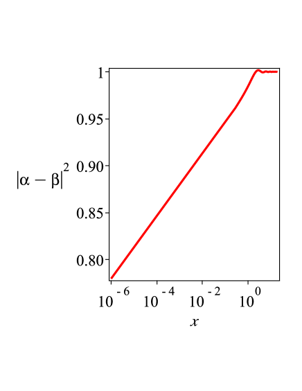
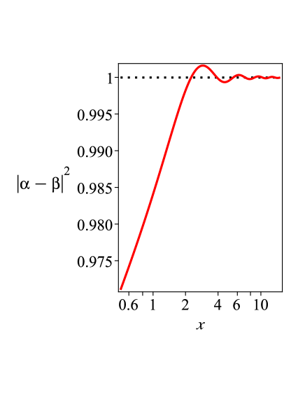
Figure 3: Here we plot the transfer function given by Eq. (47) with $\Lambda_{-}=45$ and $\Lambda_{+}=40$. For large scales, $x\ll 1$, it has a monotonic behavior as indicated by Eq. (49) whereas for small scales, $x\gg 1$, it has an oscillatory behavior approaching the unity. The transition takes place for intermediate scales, $x\simeq 1$, modes which leave the horizon around the time of branes annihilation.

The effects of branes collision and particles creation in the power spectrum Eq. (43) are encoded in the transfer function $\left|\beta-\alpha\right|^{2}$. In the absence of any feature, $\alpha=1,\beta=0$ so we obtain the standard single field DBI inflation Alishahiha:2004eh . Below we would like to investigate the behavior of the transfer function $\left|\beta-\alpha\right|^{2}$ for different modes. Using the explicit formulae of $\alpha$ and $\beta$ given in Eq. (III.2) one obtains

$$\left|\beta-\alpha\right|^{2}=\frac{\pi^{2}}{4}\left[\left(J_{\mu_{+}}J^{\prime}_{\mu_{-}}-J^{\prime}_{\mu_{+}}J_{\mu_{-}}\right)^{2}+\left(J_{\mu_{+}}Y^{\prime}_{\mu_{-}}-J^{\prime}_{\mu_{+}}Y_{\mu_{-}}\right)^{2}\right]x^{2}\,.$$ (47)

As mentioned before we have defined $x\equiv-c_{s}k\tau_{c}=k/k_{c}$ where $k_{c}$ represents the critical mode which leaves the sound horizon at the time of branes collision during inflation. One can check that in the absence of any feature, corresponding to $\mu_{-}=\mu_{+}$, one obtains $\left|\beta-\alpha\right|^{2}=1$ as expected. As mentioned previously, the effects of branes annihilation and particles creations are such that $\Delta\mu\neq 0$ where $\Delta\mu\equiv\mu_{+}-\mu_{-}$.

The spectral index is also modified in the presence of the transfer function as follows

$$n_{\cal R}-1=n_{\cal R}^{0}-1+x\frac{d}{dx}\left|\beta-\alpha\right|^{2}\,.$$ (48)

Now let us look at the shape of the transfer function for different length scales. In Fig. 3 we have plotted the transfer function. As a measure of the length scales of the perturbations, we note that $x=1$ corresponds to the critical mode $k=k_{c}$ which leaves the sound horizon right at the time of branes annihilation. Then depending on whether the mode of interest leaves the sound horizon before the collision or after the collision one respectively has $x\ll 1$ or $x\gg 1$.

First consider the super-horizon scales, $x\ll 1$. This corresponds to modes which leave the sound horizon before the collision. Using the small argument limit of the Bessel functions we obtain

$$\left|\beta-\alpha\right|^{2}\simeq\frac{\Gamma^{2}(\mu_{-})}{4\Gamma^{2}(\mu_{+}+1)}\left(\mu_{-}+\mu_{+}\right)^{2}\left(\frac{x}{2}\right)^{2\Delta\mu}\,.$$ (49)

Our background is such that $\Lambda_{+}<{\Lambda_{-}}$ due to branes collision and energy transfer into radiation so $\Delta\mu>0$. As a result the transfer function scales monotonically for super-horizon modes. Correspondingly, the change in spectral index is obtained to be

$$\Delta n_{\cal R}\equiv n_{\cal R}-n_{\cal R}^{0}\simeq 2\Delta\mu\,.$$ (50)

We see from Eq. (50) that the spectral index for the super-horizon scales become more blue-tilted as compared to the background spectral index. This can also be seen in Fig. 4.

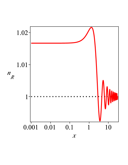
Figure 4: Here we plot the spectral index $n_{\cal R}$. For super-horizon modes, $x\ll 1$, our analytical formula Eq. (48) gives a very accurate prediction for $n_{\cal R}$. For small scales, $x\gg 1$, the oscillatory behavior of $n_{\cal R}$ is clearly seen as suggested by Eq. (47) where $n_{\cal R}$ approaches its background value $n_{\cal R}^{0}$ denoted by the dotted line. The transition takes place around $x\simeq 1$ for modes which leave the horizon around the time of branes annihilation. The parameters are as in Fig. 3

.

Now consider the sub-horizon modes, corresponding to $x\gg 1$. These are the modes which are deep inside the sound horizon at the time of branes collision. Physically one expects these modes to live in their local Minkowski background and should not be affected by branes collision and particles creation. Indeed, using the large argument limit of the Bessel functions $J_{\nu}(z)\simeq\sqrt{\frac{2}{\pi z}}\cos\left(z-(\nu+\frac{1}{2})\frac{\pi}{2}\right)$ and $Y_{\nu}(z)\simeq\sqrt{\frac{2}{\pi z}}\sin\left(z-(\nu+\frac{1}{2})\frac{\pi}{2}\right)$ for $z\gg 1$ we find

$$\left|\beta-\alpha\right|^{2}\simeq 1+{\cal O}(x^{-2})\,.$$ (51)

As expected the transfer function approaches unity so $n_{\cal R}\simeq n_{\cal R}^{0}$. However, both the transfer function and the spectral index are superimposed by oscillatory modulations with decaying amplitude Contaldi:2003zv ; Romano:2008rr ; Zarei:2008nr .

The most interesting effects of branes annihilation and particles creation is on the intermediate scales, $x\simeq 1$. These are the modes which leave the sound horizon around the time of branes collision. In Figures 3 and 4 we have plotted the transfer function and the spectral index. As can be seen, for super-horizon scales the transfer function is monotonically increasing whereas for small scales it oscillates around unity. Correspondingly, the spectral index for super-horizon scales is well approximated by Eq. (50) whereas for small scales it oscillates around $n_{\cal R}^{0}$. The non-trivial transition, happening at the intermediate scales, can be seen in both figures.

As discussed before, the effects of branes annihilation and particles creation result in $\Delta\mu\neq 0$. So far in the perturbations analysis we kept $\mu_{\pm}$ and $\Lambda_{\pm}$ undetermined. Now let us specify $\Delta\mu$ in terms of our background model parameters. Starting with Eqs. (14), (21) and (33) we obtain

$$\Delta\mu=\mu_{+}-\mu_{-} \simeq \frac{3}{\Lambda_{+}}-\frac{3}{{\Lambda_{-}}}$$ (52)

$$\simeq \frac{3}{2\Lambda_{+}}\frac{p_{1}}{p_{2}}\frac{m_{1}^{2}}{m_{2}^{2}}\,.$$

To get the final result we used the approximation that $\Lambda_{+}\simeq{\Lambda_{-}}$. Physically, this is motivated from the assumption that the energy density associated with stack 1 is subdominant compared to the energy density stored in stack 2 so the energy transferred into radiation is much smaller than the background potential energy density. This assumption is necessary for the consistency of our matching condition. We have neglected the interference of perturbations $\delta\phi_{1}$ and $\delta\rho_{r}$ on the perturbations $\delta\phi_{2}$. As a consequence, we have imposed the simple matching condition (37). For this approximation to be valid, we require that $\rho_{r}/V(\phi_{2})\ll 1$ or equivalently $({\Lambda_{+}}-\Lambda_{-})/{\Lambda_{+}}\ll 1$.

We do not have good theoretical control on the masses $m_{1}$ and $m_{2}$ which were originated from the back-reactions of Kahler moduli stabilization and background fluxes on the mobile branes. As a simple ansatz, we may take $m_{1}\simeq m_{2}$. This corresponds to the case that the back-reactions imposed from the background compactification on a single brane is independent of its position inside the throat. This may not be an unreasonable assumption. With this approximation, the consistency of our approximation requires $p_{1}\ll p_{2}$. Also we are working in the probe brane approximations so the mobile stacks of branes should not deform the background AdS geometry significantly. For this to be the case we also need to impose $p_{1}+p_{2}\ll N$. As an example, taking $\Lambda_{+}=40,p_{1}=1$ and $p_{2}=7$ results in $\Delta n_{\cal R}\simeq 0.01$.

One may also compare $\Delta n_{\cal R}$ induced from branes collision to the ${\cal{O}}(\epsilon_{+}^{2})$ contributions to the background spectral index in Eq. (46). We have $\Delta\mu\simeq 3(\Lambda_{-}-\Lambda_{+})/\Lambda_{+}^{2}\simeq 3(\Lambda_{-}-\Lambda_{+})\epsilon_{+}^{2}$. For a reasonable value of $(\Lambda_{-}-\Lambda_{+})=5$ which was used in our numerical examples in Figures 3 and 4 we have $\Delta\mu\sim 15\epsilon_{+}^{2}$ or $\Delta n_{\cal R}\sim 30\epsilon_{+}^{2}$. This indicates that the contributions of the branes collision to the spectral index is much bigger than the sub-leading ${\cal{O}}(\epsilon_{+}^{2})$ contributions to the background $n_{\cal R}^{0}$.

Observationally the result $\Delta n_{\cal R}>0$ is disfavored Komatsu:2010fb noting that the background spectral index is already nearly scale invariant as seen in Eq. (46). To remedy this problem, it may be necessary to embed the simple model of ultra relativistic DBI inflation here to a generic setup of brane inflation where a period of slow-roll brane inflation takes place before DBI inflation starts. This can help to obtain a red spectral index for large scales whereas for smaller scales the spectral index can be blue as we have here.

V Discussions and Conclusions

In this work we have studied the effects of branes annihilation and particles creation in models of DBI inflation where the branes are moving ultra relativistically. In a typical string theory compactification the process of branes and anti-branes annihilation is a generic phenomenon. It is therefore an interesting question how these collisions can affect the dynamics of inflation which may also be detectable in the sky.

The process of branes annihilation is determined by the dynamics of open string tachyon condensation. In a complicated background, such as the warped throat with background fluxes, this is a non-trivial process. The time-scale of tachyon condensation and branes annihilation is given by the inverse of the warped string mass scale, $m_{s}h(r_{0})^{1/4}$. In our effective field theory approach the Hubble expansion rate is considerably smaller than this mass scale so for practical purposes we can take the process of branes annihilation and particles creation to be instantaneous. In our set up the first inflationary stage is a two-field DBI inflation model. After the first stack of branes is annihilated with the background anti-branes a burst of closed strings modes are created. These particles are rapidly diluted by inflation and we eventually end up with a single field DBI inflation system. In order to connect the perturbations in the second inflationary stage to the perturbations generated before the collision we have to use proper matching conditions. Here are the major simplifications imposed in our analysis. It is assumed that the energy in field $\phi_{1}$, which is annihilated during inflation, is sub-dominant compared to energy stored in field $\phi_{2}$ which carries the second stage of inflation. It is assumed that not only the background energy density in $V_{1}(\phi_{1})$ is transferred into radiation $\rho_{r}$ but also the perturbations carried by $\delta\phi_{1}$ are also transferred into perturbations in radiation, $\delta\rho_{r}$. With these simplifications we can follow the perturbations in $\phi_{2}$ before and after the collision using the simple matching conditions (37). Although we did not take into account the perturbations $\delta\phi_{1}$ and $\delta\rho_{r}$ in our analysis but the effects of branes annihilation and particles creation are present at the level of background. In our analysis this translated into $\Delta\mu$ to be non-zero. Interestingly, this is very similar to model studied in Joy:2007na ; Joy:2008qd where the feature is due to a sudden change in slow-roll parameters. In Joy:2007na ; Joy:2008qd the sudden change in slow-roll parameters was motivated from a phase transition Abolhasani:2010kn during hybrid inflation model Linde:1993cn ; Copeland:1994vg ; GarciaBellido:1996qt . It is very interesting that our model, motivated from a completely different setup, shares the same results.

We have calculated the curvature perturbations power spectrum. The effects of branes annihilation are encoded in the transfer function $\left|\beta-\alpha\right|^{2}$. For super-horizon scales, modes which are outside the sound horizon at the time of collision, the transfer function scales monotonically. Consequently, the spectral index is more blue compared to the background spectral index. On the other hand, for small scales, modes which are inside the sound horizon at the time of collision, the transfer function converges to unity with decaying superimposed oscillatory modulations. The non-trivial transitions in transfer function happen for modes which leave the sound horizon around the time of collision. The superimposed oscillatory modulations can have interesting observational consequences on CMB analysis Joy:2008qd ; Flauger:2009ab ; Biswas:2010si . Furthermore, there are strong constraints from non-Gaussianity bounds on standard DBI inflation Shandera:2006ax ; Bean:2007eh ; Bean:2007hc . It would be interesting to calculate the level of non-Gaussianities produced in our setup to put further constraints on the model parameters.

Our results here should be compared with the results obtained in Battefeld:2010rf where similar problem was studied but in the context of slow-roll brane inflation. In Battefeld:2010rf , like here, it was assumed that the perturbations $\delta\phi_{1}$ are transferred into $\delta\rho_{r}$. However, in Battefeld:2010rf the matching conditions (36) have been used instead of the simple matching conditions (37). As a result, the transfer function for large and intermediate scales in Battefeld:2010rf share the same behavior as in our case here. However, in Battefeld:2010rf (see also Flauger:2009ab ; Biswas:2010si ; Flauger:2010ja ), the transfer function for small scales has a constant oscillatory modulation whereas in our case the amplitude of oscillations decays for these modes. For physical reasons, one expects that small scales should be blind to the process of branes annihilation and particles creation so the transfer function is expected to approach unity for these modes. To remedy this problem several methods were put forward in Battefeld:2010rf . Our approach to use the matching conditions (37) may be interpreted as a pragmatic approach towards the methods speculated in Battefeld:2010rf .

To simplify our analysis we considered the model where the branes are moving ultra relativistically. In practice one expects that a successful brane inflation model consists both stages of slow-roll and fast-roll brane inflation. It is possible that during early stage of inflation the branes are moving slowly so one may get a few dozens of e-foldings during the slow-roll regime Kachru:2003sx . As the branes are moving towards the bottom of the throat they reach the speed limit and one should use the DBI inflation methods as we used in this work. The process of branes annihilation and particles creation can happen either during slow-roll regime, as in Battefeld:2010rf , during the ultra relativistic fast-roll limit, as in our case here, or in between these two stages. In the third case, one can not perform analytical studies and a numerical investigation is necessary. It would be interesting to study the effects of branes annihilation in a generic model of brane inflation containing both stages of slow-roll inflation and DBI inflation.

References

References

-
(1)
A. H. Guth,
“The Inflationary Universe: A Possible Solution To The Horizon And Flatness
Problems,”
Phys. Rev. D 23, 347 (1981);
A. D. Linde, “A New Inflationary Universe Scenario: A Possible Solution Of The Horizon, Flatness, Homogeneity, Isotropy And Primordial Monopole Problems,” Phys. Lett. B 108, 389 (1982);
A. Albrecht and P. J. Steinhardt, “Cosmology For Grand Unified Theories With Radiatively Induced Symmetry Breaking,” Phys. Rev. Lett. 48, 1220 (1982). - (2) E. Komatsu et al., “Seven-Year Wilkinson Microwave Anisotropy Probe (WMAP) Observations: Cosmological Interpretation,” arXiv:1001.4538 [astro-ph.CO].
- (3) S. H. Henry Tye, “Brane inflation: String theory viewed from the cosmos,” Lect. Notes Phys. 737, 949 (2008) [arXiv:hep-th/0610221].
- (4) J. M. Cline, “String cosmology,” arXiv:hep-th/0612129.
- (5) C. P. Burgess, “Lectures on Cosmic Inflation and its Potential Stringy Realizations,” PoS P2GC, 008 (2006) [Class. Quant. Grav. 24, S795 (2007)] [arXiv:0708.2865 [hep-th]].
- (6) L. McAllister and E. Silverstein, “String Cosmology: A Review,” Gen. Rel. Grav. 40, 565 (2008) [arXiv:0710.2951 [hep-th]].
- (7) D. Baumann and L. McAllister, “Advances in Inflation in String Theory,” arXiv:0901.0265 [hep-th].
- (8) A. Mazumdar and J. Rocher, “Particle physics models of inflation and curvaton scenarios,” arXiv:1001.0993 [hep-ph].
- (9) G. Dvali and S.-H.H. Tye, ”Brane Inflation”, Phys. Lett. B450 (1999) 72, hep-ph/9812483.
- (10) S. H. S. Alexander, “Inflation from D - anti-D brane annihilation,” Phys. Rev. D 65, 023507 (2002) [arXiv:hep-th/0105032].
- (11) C. P. Burgess, M. Majumdar, D. Nolte, F. Quevedo, G. Rajesh and R. J. Zhang, JHEP 07 (2001) 047, hep-th/0105204.
- (12) G. R. Dvali, Q. Shafi and S. Solganik, “D-brane inflation,” hep-th/0105203.
- (13) I. R. Klebanov and M. J. Strassler, “Supergravity and a confining gauge theory: Duality cascades and chiSB-resolution of naked singularities,” JHEP 0008, 052 (2000), hep-th/0007191.
- (14) S. B. Giddings, S. Kachru and J. Polchinski, “Hierarchies from fluxes in string compactifications,” Phys. Rev. D 66, 106006 (2002), hep-th/0105097.
- (15) K. Dasgupta, G. Rajesh and S. Sethi, “M theory, orientifolds and G-flux,” JHEP 9908, 023 (1999) [arXiv:hep-th/9908088].
- (16) L. Randall and R. Sundrum, “A large mass hierarchy from a small extra dimension,” Phys. Rev. Lett. 83, 3370 (1999) [arXiv:hep-ph/9905221].
- (17) S. Kachru, R. Kallosh, A. Linde, J. Maldacena, L. McAllister and S. P. Trivedi, ” Towards inflation in string theory”, JCAP 0310 (2003) 013, hep-th/0308055.
- (18) H. Firouzjahi and S.-H. H. Tye, “Closer towards inflation in string theory,” Phys. Lett. B 584, 147 (2004), hep-th/0312020.
- (19) C. P. Burgess, J. M. Cline, H. Stoica and F. Quevedo, “Inflation in realistic D-brane models,” JHEP 0409, 033 (2004), hep-th/0403119.
- (20) A. Buchel and R. Roiban, “Inflation in warped geometries,” Phys. Lett. B 590, 284 (2004) [arXiv:hep-th/0311154].
- (21) N. Iizuka and S. P. Trivedi, “An inflationary model in string theory,” Phys. Rev. D 70, 043519 (2004), [arXiv:hep-th/0403203].
- (22) H. Firouzjahi and S.-H. H. Tye, “ Brane inflation and cosmic string tension in superstring theory,” JCAP 0503, 009 (2005), hep-th/0501099.
- (23) D. Baumann, A. Dymarsky, I. R. Klebanov, J. M. Maldacena, L. P. McAllister and A. Murugan, “On D3-brane potentials in compactifications with fluxes and wrapped D-branes,” JHEP 0611, 031 (2006) [arXiv:hep-th/0607050].
- (24) C. P. Burgess, J. M. Cline, K. Dasgupta and H. Firouzjahi, “Uplifting and inflation with D3 branes,” JHEP 0703, 027 (2007) [arXiv:hep-th/0610320].
- (25) D. Baumann, A. Dymarsky, I. R. Klebanov and L. McAllister, “Towards an Explicit Model of D-brane Inflation,” JCAP 0801, 024 (2008) [arXiv:0706.0360 [hep-th]].
- (26) F. Chen and H. Firouzjahi, “Dynamics of D3-D7 Brane Inflation in Throats,” JHEP 0811, 017 (2008) [arXiv:0807.2817 [hep-th]].
- (27) J. M. Cline, L. Hoi and B. Underwood, “Dynamical Fine Tuning in Brane Inflation,” JHEP 0906, 078 (2009) [arXiv:0902.0339 [hep-th]].
- (28) D. Battefeld, T. Battefeld, H. Firouzjahi and N. Khosravi, “Brane Annihilations during Inflation,” JCAP 1007, 009 (2010) [arXiv:1004.1417 [hep-th]].
- (29) D. Battefeld, T. Battefeld and A. C. Davis, “Staggered Multi-Field Inflation,” JCAP 0810, 032 (2008) [arXiv:0806.1953 [hep-th]].
- (30) T. Battefeld, “Exposition to Staggered Multi-Field Inflation,” Nucl. Phys. Proc. Suppl. 192-193, 128 (2009) [arXiv:0809.3242 [astro-ph]].
- (31) N. Barnaby, Z. Huang, L. Kofman and D. Pogosyan, “Cosmological Fluctuations from Infra-Red Cascading During Inflation,” Phys. Rev. D 80, 043501 (2009) [arXiv:0902.0615 [hep-th]].
- (32) N. Barnaby and Z. Huang, “Particle Production During Inflation: Observational Constraints and Signatures,” Phys. Rev. D 80, 126018 (2009) [arXiv:0909.0751 [astro-ph.CO]].
- (33) N. Barnaby, “On Features and Nongaussianity from Inflationary Particle Production,” arXiv:1006.4615 [astro-ph.CO];
- (34) N. Barnaby, “Nongaussianity from Particle Production During Inflation,” Adv. Astron. 2010, 156180 (2010) [arXiv:1010.5507 [astro-ph.CO]].
- (35) D. Green, B. Horn, L. Senatore and E. Silverstein, “Trapped Inflation,” Phys. Rev. D 80, 063533 (2009) [arXiv:0902.1006 [hep-th]].
- (36) P. Brax and E. Cluzel, “Trapped Brane Features in DBI Inflation,” arXiv:1010.4462 [hep-th].
- (37) Y. -F. Cai, J. B. Dent, D. A. Easson, “Warm DBI Inflation,” [arXiv:1011.4074 [hep-th]].
- (38) M. Alishahiha, E. Silverstein and D. Tong, “DBI in the sky,” Phys. Rev. D 70, 123505 (2004) [arXiv:hep-th/0404084].
- (39) C. P. Herzog, I. R. Klebanov and P. Ouyang, “Remarks on the warped deformed conifold,” arXiv:hep-th/0108101.
- (40) X. Chen, “Multi-throat brane inflation,” Phys. Rev. D 71, 063506 (2005) [arXiv:hep-th/0408084].
- (41) S. E. Shandera and S. H. Tye, “Observing brane inflation,” JCAP 0605, 007 (2006) [arXiv:hep-th/0601099].
- (42) R. Bean, X. Chen, H. Peiris and J. Xu, “Comparing Infrared Dirac-Born-Infeld Brane Inflation to Observations,” Phys. Rev. D 77, 023527 (2008) [arXiv:0710.1812 [hep-th]].
- (43) R. Bean, S. E. Shandera, S. H. Henry Tye and J. Xu, “Comparing Brane Inflation to WMAP,” JCAP 0705, 004 (2007) [arXiv:hep-th/0702107].
- (44) X. Chen, M. x. Huang, S. Kachru and G. Shiu, “Observational signatures and non-Gaussianities of general single field inflation,” JCAP 0701, 002 (2007) [arXiv:hep-th/0605045].
- (45) S. Thomas and J. Ward, “IR Inflation from Multiple Branes,” Phys. Rev. D 76, 023509 (2007) [arXiv:hep-th/0702229].
- (46) I. Huston, J. E. Lidsey, S. Thomas and J. Ward, “Gravitational Wave Constraints on Multi-Brane Inflation,” JCAP 0805, 016 (2008) [arXiv:0802.0398 [hep-th]].
- (47) Y. F. Cai and W. Xue, “N-flation from multiple DBI type actions,” Phys. Lett. B 680, 395 (2009) [arXiv:0809.4134 [hep-th]]; Y. F. Cai and H. Y. Xia, “Inflation with multiple sound speeds: a model of multiple DBI type actions and non-Gaussianities,” Phys. Lett. B 677, 226 (2009) [arXiv:0904.0062 [hep-th]]; D. Langlois, S. Renaux-Petel, D. A. Steer and T. Tanaka, “Primordial fluctuations and non-Gaussianities in multi-field DBI inflation,” Phys. Rev. Lett. 101, 061301 (2008) [arXiv:0804.3139 [hep-th]]; D. Langlois, S. Renaux-Petel, D. A. Steer and T. Tanaka, “Primordial perturbations and non-Gaussianities in DBI and general multi-field inflation,” Phys. Rev. D 78, 063523 (2008) [arXiv:0806.0336 [hep-th]]. S. Renaux-Petel, “Combined local and equilateral non-Gaussianities from multifield DBI inflation,” JCAP 0910, 012 (2009) [arXiv:0907.2476 [hep-th]]. M. x. Huang, G. Shiu and B. Underwood, “Multifield DBI Inflation and Non-Gaussianities,” Phys. Rev. D 77, 023511 (2008) [arXiv:0709.3299 [hep-th]]. S. Mizuno, F. Arroja and K. Koyama, “On the full trispectrum in multi-field DBI inflation,” Phys. Rev. D 80, 083517 (2009) [arXiv:0907.2439 [hep-th]]; S. Mizuno, F. Arroja, K. Koyama and T. Tanaka, “Lorentz boost and non-Gaussianity in multi-field DBI-inflation,” Phys. Rev. D 80, 023530 (2009) [arXiv:0905.4557 [hep-th]].
- (48) N. T. Jones, L. Leblond and S. H. H. Tye, “Adding a brane to the brane anti-brane action in BSFT,” JHEP 0310, 002 (2003) [arXiv:hep-th/0307086].
- (49) N. T. Jones and S. H. H. Tye, “An improved brane anti-brane action from boundary superstring field theory and multi-vortex solutions,” JHEP 0301, 012 (2003) [arXiv:hep-th/0211180].
- (50) N. Barnaby, C. P. Burgess, J. M. Cline, “Warped reheating in brane-antibrane inflation,” JCAP 0504, 007 (2005). [hep-th/0412040].
- (51) L. Kofman, P. Yi, “Reheating the universe after string theory inflation,” Phys. Rev. D72, 106001 (2005). [hep-th/0507257].
- (52) H. Firouzjahi, S. -H. H. Tye, “The Shape of gravity in a warped deformed conifold,” JHEP 0601, 136 (2006). [hep-th/0512076].
- (53) X. Chen, S. -H. H. Tye, “Heating in brane inflation and hidden dark matter,” JCAP 0606, 011 (2006). [hep-th/0602136].
- (54) J. Garriga and V. F. Mukhanov, “Perturbations in k-inflation,” Phys. Lett. B 458, 219 (1999) [arXiv:hep-th/9904176].
- (55) N. Deruelle and V. F. Mukhanov, “On matching conditions for cosmological perturbations,” Phys. Rev. D 52, 5549 (1995) [arXiv:gr-qc/9503050].
- (56) J. Martin and D. J. Schwarz, “The influence of cosmological transitions on the evolution of density perturbations,” Phys. Rev. D 57, 3302 (1998) [arXiv:gr-qc/9704049].
- (57) I. Zaballa and M. Sasaki, “Boosted perturbations at the end of inflation,” arXiv:0911.2069 [astro-ph.CO].
- (58) D. H. Lyth, K. A. Malik, M. Sasaki and I. Zaballa, “Forming sub-horizon black holes at the end of inflation,” JCAP 0601, 011 (2006) [arXiv:astro-ph/0510647].
- (59) I. Zaballa, A. M. Green, K. A. Malik and M. Sasaki, “Constraints on the primordial curvature perturbation from primordial black holes,” JCAP 0703, 010 (2007) [arXiv:astro-ph/0612379].
- (60) M. Joy, V. Sahni and A. A. Starobinsky, “A New Universal Local Feature in the Inflationary Perturbation Spectrum,” Phys. Rev. D 77, 023514 (2008) [arXiv:0711.1585 [astro-ph]].
- (61) D. Baumann and L. McAllister, “A Microscopic Limit on Gravitational Waves from D-brane Inflation,” Phys. Rev. D 75, 123508 (2007) [arXiv:hep-th/0610285].
- (62) C. R. Contaldi, M. Peloso, L. Kofman et al., “Suppressing the lower multipoles in the CMB anisotropies,” JCAP 0307, 002 (2003). [astro-ph/0303636].
- (63) A. E. Romano and M. Sasaki, “Effects of particle production during inflation,” Phys. Rev. D 78, 103522 (2008) [arXiv:0809.5142 [gr-qc]].
- (64) M. Zarei, “Short Distance Physics and Initial State Effects on the CMB Power Spectrum and Cosmological Constant,” Phys. Rev. D 78, 123502 (2008) [arXiv:0809.4312 [hep-th]].
- (65) M. Joy, A. Shafieloo, V. Sahni and A. A. Starobinsky, “Is a step in the primordial spectral index favored by CMB data ?,” JCAP 0906, 028 (2009) [arXiv:0807.3334 [astro-ph]].
- (66) A. A. Abolhasani, H. Firouzjahi and M. H. Namjoo, “Curvature Perturbations and non-Gaussianities from Waterfall Phase Transition during Inflation,” arXiv:1010.6292 [astro-ph.CO].
- (67) A. D. Linde, “Hybrid inflation,” Phys. Rev. D 49, 748 (1994) [arXiv:astro-ph/9307002].
- (68) E. J. Copeland, A. R. Liddle, D. H. Lyth, E. D. Stewart and D. Wands, “False vacuum inflation with Einstein gravity,” Phys. Rev. D 49, 6410 (1994) [arXiv:astro-ph/9401011].
- (69) J. Garcia-Bellido, A. D. Linde and D. Wands, “Density perturbations and black hole formation in hybrid inflation,” Phys. Rev. D 54, 6040 (1996) [arXiv:astro-ph/9605094].
- (70) R. Flauger, L. McAllister, E. Pajer, A. Westphal and G. Xu, “Oscillations in the CMB from Axion Monodromy Inflation,” arXiv:0907.2916 [hep-th].
- (71) T. Biswas, A. Mazumdar and A. Shafieloo, “Wiggles in the cosmic microwave background radiation: echoes from non-singular cyclic-inflation,” arXiv:1003.3206 [hep-th].
- (72) R. Flauger and E. Pajer, “Resonant Non-Gaussianity,” arXiv:1002.0833 [hep-th].