The Shape and Profile of the Milky Way Halo as Seen by the Canada-France-Hawaii Telescope Legacy Survey

Abstract

We use Canada$-$France$-$Hawaii Telescope Legacy Survey data for 170 deg², recalibrated and transformed to the Sloan Digital Sky Survey $ugri$ photometric system, to study the distribution of near-turnoff main-sequence stars in the Galactic halo along four lines of sight to heliocentric distances of $\sim 35$ kpc. We find that the halo stellar number density profile becomes steeper at Galactocentric distances greater than $R_{\rm gal}\sim 28$ kpc, with the power law index changing from $n_{\rm inner}=-2.62\pm 0.04$ to $n_{\rm outer}=-3.8\pm 0.1$. In particular, we test a series of single power law models and find them to be strongly disfavored by the data. The parameters for the best-fit Einasto profile are $n=2.2\pm 0.2$ and $R_{\rm e}=22.2\pm 0.4$ kpc. We measure the oblateness of the halo to be $q\equiv c/a=0.70\pm 0.01$ and detect no evidence of it changing across the range of probed distances. The Sagittarius stream is detected in the $l=173\arcdeg$ and $b=-62\arcdeg$ direction as an overdensity of ${\rm[Fe/H]}\sim-1.5$ dex stars at $R_{\rm gal}\sim 32$ kpc, providing a new constraint for the Sagittarius stream and dark matter halo models. We also detect the Monoceros stream as an overdensity of ${\rm[Fe/H]}>-1.5$ dex stars in the $l=232\arcdeg$ and $b=26\arcdeg$ direction at $R_{\rm gal}\lesssim 25$ kpc. In the two sightlines where we do not detect significant substructure, the median metallicity is found to be independent of distance within systematic uncertainties (${\rm[Fe/H]}\sim-1.5\pm 0.1$ dex).

1 Introduction

Studies of the Galactic stellar halo set constraints on the formation history of the Milky Way and galaxy formation processes in general. For example, contemporary simulations of galaxy formation predict that stellar halos of Milky-Way-type galaxies are assembled from inside out, with the majority of mass ($50\%-80\%$) coming from several massive ($10^{8}$$-$$10^{10}$ $M_{\sun}$) satellites that have merged more than 9 Gyr ago, while the remaining mass comes from lower mass satellites accreted in the past 5$-$9 Gyr (Bullock & Johnston, 2005; De Lucia & Helmi, 2008). The actual fraction of massive versus less massive mergers will depend on the formation history of the galaxy in question.

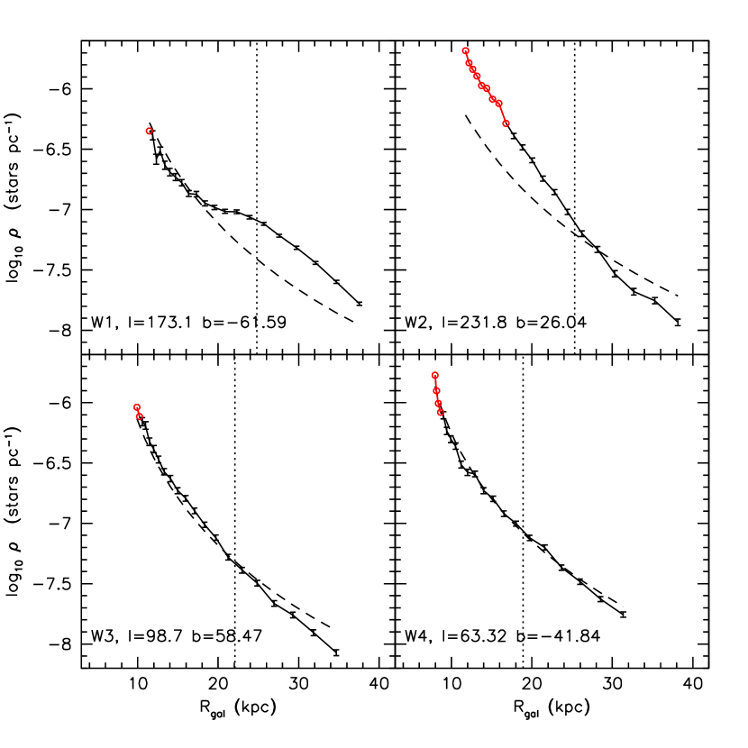
Figure 9: Stellar number density, measured in four CFHTLS wide-area survey beams as a function of distance from the Galactic center, $R_{gal}$. Open circles denote the measurements within 5 kpc of the Galactic plane, where the contamination by disk stars may be greater than 10%. For clarity, the symbols have been connected by solid lines. Overplotted as a dashed line is the oblate power law halo model from J08. Its overall normalization has been adjusted to fit the W3 and W4 data at $R_{gal}<25$ kpc, as well as W1 data points satisfying $R_{gal}<15$ kpc (to avoid contamination by the Sagittarius stream). The vertical line shows the J08 distance limit. The excess density at $R_{\rm gal}\gtrsim 15$ kpc in the W1 field can be associated with the Sagittarius stream, while the overdensity at $R_{\rm gal}\lesssim 25$ kpc in the W2 beam is consistent with the location of the Monoceros stream.

A further prediction is that the stellar halos should be more centrally concentrated and should have steeper density profiles at moderate radii ($>20-30$ kpc), than host dark matter halos (e.g., Figure 9 in Bullock & Johnston 2005 or Figure 12 in De Lucia & Helmi 2008). According to Bullock & Johnston (2005), “the difference in profile shapes—and the steep rollover in the light matter at moderate to large radii—is a natural consequence of embedding the light matter deep within the dark matter satellites: the satellites’ orbits can decay significantly before any of the more tightly bound material is lost.” Hence, they anticipate a correlation between the extent of the stellar halo (steepness of the density profile) and the extent (or mass) of satellites that built the halo: less extended (more massive) satellites will build more concentrated stellar halos. Therefore, the contribution of massive mergers to the formation of the Milky Way halo can be constrained by characterizing the stellar halo number density profile over large distances and over a wide sky area.

The large area covered by the Sloan Digital Sky Survey (SDSS; York et al. 2000), with accurate photometric measurements ($\sim 0.02$ mag, Ivezić et al. 2004) and faint flux limits ($r<22$), allowed for a novel approach to studies of the stellar distribution in the Galaxy. Using a photometric parallax relation appropriate for main-sequence stars, Jurić et al. (2008, hereafter J08) estimated distances for a large number of stars and directly mapped the Galactic stellar number density to heliocentric distances of 20 kpc. They found that the halo stellar number density distribution within 20 kpc of the Sun can be fit with a two parameter, single power-law ellipsoid model

$$\rho(R,Z)\propto[R^{2}+(Z/q)^{2}]^{n/2},$$ (1)

where $R$ and $Z$ are the cylindrical galactocentric radius and height above the Galactic plane, respectively, $n=-2.77\pm 0.2$ is the power law index, and $q\equiv c/a=0.64\pm 0.1$ is the ratio of major axes in the $Z$ and $R$ direction, indicating that the halo is oblate (flattened in the $Z$ direction). However, additional data suggest that the J08 single power law halo cannot be extrapolated beyond 20 kpc. A kinematic analysis by Carollo et al. (2007, 2010) suggests that the halo consists of two components with different spatial density profiles and median metallicities, with the “inner” to “outer” halo transition happening at 15-20 kpc, and the density profile becoming shallower beyond that point. On the other hand, the distribution of RR Lyrae stars from the SEKBO survey (Keller et al., 2008), and RR Lyrae and main-sequence stars from SDSS stripe 82 data seem to show a steeper density profile beyond 30 kpc (main sequence stars can be detected up to 40 kpc in coadded SDSS stripe 82; Sesar et al. 2010).

While these studies indicate a change in the halo density profile, each has its shortcomings: kinematic studies do not give a direct measurement of the density profile but rather model it under an assumed dark matter halo potential, RR Lyrae stars are relatively sparse tracers of stellar number density ($\sim 5$ kpc^-3 in the solar neighborhood; Sesar et al. 2010 and references therein), and the SDSS stripe 82 region covers only about $1\%$ of the sky. Ideally, the halo stellar number density distribution should be mapped using main-sequence stars over a large fraction of the sky and to a distance of at least 50 kpc. Such studies will be enabled by next generation wide-area surveys such as the Dark Energy Survey (Lin et al., 2009), Pan-STARRS (Kaiser et al., 2002) and Large Synoptic Survey Telescope (LSST; Ivezić et al. 2008b; LSST Science Book 2009).

Meanwhile, the Canada-France-Hawaii Telescope Legacy Survey (CFHTLS) has observed 170 deg² of sky in four fields as part of CFHTLS “wide” survey. The names, positions, and sky coverage of CFHTLS “Wide” fields are listed in Table 1. Due to their relatively small sky coverage, these fields are effectively “pencil-beam” surveys for the purposes of this paper. Despite the small sky coverage (comparable to SDSS stripe 82), these data are very useful because of their depth (95% completeness at $i^{\prime}=23.5$ for point sources; Goranova et al. 2009), corresponding to a distance limit of $\sim 35$ kpc for main-sequence stars, and because they observe lines of sight unexplored by other surveys. These properties allow one to study how the halo density profile changes as a function of distance and line of sight, both in the inner and outer halo.

This paper is organized as follows. In Section 2, we give an overview of CFHTLS data and describe the synthesis of SDSS $ugri$ magnitudes from recalibrated CFHTLS $u^{*}g^{\prime}r^{\prime}i^{\prime}i^{\prime}_{2}$ observations. The recalibration and transformation of CFHTLS data into the SDSS photometric system (Fukugita et al., 1996) is done to allow the usage of CFHTLS data with relations already defined on the SDSS system, such as the color-luminosity and photometric metallicity relations (Ivezić et al., 2008a; Bond et al., 2010). The CFHTLS $z^{\prime}$-band observations are not recalibrated as they were not publicly available for all CFHTLS fields at the time of writing. In Section 3, we analyze the distribution of stellar counts as a function of position and compare it to the J08 halo model. The best-fit broken power-law model is derived in Section 4. In Section 5, we study the metallicity distribution in the halo and analyze the dependence of best-fit model parameters on the adopted metallicity distribution. We finish by discussing our conclusions in Section 6.

2 The Data

We perform several data quality tests and post-processing steps before using the CFHTLS data in scientific analysis. First, we photometrically recalibrate the data by utilizing repeated CFHTLS observations and then transform them to the SDSS photometric system. We also investigate the performance of different types of CFHTLS magnitudes.

2.1 Overview of CFHTLS Data

We use the CFHTLS data processed by the MegaPipe image processing pipeline (Gwyn, 2008). The pipeline takes as input MegaCam (Boulade et al., 2003) images detrended by the Elixir pipeline (Magnier & Cuillandre, 2004), and performs an astrometric and photometric calibration on them. The calibrated images are resampled and combined into image stacks. The catalogs of sources are derived by running SExtractor (Bertin & Arnouts, 1996) on each image stack. The resulting catalogs only pertain to a single band; no multi-band catalogs are generated by the MegaPipe pipeline. The astrometry in these catalogs is accurate to within $0\arcsec.2$ relative to external reference frames (Gwyn, 2008). The catalogs are available for each pointing (a $\sim 1$ deg² part of a CFHTLS field) through the Canadian Astronomy Data Centre (CADC) Web site.

Since multi-band catalogs are not available, we generate them for each pointing by positionally matching sources detected in $u^{*}g^{\prime}r^{\prime}$ bands to sources detected in the $i^{\prime}$ or $i^{\prime}_{2}$ band using a $1\arcsec.5$ matching radius. The $i^{\prime}$ and $i^{\prime}_{2}$ bands are the deepest of the CFHT bands, so most objects detected in other bands will also be detected in these two. The $i^{\prime}_{2}$ filter is the new CFHT filter that was installed after the $i^{\prime}$ filter broke in 2007 October. We further match $\sim 1.7$ million CFHTLS sources overlapping the SDSS footprint to SDSS DR7 data (Abazajian et al., 2009) using the $1\arcsec.5$ matching radius.

2.2 Star-Galaxy Separation

We separate point-like and extended sources using the half-light-radius (HLR) measured (in pixel units) for each detected source by the SExtractor. For point-like sources, the HLR is independent of magnitude and depends only on image seeing (Schultheis et al., 2006). For each CFHTLS band and pointing, we remove the dependence of HLR on image seeing by subtracting the median HLR value of bright (17.5$-$18.5 mag) sources. Bright sources are used in this procedure because they are dominated by point-like sources (see Figure 9 in Gwyn 2008). We find that after subtraction, the distribution of HLR values of bright sources in the $r^{\prime}$ and $i^{\prime}$ (or $i^{\prime}_{2}$) bands can be modeled as a $\sim 0.1$ pixel wide Gaussian centered at zero.

We classify a source as a star if its HLR in the $r^{\prime}$ and $i^{\prime}$ (or $i^{\prime}_{2}$) bands is less than 0.2 pixels (after removing the dependence of HLR on image seeing). Sources that do not satisfy this condition are classified as galaxies. To estimate the quality of this classification, we compare it to the SDSS star-galaxy classification (Lupton et al., 2002) based on deep, co-added SDSS stripe 82 data. The star-galaxy separation in co-added SDSS stripe 82 data is reliable to at least $r\sim 23$ (Annis, J. et al.(2011), in preparation), and for purposes of this comparison we consider it to be the ground truth.

Figure 1 shows the fraction of SDSS stars identified as stars in CFHTLS data (completeness) and the fraction of CFHTLS stars identified as galaxies by the SDSS (contamination) as a function of $r^{\prime}$ magnitude. Using this plot, we estimate that the observed number counts will be underestimated by about $5\%$ for $r^{\prime}<21$ and overestimated by about 15%$-$20% at the faint end ($r^{\prime}\sim 22.5$).

2.3 Recalibration and Transformation of CFHTLS Data to the SDSS $ugriz$ Photometric System

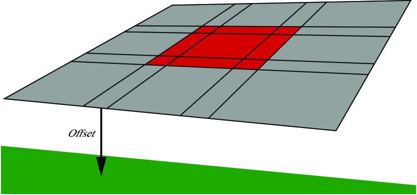
Figure 2: Schematic of the calibration process. For relative calibration (top), the pointings within a CFHTLS field (9 tiles) are recalibrated to a photometric system specific to that field using $\Delta_{j}^{rel}$ offsets (see Section 2.3.2 for details). For absolute calibration (bottom), the field is calibrated to the SDSS system (light/green plane) using a $\Delta_{f}^{abs}$ offset (see Section 2.3.3 for details).

Following Padmanabhan et al. (2008), the photometric recalibration of CFHTLS data is separated into “relative” and “absolute” calibration. This process is schematically illustrated in Figure 2. For relative calibration, we use overlaps between pointings to recalibrate all pointings within a CFHTLS field onto a single photometric system (specific to that field). This calibration is then tied to the SDSS photometric system (absolute calibration). The final step in the process is the synthesis of SDSS $ugri$ photometry from recalibrated CFHTLS $u^{*}g^{\prime}r^{\prime}i^{\prime}i^{\prime}_{2}$ observations.

2.3.1 Flux Extraction

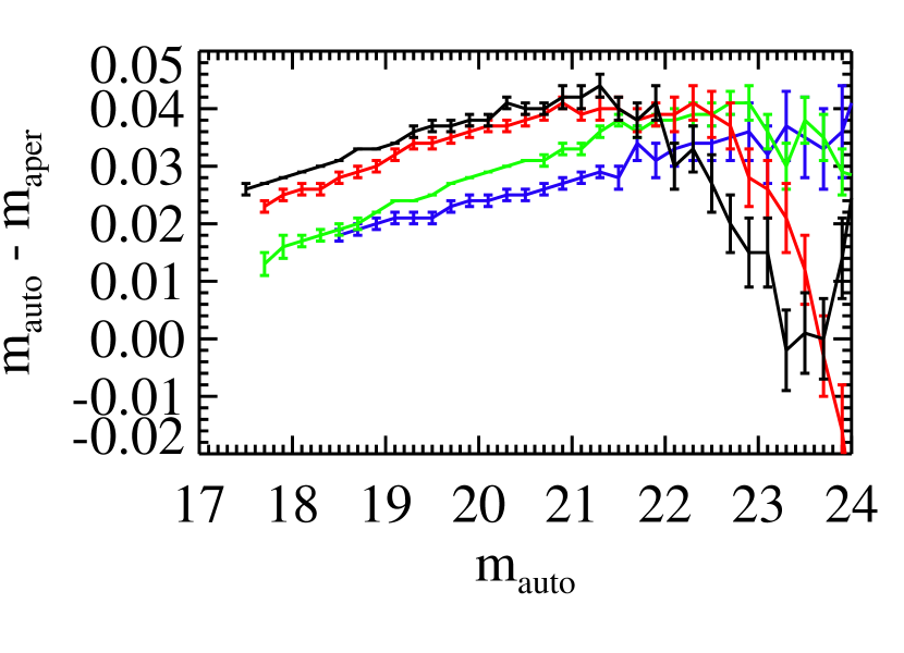
Figure 3: Dependence of $m_{auto}-m_{aper}$ residuals of stars on $m_{auto}$, where $m_{auto}$ are adaptive-aperture magnitudes, $m_{aper}$ are fixed-aperture magnitudes, and $m$ stands for $u^{*}$, $g^{\prime}$, $r^{\prime}$, and $i^{\prime}$ bands (blue, green, red, and black lines, respectively).

The CFHTLS catalogs provide adaptive-aperture ($m_{auto}$) and fixed-aperture magnitudes ($m_{aper}$) for sources detected by SExtractor. To compare fluxes extracted by these two methods, we select stars from the W3 field and calculate $m_{auto}-m_{aper}$ residuals, where $m$ stands for $u^{*}$, $g^{\prime}$, $r^{\prime}$, and $i^{\prime}$ bands. The residuals are binned in $m_{auto}$ bins and median values are calculated for each bin. The dependence of median values on $m_{auto}$ for $u^{*}g^{\prime}r^{\prime}i^{\prime}$ bands is shown in Figure 3. In general, we find that the median difference between adaptive- and fixed-aperture magnitudes increases linearly towards fainter magnitudes, reaching $\sim 0.04$ mag in the $i^{\prime}$ band.

This indicates that there is a problem with one or both extraction methods. As we will demonstrate in Section 2.4, the adaptive-aperture magnitudes ($m_{auto}$) are responsible for the dependence seen in Figure 3, based on the following reasons. First, measuring adaptive-aperture magnitudes is a more complex process than measuring at the fixed aperture (for details see SExtractor v2.5 manual), making adaptive-aperture magnitudes less robust. Second, a caveat in the SExtractor v2.5 manual warns of potential problems with adaptive-aperture magnitudes when the SExtractor $R_{min}$ parameter is set too low. This caveat states that, “when signal to noise is low, it may appear that an erroneously small aperture is taken by the algorithm. That is why we have to bound the smallest accessible aperture to $R_{min}$”. Therefore, if $R_{min}$ was set too low during flux extraction, inadequate (too small) apertures may have been used, making $m_{auto}$ fainter and causing $m_{auto}-m_{aper}$ residuals to be biased towards positive values. Even though the caveat states that this may happen at fainter magnitudes (low signal-to-noise), Figure 3 seems to indicate that brighter magnitudes may be affected as well. We therefore use fixed-aperture magnitudes in the rest of this work.

2.3.2 Relative Calibration

Relative calibration places all pointings within a CFHTLS field onto a single photometric system (specific to that field) using repeatedly observed stars that are located in regions where pointings overlap (CFHTLS pointings overlap about $3\arcsec$ in right ascension and $4\arcsec$ in declination directions). Mathematically, the problem of relative calibration can be described as a $\chi^{2}$ minimization problem (Padmanabhan et al., 2008) with

$$\chi^{2}=\sum^{n_{star}}_{i}\chi^{2}_{i}=\sum^{n_{star}}_{i}\sum_{j\in\mathcal{O}(i)}\left[\frac{m_{i}-m_{j,orig}-\Delta^{rel}_{j,f}}{\sigma_{j}}\right]^{2},$$ (2)

where $n_{star}$ is the number of unique, repeatedly observed stars in the $f=$ W1, W2, W3, W4 field, $j$ runs over multiple observations (pointings), $\mathcal{O}(i)$, of the $i$th star with unknown true magnitude $m_{i}$, $m_{orig}$ and $\sigma$ are the magnitude and its error supplied by MegaPipe, respectively, and $\Delta^{rel}_{j,f}$ is the correction needed to place the $j$th pointing on the $f$ field’s relative photometric system. The system defined with Equation 2 is overdetermined, since the number of unknowns ($n_{star}+n$[parameters]) is smaller than the number of observations ($n_{obs}$ is at least $2n_{star}$). Equation 2 can be expressed in matrix form and can be solved using sparse matrix techniques (see Section 3.2 in Padmanabhan et al. 2008).

To solve Equation 2 for each field, we use repeatedly observed stars with $17<m_{orig}<23$, where $m_{orig}=u^{*},g^{\prime},r^{\prime},i^{\prime},i^{\prime}_{2}$. The observations in this magnitude range are not saturated and their reported photometric errors are smaller than 0.2 mag. The observations are supplied to a sparse matrix inversion code written by Padmanabhan et al. (2008), and the best-fit $\Delta^{rel}_{j,f}$ values returned by this code are renormalized so that the median value of $\Delta^{rel}_{j,f}$ is equal to zero. On average, we find the rms scatter of $\Delta^{rel}_{j,f}$ values to be between 0.02 and 0.03 mag, reflecting the systematic uncertainty in CFHTLS magnitudes.

2.3.3 Absolute Calibration

Following relative calibration, we tie relative photometric systems to the SDSS photometric system using CFHTLS stars matched to SDSS stars. The goal is to find the best-fit $\Delta^{abs}_{f}$ value for each field, such that

$$\chi^{2}=\sum_{f=W1}^{W4}\sum_{i}\left[\frac{m_{i,rel}-m_{i,sdss}-C\,color-\Delta^{abs}_{f}}{\sqrt{\sigma_{i}^{2}+\sigma_{i,sdss}^{2}}}\right]^{2}$$ (3)

is minimized, where $i$ runs over CFHTLS stars in the $f$ field matched to SDSS stars, $m_{rel}$ is the CFHTLS magnitude after relative calibration ($m_{rel}=m_{orig}+\Delta^{rel}_{j,f}$), and $m_{sdss}$ and $\sigma_{sdss}$ are SDSS point-spread function (PSF) magnitude and its error, respectively. For $m_{rel}=u^{*},g^{\prime},r^{\prime},i^{\prime},i^{\prime}_{2}$, the SDSS color and band are color$=u-g,g-r,g-r,r-i,r-i$ and $m_{sdss}=u,g,r,i,i$, respectively (colors and magnitudes are not corrected for interstellar medium (ISM) extinction).

The $C$ color term corrects the linear dependence of $m_{i,rel}-m_{i,sdss}$ residuals on color caused by differences between CFHTLS and SDSS spectral response curves (see Figure 1 in Gwyn 2008 for a comparison of spectral response curves). This term reduces the scatter in $m_{i,rel}-m_{i,sdss}$ residuals and improves our estimate of $\Delta^{abs}_{f}$. Since CFHTLS and SDSS spectral response curves should not change significantly with time, the $C$ color term is simultaneously fit for all four CFHTLS fields. Note that this term is only used when estimating $\Delta^{abs}_{f}$; linear and other higher-order color terms that model the transformation of CFHTLS bands into SDSS bands are derived in Section 2.3.4.

To determine $\Delta^{abs}_{f}$ values, we use CFHTLS stars with $m_{rel}>17$ matched to SDSS stars with $m_{sdss}<21$ and with the SDSS color as specified in Table 2. The best-fit $C$ and $\Delta^{abs}_{f}$ are also listed in Table 2. Finally, we define recalibrated CFHTLS magnitudes as

$$m_{cfht}=m_{j,f,orig}+\Delta^{rel}_{j,f}+\Delta^{abs}_{f}=m_{j,f,orig}+\Delta^{tot}_{j,f},$$ (4)

where $\Delta^{tot}_{j,f}$ is the total correction for the $j$th pointing in the $f$ field. The $\Delta^{tot}_{j,f}$ values for CFHTLS fields are listed in Tables 3.

2.3.4 Transformation to SDSS Bandpasses

With CFHTLS $m_{cfht}=u^{*},g^{\prime},r^{\prime},i^{\prime},i^{\prime}_{2}$ observations calibrated onto the SDSS system, we now derive the equations that transform CFHTLS observations into SDSS $m_{sdss}=u,g,r,i,i$ magnitudes. In general, the transformation from CFHTLS to SDSS bandpasses can be defined as

$$m=m_{cfht}+f(color)+Z_{0},$$ (5)

where $Z_{0}$ is the constant term, and $f(color)$ is some function of CFHT colors (colors and magnitudes are not corrected for ISM extinction).

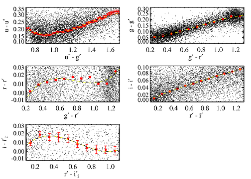
Figure 4: Dependence of $m_{sdss}-m_{cfht}$ residuals on CFHT color, where $m_{sdss}=u,g,r,i,i$ are SDSS PSF magnitudes and $m_{cfht}=u^{*},g^{\prime},r^{\prime},i^{\prime},i^{\prime}_{2}$ are recalibrated CFHTLS magnitudes. The $m_{sdss}-m_{cfht}$ residuals are shown as dots (not all are shown for clarity) and the symbols show their median values in color bins. The error bars show errors in medians. The dashed lines were obtained by fitting polynomials to $m_{sdss}-m_{cfht}$ medians.

To find $f(color)$ and $Z_{0}$ for each SDSS $ugri$ bandpass, we bin $m_{sdss}-m_{cfht}$ residuals as a function of CFHT color, and fit polynomials to $m_{sdss}-m_{cfht}$ medians. Here we only use CFHTLS stars with $m_{cfht}>17$ matched to SDSS stars with $m_{sdss}<20$. The dependence of $m_{sdss}-m_{cfht}$ residuals on CFHT color is shown in Figure 4.

The best-fit polynomials shown in Figure 4 define the transformation of recalibrated CFHTLS magnitudes into SDSS magnitudes:

$$u = u^{*}+1.07-2.375(u^{*}-g^{\prime})+1.954(u^{*}-g^{\prime})^{2}-0.483(u^{*}-g^{\prime})^{3}$$ (6)

$$g = g^{\prime}+0.05-0.062(g^{\prime}-r^{\prime})+0.365(g^{\prime}-r^{\prime})^{2}$$ (7)

$$r = r^{\prime}-0.05+0.275(g^{\prime}-r^{\prime})-0.380(g^{\prime}-r^{\prime})^{2}$$ (8)

$$i = i^{\prime}-0.002+0.092(r^{\prime}-i^{\prime})-0.015(r^{\prime}-i^{\prime})^{2}$$ (9)

$$i = i^{\prime}_{2}-0.005+0.145(r^{\prime}-i^{\prime}_{2})-0.280(r^{\prime}-i^{\prime}_{2})^{2}+0.140(r^{\prime}-i^{\prime}_{2})^{3}.$$ (10)

Using Equations 6 to 10, we synthesize SDSS photometry ($m=u,g,r,i$) for all CFHTLS observations. Note that these transformations can be used even if the relative recalibration step from Section 2.3.2 is skipped because the best-fit $\Delta^{rel}_{j,f}$ values are renormalized so that their median is zero.

2.4 Quality of Photometric Calibration

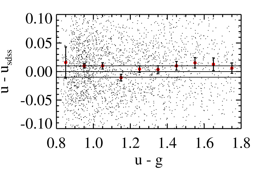
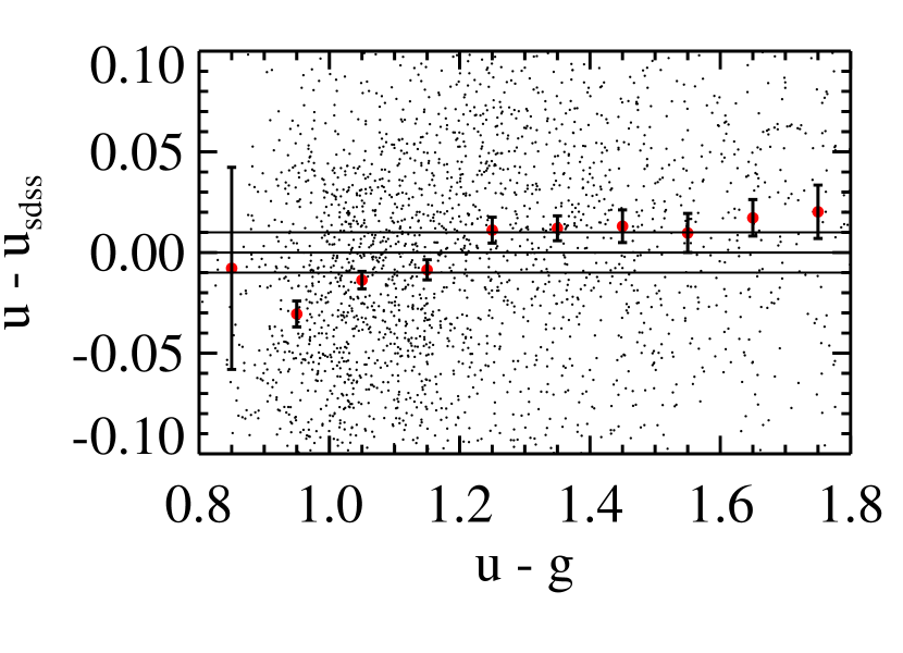
Figure 5: Dependence of $u-u_{sdss}$ residuals (dots) on synthetic $u-g$ color (not corrected for ISM extinction) for the W1 (top) and W2 (bottom) fields, where $u$ and $g$ are synthetic observations derived from recalibrated CFHTLS observations, and $u_{sdss}$ is the SDSS PSF $u$ band magnitude. The symbols show $u-u_{sdss}$ medians in $u-g$ color bins, and error bars show the error in median. To guide the eye, the solid lines show $u-u_{sdss}=\pm 0.01$ mag. For the W1 field, the $u-u_{sdss}$ medians are within 0.02 mag and do not depend on $u-g$ color, while for the W2 field the $u-u_{sdss}$ medians seem to show linear dependence on $u-g$ color for $u-g<1.3$, indicating a possible problem with CFHTLS $u^{*}$ band observations in the W2 field.

To estimate the quality of synthesized photometry, we use CFHT sources brighter than $m=17$ that are matched to SDSS stars with $m_{sdss}<20$, where $m$ stands for $u$, $g$, $r$, and $i$. For each band $m$ we calculate $m-m_{sdss}$ residuals, and bin them as a function of color (not corrected for ISM extinction, color$=u-g,g-r,g-r,r-i$ for $m=u,g,r,i$, respectively). The absolute value of $m-m_{sdss}$ medians for $m=g,r,i$ bands is smaller than 0.01 mag and shows no dependence on color, for all CFHTLS fields. For W1, W3, and W4 fields, the absolute value of $u-u_{sdss}$ medians is smaller than 0.02 mag, and shows no dependence on $u-g$ color, while for the W2 field the $u-u_{sdss}$ medians seem to show linear dependence on $u-g$ color for $u-g<1.3$, as illustrated in Figure 5 (bottom panel). Since all four fields were calibrated using the same procedure, and the transformations from recalibrated CFHTLS to SDSS magnitudes were derived using the data from all fields, the $u-u_{sdss}$ dependence on $u-g$ color points to a problem with the original CFHTLS $u^{*}$-band observations in the W2 field. We hypothesize that the $u-u_{sdss}$ dependence on color may be due to incorrectly determined color-dependent air-mass term by Elixir or MegaPipe pipelines.

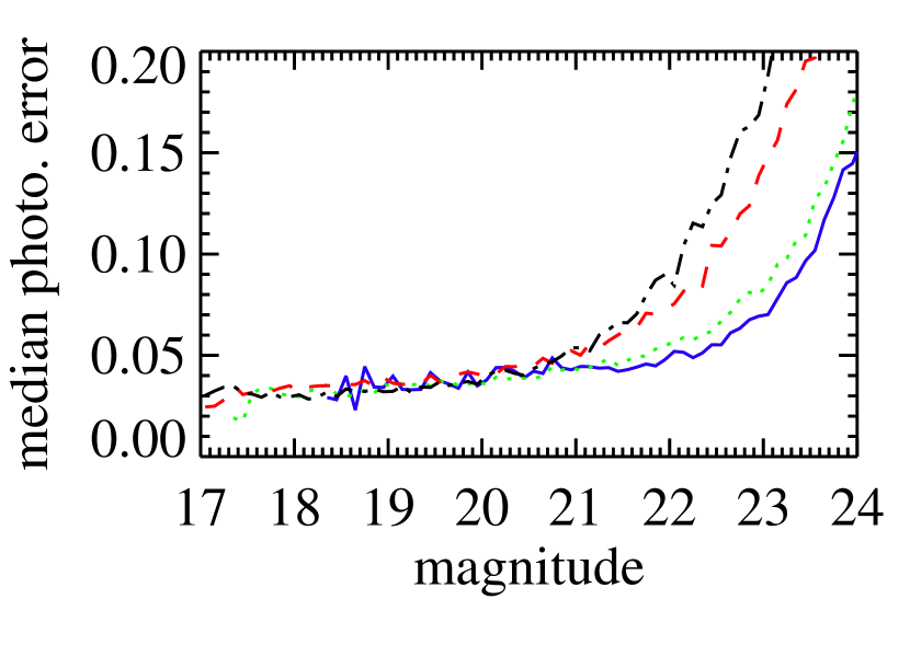
Figure 6: Median photometric error as a function of magnitude for synthetic $u$-band (solid), $g$-band (dotted), $r$-band (dashed), and $i$-band observations (dot-dashed). The median photometric error was calculated as the rms scatter of $m_{2}-m_{1}$ residuals in magnitude bins, where $m_{1}$ and $m_{2}$ are repeated observations of a star. The systematic uncertainty in synthetic $ugri$ magnitudes is $\sim 0.03$ mag, as indicated by the median photometric error at the bright end (magnitudes brighter than $\sim 20$ mag).

The systematic uncertainty of synthesized magnitudes can be determined by comparing synthesized photometry of repeatedly observed CFHT sources; such sources can be found in regions where pointings overlap. We find that the systematic uncertainty is $\sim 0.03$ mag (see Figure 6), which is consistent with the value cited by Gwyn (2008).

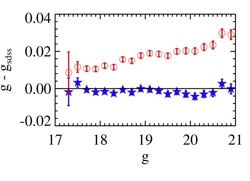
Figure 7: Dependence of median $g-g_{sdss}$ residuals on $g$ magnitude, where $g$ are recalibrated fixed- (stars) and adaptive-aperture CFHTLS magnitudes (open circles), and $g_{sdss}$ is the PSF magnitude measured by SDSS. The error bars indicate errors in medians. This comparison of CFHTLS and SDSS magnitudes shows that the behavior seen in Figure 3 is due to incorrectly measured adaptive-aperture magnitudes. Similar results are obtained for $u$, $r$, and $i$ magnitudes.

To quantify the non-linearity of synthesized photometry, we bin $m-m_{sdss}$ residuals in $m=u,g,r,i$ magnitude bins. As shown in Figure 7, the medians of $g-g_{sdss}$ residuals in $g$ magnitude bins show no dependence on magnitude, indicating linear behavior of synthesized photometry. We have repeated this last test using adaptive-aperture magnitudes and have found a magnitude dependence in $g-g_{sdss}$ residuals similar to the one shown in Figure 3. Similar results are also obtained for $uri$ bands. These results point to the dependence shown in Figure 3 as being due to the problematic adaptive-aperture flux extraction, and justify our choice of fixed-aperture magnitudes.

3 Analysis of the Number Density Distribution Profiles

The data presented in previous sections allow us to measure the stellar number density of near main sequence turnoff (MSTO) halo stars, and examine it as a function of position in the Galaxy. The sample we obtained from the CFHTLS extends to distances and Galactocentric radii ($R_{gal}$) nearly a factor of two greater than previous wide-area studies that used main-sequence stars (e.g., $5\lesssim R_{gal}\lesssim 15$ kpc; J08). The sample also overlaps in range with studies based on RR Lyrae stars ($5\lesssim R_{gal}\lesssim 110$ kpc; Sesar et al. 2010), and it therefore presents an opportunity to examine the behavior of the halo density profile in the intermediate range ($5\lesssim R_{gal}\lesssim 30$ kpc).

We begin by selecting a sample of near-MSTO stars with the following criteria:

$$0.2<g-r<0.3$$ (11)

$$g>17\,\,\&\,\,17<r<22.5\,\,\&\,\,i>17$$ (12)

$$5<D/{\rm kpc}<35$$ (13)

where magnitudes and colors are corrected for ISM extinction using maps from Schlegel, Finkbeiner & Davis (1998). The $g-r$ color cut serves to select near-MSTO stars, and $D$ is the heliocentric distance to a star computed using the photometric-parallax relation from Ivezić et al. (2008a, see Equations A2 and A7 in their Appendix A):

$$M_{r}=-0.56+14.32x-12.97x^{2}+6.127x^{3}-1.267x^{4}+0.0967x^{5}-1.11[Fe/H]-0.18[Fe/H]^{2}.$$ (14)

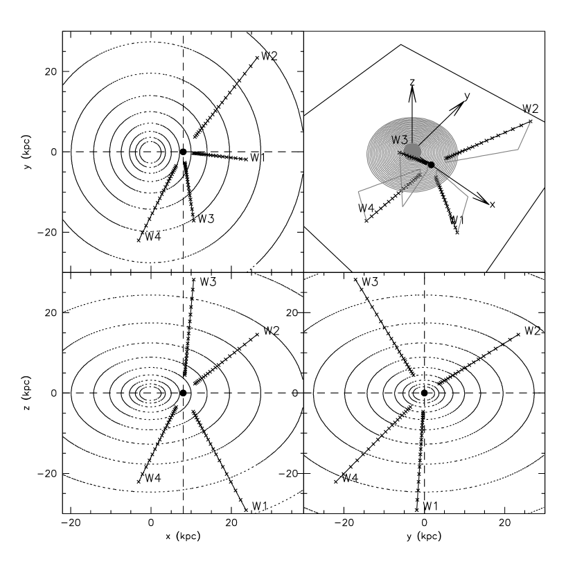
Figure 8: Visualization of the geometry of CFHTLS wide survey beams used in this paper, overplotted on isodensity contours of the J08 halo.

The $x=g-i$ color in Equation 14 is computed from the more accurately measured $g-r$ color using the stellar locus fit from J08 (see their Figure 8). The $[Fe/H]$ is estimated from the $u-g$ and $g-r$ color using the photometric metallicity relation from Bond et al. (2010) (see their Equation A1)

$$[Fe/H]=-13.13+14.09x+28.04y-5.51xy-5.90x^{2}-58.68y^{2}+9.14x^{2}y-20.61xy^{2}+58.20y^{3},$$ (15)

where $x=u-g$ and $y=g-r$. After these cuts, 13692, 7347, 6505 and 6676 stars are left in W1, W2, W3, and W4 beams, respectively.

For each pencil beam, we bin the resulting subset in $\Delta DM=0.2$ mag wide bins in distance modulus, $DM=5\log(D)-5$. We thus obtain the distribution of number counts $\Delta N(l,b,D)$, as a function of distance $D$ for each pencil beam.

We transform the observed counts to density:

$$\rho(l_{i},b_{i},D)=\frac{\Delta{}N(l_{i},b_{i},DM)}{0.2\ln(10)D^{3}\Delta\Omega\Delta{}DM}$$ (16)

where $l_{i},b_{i}$ and $\Delta\Omega_{i}$ are the field centers and area covered by each beam as listed in Table 1, and $\rho(l_{i},b_{i},D)$ is the number density in stars pc^-3. The sightlines sampled by CFHTLS data are shown in Figure 8.

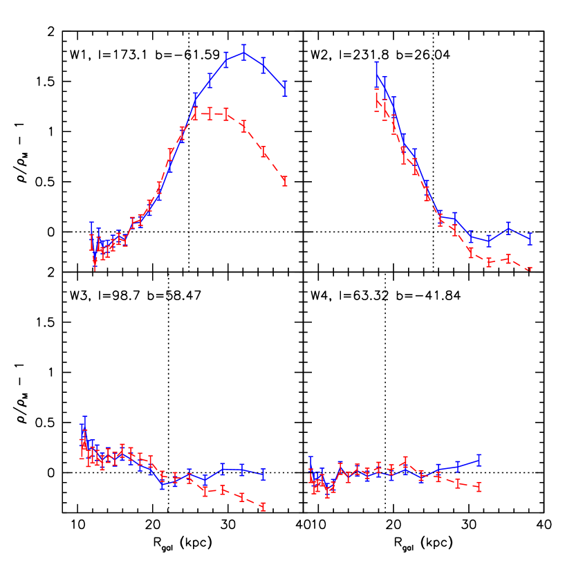
Figure 10: ${\rm Data}/{\rm model}-1$ residuals of the J08 model presented in Figure 9 (dashed line) and of the broken power law model discussed in Section 4 (solid line). The vertical line shows the J08 distance limit. The overdensities in W1 (top left) and W2 (top right) beams are due to the Sagittarius and Monoceros streams, respectively. Beyond $R_{gal}\sim 35$ kpc, the broken power law model provides a much better fit to the data than the single power law J08 model (e.g., the J08 model overpredicts the halo stellar number density by $\gtrsim 50\%$ in W2 and W3 beams at $R_{gal}\gtrsim 35$ kpc).

In panels of Figure 9, we plot the dependence of measured number density on the distance from the Galactic center, $R_{gal}$ for each of the four CFHTLS beams. The measurements are marked by symbols with error bars and connected with a solid line for clarity. Overplotted with a dotted line on each panel is the prediction of the axisymmetric oblate halo model of J08. Plotted as open circles, and connected by red line segments, are samples within $|Z|\leq 5$ kpc of the Galactic plane. As these may be contaminated by disk stars, we leave them out of all further analyses. The residuals of the data for the J08 model are shown in Figure 10.

The density profile observed in W1 beam clearly stands out. While it roughly (within $\sim 20$%) agrees with the predictions of J08 at $R_{gal}\sim 15$ kpc, beyond that radius the observed density begins to exceed the J08 extrapolation, peaking with a factor of $\sim 2$ excess at $R_{gal}\sim 28$ kpc, and dropping towards the end of the observed range ($R_{gal}\sim 35$ kpc). By comparing the location of this overdensity with the best-fit model of the Sagittarius dwarf spheroidal galaxy and its tidal tails (Law & Majewski, 2010), we conclude that the excess is due to the leading and trailing arm of the Sagittarius stream (Ibata, Gilmore & Irwin, 1994; Majewski et al., 2003) crossing the W1 beam. While the distribution and metallicity of stars in this beam may provide useful new constraints for the study of the stream (see Section 6), this (un)fortunate fact makes the majority of W1 data unusable for the study of the smooth halo profile.

Density profiles in W3 and W4 beams agree within $\sim 15$% with the predictions of the J08 halo model in $10<R_{gal}/{\rm kpc}<25$ and $8<R_{gal}/{\rm kpc}<27$ ranges, respectively. The observed agreement is nontrivial. First, the directions observed by these beams do not overlap with the SDSS data used by J08, and therefore test their model in an entirely different part of the halo (especially W4 beam). Second, the CFHTLS data cover a significantly larger distance range than the data used by J08, thus validating the extrapolation to $\sim 10$ kpc greater distances (and an order of magnitude change in stellar number density). And finally, while J08 did use a small ($\sim 300$ deg²) area in the southern Galactic hemisphere to construct their model, their best-fit parameters were largely determined by the $\gtrsim 6000$ deg² of data from the north. The fact that W4 beam ($b=-41\arcdeg.84$) is very well matched by the model puts a constraint to any asymmetries between the northern and southern hemispheres to $\lesssim 15$%, out to distances of at least $R_{gal}\sim 25$ kpc. This conclusion is also supported to distances of $D\lesssim 18$ kpc by the analysis of north versus south SDSS III wide-area imaging (Bonaca, A. et al.(2011), in preparation).

Beyond $R_{gal}\sim 25$ kpc, in both W3 and W4 beams, the J08 model overpredicts the observed counts. In particular, the J08 model overpredicts the density observed in the final two bins of W3 beam by 20% and 40%, respectively. Since we have measured incompleteness to be on the order of $\sim 5$% in almost the entire observed range (see Figure 1), and have made the bins volume-complete, this turnover cannot be a result of observational bias but an indication of a change in halo density profile beyond $R_{gal}\gtrsim 25$ kpc. The overprediction by the model may be even greater since the observed CFHTLS stellar counts are overestimated by 15-20% at the faint end due to the contamination by galaxies, as shown in Figure 1.

The profile exhibited by field W2 is also unusual. As shown in Figure 9, it is significantly steeper than either W3 or W4 profile or the J08 prediction. By itself it is well described by a single $n=-4.5,q=0.65$ power law. This fit, however, is incompatible with observations from the other three directions where a shallower profile closer to $n\sim-2.8$ is strongly preferred. The curious behavior appears to be a combination of two effects: i) the overdensity created by the Monoceros stream at $R_{gal}\lesssim 25$ kpc and ii) the steepening of the halo profile beyond $R_{gal}\sim 30$ kpc.

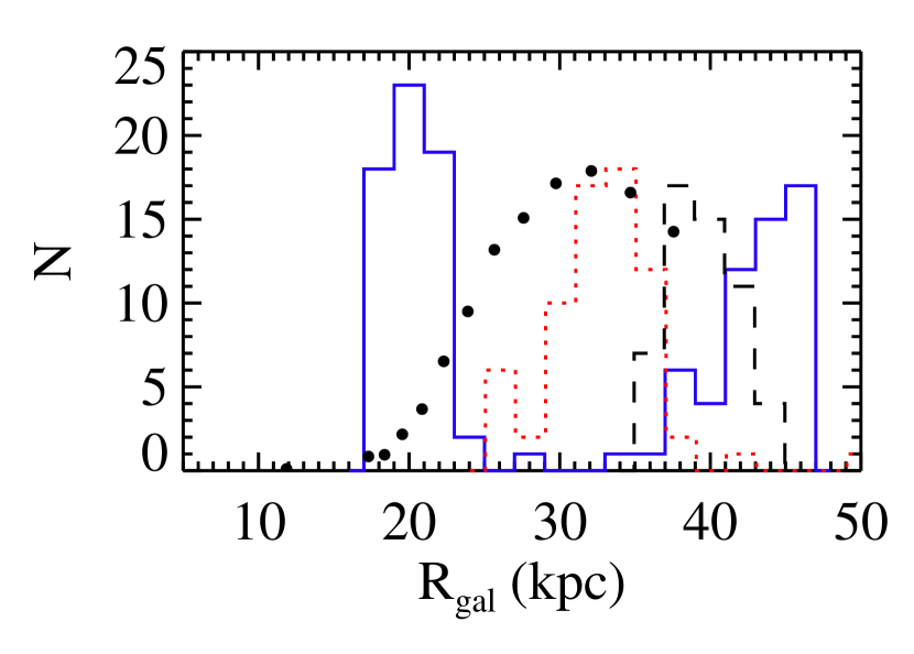
Figure 13: Galactocentric distance (top) and Galactocentric rest-frame radial velocity distribution (bottom) of Sagittarius stream stars in the CFHTLS W1 beam, as predicted by the Law & Majewski (2010) model. The solid and dotted lines denote stars in the first wrap-around leading and trailing tidal streams, respectively. The dashed line represents stars in the leading arm that has wrapped more than $360\arcdeg$ around the Milky Way from Sagittarius (second wrap-around). The solid circles show the observed distribution of Sagittarius tidal stream stars in the W1 beam obtained from ${\rm data}/{\rm model}-1$ residuals of the broken power law model (multiplied by 10). The bottom panel shows that the contribution of different Sagittarius streams to the observed distribution at $R_{gal}\sim 32$ kpc, overplotted in the top panel, can be more easily quantified in the velocity space, since the majority of Sagittarius trailing stream stars are predicted to narrowly distribute around $V_{gsr}<-130$ km s^-1, while the leading stream stars have a much broader velocity distribution and $V_{gsr}>-100$ km s^-1.

The Monoceros stream (Newberg et al., 2002) is present in the general direction of W2 field ($l=232\arcdeg$, $b=26\arcdeg$). For example, in an AAT/WFI survey of the anticenter region, Conn et al. (2007) detect the stream in the $l=220\arcdeg$, $b=15\arcdeg$ direction at $D=11\pm 1.6$ kpc, as well as at $l=240\arcdeg$, $b=10\arcdeg$ with $D=13.8$ kpc. Similarly, J08 are able to trace the stream in SDSS star count maps to $l\sim 230\arcdeg$ and importantly, show that it extends to at least $b\sim 25\arcdeg$ of Galactic latitude where it forms a factor of $\sim 1.5-2$ overdensity with respect to the extrapolation of the smooth stellar background before and after the stream (e.g., as seen in the top left panel of Figure 13 in J08). This is consistent with the factor of $\sim 2$ overdensity observed in W2. Secondly, both of these studies estimate the Galactocentric distance and width of the stream of $R_{gal}\sim 18$ kpc and $\Delta R_{gal}\sim 3-4$ kpc in direction of W2. Given that these characteristics are broadly consistent with the enhancement in the W2 direction for $R_{gal}\lesssim 25$kpc, and having no additional evidence to the contrary, we interpret the observed enhancement as a detection of the Monoceros stream.

4 Detection of a Break in the Halo Density Profile

Taking into account the enhancements due to the Sagittarius and Monoceros streams, a single power law remains an appropriate description of the smooth halo component to Galactocentric distances of $R_{gal}\sim 25-30$ kpc. Beyond this limit, however, the observed profile appears to turn over rather quickly and the model needs to be modified to explain it.

To assess the character of the observed turnover, we fit a series of models of increasing complexity to the observed data. We use $\chi^{2}$ per degree of freedom ($\chi^{2}_{dof}$) as the goodness of fit metric, and search for minima in $\chi^{2}$ hypersurfaces using a Levenberg-Marquardt non-linear solver as implemented by the GNU Scientific Library. To increase the likelihood of finding the true global minimum, we repeat the minimization procedure with 10,000 different initial conditions selected randomly from a plausible range of initial values of each parameter.

We begin by fitting a single J08-type power law to all admissible data points of beams W3 and W4, the first eight data points of W1 beam (those that show no contamination by the Sagittarius stream), and the last six data points of W2 beam (those that we judge are past the influence of the Monoceros stream). We obtain $\rho_{0}=1.7\times 10^{-6}$ pc^-3, $q=0.72$, $n=-2.9$ as the best, but less satisfactory ($\chi^{2}_{dof}=6.8$), fit. The $\rho_{0}$ is the normalization (number of stars per pc³) for the $0.2<g-r<0.3$ color bin we use. For comparison, the fiducial model with J08 parameters shown in Figure 9 has $\chi^{2}_{dof}=9.1$ when fitted to the same data.

We next increase the complexity of the model by allowing for triaxiality of the ellipsoid, parametrized by $w\equiv b/a$ (the ratio of ellipsoid axes):

$$\rho(x,y,z)\propto(x^{2}+\frac{y}{w}^{2}+\frac{z}{q}^{2})^{\frac{n}{2}}$$ (17)

This addition makes practically no difference; the best-fit model changes only slightly ($\rho_{0}=1.7\times 10^{-6}$ pc^-3, $q=0.72$, $n=-2.96$, $w=1.02$) while $\chi^{2}_{dof}$ actually increases (to $\sim 7$) because of the extra degree of freedom.

We continue by permitting the triaxial halo ellipsoid to rotate in the $X-Y$ (Galactic) plane by an angle $\phi$:

$$x^{\prime} = \cos(\phi)\,x-\sin(\phi)\,y$$

$$y^{\prime} = \sin(\phi)\,x+\cos(\phi)\,y$$

$$\rho(x,y,z) \propto (x^{\prime 2}+\frac{y^{\prime}}{w}^{2}+\frac{z}{q}^{2})^{\frac{n}{2}}$$ (18)

This five-parameter model marginally improves the fit ($\chi^{2}_{dof}=6.8$), but converges to parameters $\rho_{0}=1\times 10^{-6}$ pc^-3, $q=1.11$, $n=-3.3$, $w=1.3$, $\phi=230\arcdeg$ that are strongly excluded by prior data (e.g., Chen et al. 2001, J08, and others).

Given the results of this series of experiments, a single power law is unlikely to describe the observed counts: the data require a functional form allowing for a change in the radial profile beyond $R_{gal}\gtrsim 25$ kpc. We therefore attempt a series of simple “broken power law” models, where the density follows one (the “inner”) power law until radius $R_{\rm br}$ is reached, and the other (the “outer” power law) beyond.

We begin with a minimal extension of a single power law model, allowing for a change of the power law index beyond a certain radius $R_{\rm br}$:

$$R_{e} = (x^{2}+y^{2}+\frac{z}{q}^{2})^{\frac{1}{2}}$$

$$\rho(x,y,z) \propto \left\{\begin{array}[]{c}(R_{e})^{n_{\rm inner}},\;\;\;\;\;\;\;R_{e}<R_{\rm br}\\ (R_{e})^{n_{\rm outer}},\;\;\;\;\;\;\;R_{e}>R_{\rm br}\\ \end{array}\right.$$ (21)

Note that, as the ellipsoid is allowed to be oblate or prolate, the break radius $R_{\rm br}$ is only equal to the physical Galactocentric radius $R_{gal}$ on the $x$ axis (along the line connecting the Galactic center and the Sun). In the vertical direction, the physical radius corresponding to $R_{\rm br}$ is reduced by a factor of $q^{-1}$.

The above model, with five free parameters, produces a significantly better fit to the data ($\chi^{2}_{dof}=3.9$). The best-fit parameters for the inner power law, $\rho_{0}=(1.45\pm 0.05)\times 10^{-6}$ pc^-3, $q=0.70\pm 0.01$, $n_{\rm inner}=-2.62\pm 0.04$, $R_{\rm br}=27.8\pm 0.8$ kpc, $n_{\rm outer}=-3.8\pm 0.1$ are in excellent agreement with the J08 model, while beyond $R_{\rm br}=27.8$ kpc the best-fit profile becomes steeper than the J08 model.

As shown in Figure 10, the observed profiles are better fit by the broken power law than by the J08 model, excluding regions with known tidal streams. A fit that entirely excludes W1 and W2 fields (not just the regions with known tidal streams) does not strongly constrain the broken power law model. In this fit, the normalization $\rho_{0}$ has high ($\sim 50\%$) fractional uncertainty and strongly correlates with oblateness $q$ and break radius $R_{\rm br}$ (correlation coefficient is $\sim 1$). This strong correlation is caused by similar positions of W3 and W4 beams in $x-z$ and $y-z$ planes with respect to the Galactic plane (see Figure 8). In comparison, our best-fit profile that uses all four beams while excluding regions with known tidal streams shows much weaker correlation between $\rho_{0}$, $q$, and $R_{\rm br}$ ($\sim 0.4$).

The inner parts of the W3 field in our best-fit model do show a systematic underestimate of the counts by the model on the order of $\sim 15$% (at an approximately $1\sigma$-$2\sigma$ level), while the opposite occurs in inner parts of the W1 field. These lines of sight point toward high latitudes in the northern and southern Galactic hemispheres, and the observed difference may be a signature of slight north-south asymmetry of halo star counts recently seen in SDSS III data (Bonaca, A. et al.(2011), in preparation).

To further assess the robustness of the detected break, we examined two more variants of the model: the first, where we allowed the outer halo to have an oblateness parameter $q$ different from that of the inner halo, and the second, where we fixed the parameters of the inner halo to J08 values, and allowed only those of the outer halo to vary. Both cases resulted in a similar value of $\chi^{2}_{dof}$, as well as similar break radii ($R_{\rm br}\sim 28$ kpc) and outer power law indices ($n_{\rm outer}\sim-3.8$). Importantly, the model with varying $q_{\rm inner}$ and $q_{\rm outer}$ produced best-fit values of $0.71$ and $0.69$ for the two, respectively, indicating that there is no evidence for a change in oblateness of the halo across the range of distances examined.

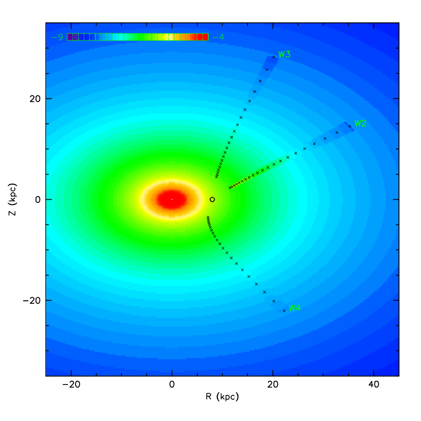
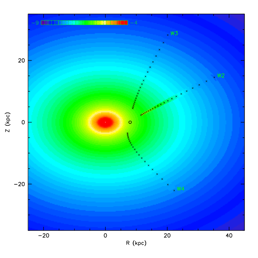
Figure 11: $R-Z$ plane visualization of the J08 power law halo model (left) and the broken power law model presented in this paper (right). The color encodes the logarithm of the number density of halo stars (stars pc^-3) predicted by the model. Overplotted are the densities derived from the analysis of CFHTLS data (beams W2, W3 and W4) presented in this paper (W1 beam is not shown because of the strong contamination by the Sagittarius stream). Note the marked improvement in data-model agreement for the broken power law model.

Based on the above analysis, we conclude that the detection of steepening of the halo density power law is robust. To explain the CFHTLS data, the power law index needs to change from $n_{\rm inner}=-2.62$ to $n_{\rm outer}=-3.8$ around $R_{\rm br}\sim 28$ kpc. An R$-$Z plane visualization of the J08 power-law halo model and the broken power-law model presented in this paper is shown in Figure 11.

We also fit Einasto’s model (Einasto, 1965) to our data to allow easy comparison with density profiles obtained from $N$-body simulations (Navarro et al., 2004; Diemand, Moore & Stadel, 2004; Merritt et al., 2005; Graham et al., 2006). The best-fit parameters for the Einasto’s model are $n=2.2\pm 0.2$, $R_{e}=22.2\pm 0.4$ kpc, $\rho_{0}=1.06\pm 0.05$ stars pc^-3, and $q=0.70\pm 0.01$ with $chi^{2}_{pdf}=4.25$.

Due to contamination by galaxies at the faint end (see Figure 1), the $n_{\rm outer}=-3.8\pm 0.1$ power law index given above is likely somewhat shallower than what it should be. To estimate by how much $n_{\rm outer}$ is shallower due to contamination by galaxies, we determine $f(r)=[1-contamination(r)]/completeness(r)$ for each star, where $r$ is a star’s $r$ band magnitude, and $completeness(r)$ and $contamination(r)$ are the solid and dashed lines from Figure 1, respectively. We sum $f(r)$ values in distance modulus bins and use them instead of raw number counts when fitting the model. With this approach, a star located in a distance modulus bin with higher galaxy contamination will contribute a value smaller than one towards the total count in that bin. Finally, we find that $n_{\rm outer}$ decreases by 0.1 to $n_{\rm outer}=-3.9$, which is still within the uncertainty of $n_{\rm outer}=-3.8\pm 0.1$ determined previously.

5 Metallicity Distribution in the Halo and its Impact on the Best-fit Model

In addition to stellar number density distribution, the metallicity distribution can also provide strong constraints for halo formation models. Thanks to CFHTLS $u$ band data, it is possible to compute photometric metallicity using a method developed by Ivezić et al. (2008a). Furthermore, the absolute magnitude of a star, and hence its distance, depend on the star’s metallicity (Equation 14) and thus it is important to study systematic errors in best-fit model parameters as a function of metallicity distribution.

Figure 12 shows the median halo metallicity in four CFHTLS beams as a function of distance from the Galactic center, $R_{gal}$. In the two beams where significant substructure is not detected (W3 and W4 beams), the median metallicity is independent of distance and averages to $[Fe/H]\sim-1.5$ dex with a range of 0.1 dex. This average value is consistent with the median halo metallicity measured by Ivezić et al. (2008a) using SDSS F- and G-type main sequence stars, and the range is consistent with the systematic uncertainty inherent to this photometric metallicity method ($\sim 0.1$ dex, Ivezić et al. 2008a).

The average metallicity in the W1 beam is also independent of distance and averages $[Fe/H]\sim-1.5$ dex. This trend is probably a coincidence since the Sagittarius tidal stream passes through the beam and the stream’s metallicity is not required to be $[Fe/H]\sim-1.5$ dex everywhere. On the contrary, models and observations (Chou et al. 2007; Sesar et al. 2010; Law & Majewski 2010 and references therein) suggest that the metallicity exhibits a gradient along the Sagittarius tidal stream — we simply happen to observe the stream where its metallicity is $[Fe/H]\sim-1.5$ dex.

The metallicity in the W2 beam is a bit higher ($[Fe/H]\sim-1.3$ dex) than in other beams, even at large Galactocentric distances ($R_{gal}>28$ kpc) where, according to Figure 10 (top right panel), the contribution of the Monoceros stream stars should be small. Since the Ivezić et al. (2008a) photometric metallicity method depends on accurate $u$ band photometry, anything affecting $u$ band measurements will also affect the photometric metallicity estimate. As discussed in Section 2.4, the $u$ band measurements synthesized from CFHTLS data may be impacted by some calibration issues in this beam, so these issues are likely responsible for the apparently higher metallicity in the W2 beam (a $+0.05$ mag systematic offset in the $u$ band will increase the metallicity by 0.2 dex).

Our observation that the halo metallicity is independent of Galactocentric distance goes contrary to Carollo et al. (2007) and de Jong et al. (2010) (hereafter deJ10) results who conclude that the halo metallicity changes from $[Fe/H]\sim-1.6$ dex to $[Fe/H]\sim-2.2$ dex at $R_{gal}\sim 15$ kpc. To see how our best-fit model varies when the metallicity changes from $[Fe/H]\sim-1.6$ dex for $R_{gal}\lesssim 15$ kpc to $[Fe/H]\sim-2.2$ dex beyond $R_{gal}\sim 15$ kpc, we iteratively modify the metallicity distribution in CFHTLS beams to reflect the metallicity distributions shown in deJ10 Figure 7 (right, hereafter $[Fe/H]_{deJ10}(D)$). New metallicities are assigned to CFHT stars by interpolating $[Fe/H]$ from $[Fe/H]_{deJ10}(D)$ using initial heliocentric distances, $D$ (calculated from Equations 14 and 15). Heliocentric distances are then recalculated using new metallicity values, and the metallicities are again interpolated from $[Fe/H]_{deJ10}(D)$). This process is repeated (about 2-3 times) until the fractional difference between distances in consecutive steps dips below 0.15 (fractional distance uncertainty for main sequence stars is $\sim 15\%$; Sesar, Ivezić & Jurić 2008). The broken power law model is fit to modified data once the convergence is achieved.

The best-fit model parameters obtained for deJ10-like metallicity distribution are listed in Table 4. In addition, Table 4 also lists best-fit model parameters obtained for constant metallicity distributions (i.e., all stars are assumed to have fixed metallicity) and for the best-fit model presented in Section 4. Within a range of plausible metallicity distributions, the best-fit model parameters do not seem to vary greatly and average around $q\sim 0.7$, $n_{inner}\sim-2.4$, $n_{outer}\sim-3.8$, and $R_{br}\sim 25$ kpc.

6 Conclusions and Discussion

We have recalibrated CFHTLS “wide” survey $u^{*}g^{\prime}r^{\prime}i^{\prime}i^{\prime}_{2}$ observations and transformed them to the SDSS $ugri$ photometric system. Using a series of tests, we demonstrated that synthesized $ugri$ observations, when compared to SDSS observations, show no dependence on color or magnitude. The only exception to this are the $u$ band observations synthesized from CFHTLS W2 field $u^{*}$ band observations, which show a slight linear dependence on the $u-g$ color. Median photometric error in synthesized $ugri$ photometry is $\sim 0.03$ mag at the bright end and $\sim 0.1$ mag at $\sim 22.5$ mag.

By obtaining the synthesized $ugri$ photometry from CFHTLS observations, we were able to use the photometric parallax and metallicity relations which allowed us to study the spatial and metallicity distribution of near-turnoff main sequence stars in the Galactic halo to heliocentric distances of $\sim 35$ kpc. We find that the halo number density profile becomes steeper at Galactocentric distances greater than $R_{gal}\sim 28$ kpc, with the power law index changing from $n_{inner}=-2.62\pm 0.04$ to $n_{outer}=-3.8\pm 0.1$. While the best-fit model parameters do change slightly depending on the adopted metallicity distribution (see Table 4), we find that a broken power law model is required for a good fit to the data. We also find that the best-fit $R_{br}$ value cannot be smaller than $R_{br}=22$ kpc even for the most extreme assumptions about the halo metallicity distribution (i.e., constant metallicity at $[Fe/H]=-2.0$ dex from 5 to 35 kpc).

This study provides further evidence for the steepening of the halo density profile previously detected by Sesar et al. (2010) using main sequence and RR Lyrae stars from the SDSS stripe 82, and by Keller et al. (2008) using RR Lyrae stars from the SEKBO survey. This result is consistent with predictions of galaxy formation simulations which find a steepening of the density profile beyond $\sim 30$ kpc (Bullock & Johnston, 2005; De Lucia & Helmi, 2008; Zolotov et al., 2009).

We see no evidence of change in halo metallicity within the range of probed distances. The halo metallicity ranges between $[Fe/H]\sim-1.4$ dex and $[Fe/H]\sim-1.6$ dex, and averages at $[Fe/H]\sim-1.5$ dex. This result runs contrary to Carollo et al. (2007) and de Jong et al. (2010) studies which report a metallicity of $[Fe/H]\sim-1.6$ dex within $R_{gal}\lesssim 15$ kpc, and $[Fe/H]\sim-2.2$ dex beyond. Only the in situ spectroscopic metallicities of distant main sequence stars may provide a definitive answer to this discrepancy. With the sky density of near-MSTO stars at high Galactic latitudes of about 100 stars deg², the multi-object capability over a wide field of view would be well matched to such a program.

While the total sky coverage of the four CFHTLS beams is slightly smaller than that of SDSS stripe 82 (220 deg² versus 300 deg²), the CFHTLS beams provide a much stronger constraint on the oblateness ($Z$ to $R$ semi-major axis ratio) of the stellar halo because they probe very different Galactic lines of sight. We find the oblateness to be $q=0.70\pm 0.01$ and see no evidence of change across the range of probed distances ($5<R_{gal}/{\rm kpc}<35$). This result is quite consistent with the oblateness of the dark matter halo, $q_{DM}=0.72$, obtained by Law & Majewski (2010) using the positions and kinematics of Sagittarius stream stars. However, we find the minor axis of the stellar halo to be aligned with the spin vector of the Milky Way, while Law & Majewski (2010) find the minor axis of the dark matter halo to be perpendicular to the spin vector of the Milky Way.

We have detected the Sagittarius and Monoceros streams as excesses of stars in CFHTLS W1 and W2 fields, respectively. These detections provide new constraints on models of these streams. For example, the Law & Majewski (2010) model of the Sagittarius dwarf spheroidal galaxy predicts positions and velocities of Sagittarius stream stars in the CFHTLS W1 beam (Figure 13). The spatial distribution of Sagittarius stars is predicted to be bimodal, with a narrow peak at $R_{gal}\sim 20$ kpc, and a broader peak at $R_{gal}\sim 35$ kpc. The observed distribution of Sagittarius stars in this region, overplotted in Figure 13 (top panel), has only one peak at $R_{gal}\sim 35$ kpc. Unfortunately, we do not have radial velocity measurements in this region, and cannot quantify contributions of particular streams (leading and trailing) to this peak. Multi-epoch surveys, such as the Palomar Transient Factory (PTF; Law et al. 2009) and LSST, will enable robust identification of bright tracers such as RR Lyrae stars, which can be used to map the velocity structure in this region. The resulting improvement in models of these streams may then help to further constrain the shape, orientation, and the mass of the Galactic dark matter halo.

Table 1: Overview of the CFHTLS Wide fields

CFHTLS Field Name	$\alpha^{a}$ $(deg)$	$\delta^{a}$ $(deg)$	lb $(deg)$	bb $(deg)$	Sky Coverage $(deg^{2})$
W1	34.5	-7.0	173.12	-61.59	72
W2	134.5	-3.3	231.78	26.04	25
W3	214.4	54.5	98.70	58.47	49
W4	333.3	1.3	63.32	-41.84	25

Table 2: $\Delta_{f}^{abs}$ Values for CFHTLS “Wide” Fields

			$\Delta_{f}^{abs}$
CFHT Band	SDSS Color Range	C	W1	W2	W3	W4
$u^{*}$	$1.1<u-g<1.4$	-0.155	0.087	0.099	0.098	0.097
$g^{\prime}$	$0.3<g-r<1.2$	-0.161	-0.017	-0.044	-0.037	-0.043
$r^{\prime}$	$0.4<g-r<1.2$	-0.018	-0.030	-0.019	-0.027	-0.027
$i^{\prime}$	$0.3<r-i<1.0$	-0.081	-0.020	-0.015	-0.022	-0.030
$i^{\prime}_{2}$	$0.3<r-i<1.0$	0.020	0	n/a	n/a	0

Table 3: $\Delta_{j,f}^{total}$ Values for the CFHTLS W1$-$W4 fields

Pointinga	$u^{*}$	$g^{\prime}$	$r^{\prime}$	$i^{\prime}$
W1+0-2	0.106	-0.034	-0.034	-0.048
W1+0-3	0.105	-0.030	-0.028	-0.040
W1+0-4*	0.077	-0.023	-0.026	0.001

Note. — This table is available in its entirety in machine-readable form in the online journal. A portion is shown here for guidance regarding its form and content.

Table 4: Best-fit Model Parameters and their Uncertainties

Adopted Metallicity	$\rho_{0}^{a}$ ($10^{-6}$ pc-3)	qb	$n_{inner}$	$R_{br}$ (kpc)	$n_{outer}$	$\chi^{2}_{dof}$c
Equation 15d	$1.45\pm 0.05$	$0.70\pm 0.01$	$-2.62\pm 0.04$	$27.8\pm 0.8$	$-3.8\pm 0.1$	3.9
de Jong et al. (2010)e	$1.25\pm 0.04$	$0.76\pm 0.01$	$-2.32\pm 0.04$	$24.3\pm 0.3$	$-6.4\pm 0.1$	9.6
$[Fe/H]=-1.0^{f}$	$1.02\pm 0.04$	$0.72\pm 0.01$	$-2.32\pm 0.04$	$28.5\pm 0.6$	$-3.8\pm 0.1$	5.7
$[Fe/H]=-1.5^{f}$	$1.32\pm 0.05$	$0.73\pm 0.01$	$-2.47\pm 0.05$	$24.8\pm 0.7$	$-3.86\pm 0.08$	4.4
$[Fe/H]=-2.0^{f}$	$1.51\pm 0.06$	$0.72\pm 0.01$	$-2.50\pm 0.06$	$22.1\pm 0.6$	$-3.81\pm 0.06$	4.6

Figure 1: The fraction of SDSS stars identified as stars in CFHTLS data (completeness, solid line) and the fraction of CFHTLS stars identified as galaxies by the SDSS (contamination, dashed line) as a function of CFHTLS $r^{\prime}$ magnitude (not corrected for ISM extinction). Using this plot, we estimate that the observed number counts will be underestimated by about $5\%$ for $r^{\prime}<21$ and overestimated by about 15%$-$20% at the faint end ($r^{\prime}\sim 22.5$).

Figure 12: Median photometric metallicity (symbols with error bars) measured in four CFHTLS wide survey beams as a function of distance from the Galactic center, $R_{gal}$. The error bars show error in the median and the error bar at (6.5, -1.5) shows the systematic uncertainty in the adopted photometric metallicity method ($\sim 0.1$ dex, Ivezić et al. 2008a). Within $R_{gal}\sim 30$ kpc, the median metallicity is independent of distance and ranges from $-1.4<[Fe/H]<-1.6$. The change in metallicity at $R_{gal}\sim 15$ kpc, reported by Carollo et al. (2007) and de Jong et al. (2010), is not evident. Apparently higher metallicity in the W2 beam ($[Fe/H]\sim-1.3$ dex) may be due to $u$ band calibration issues (see the text for a discussion).

References

- Abazajian et al. (2009) Abazajian, K. N. et al. 2009, ApJS, 182, 543
- Bertin & Arnouts (1996) Bertin, E. & Arnouts, S. 1996, A&A, 117, 393
- Bond et al. (2010) Bond, N. A. et al. 2010, ApJ, 716, 1
- Boulade et al. (2003) Boulade, O. et al. 2003, Proc. SPIE, 4841, 72
- Bullock & Johnston (2005) Bullock, J. S. & Johnston, K. V. 2005, ApJ, 635, 931
- Carollo et al. (2007) Carollo, D. et al. 2007, Nature, 450, 1020
- Carollo et al. (2010) Carollo, D. et al. 2010, ApJ, 712, 692
- Chen et al. (2001) Chen, B. et al. 2001, ApJ, 553, 184
- Chou et al. (2007) Chou, M.-Y. et al. 2007, ApJ, 670, 346
- Conn et al. (2007) Conn, B. C. et al. 2007, MNRAS, 376, 939
- de Jong et al. (2010) de Jong, J. T. A., Yanny, B., Rix, H.-W., Dolphin, A. E., Martin, N. F., & Beers, T. C. 2010, ApJ, 714, 663
- De Lucia & Helmi (2008) De Lucia, G. & Helmi, A. 2008, MNRAS, 391, 14
- Diemand, Moore & Stadel (2004) Diemand, J., Moore, & B. Stadel, J. 2004, MNRAS, 353, 624
- Einasto (1965) Einasto, J. 1965, Trudy Inst. Astrofiz. Alma-Ata, 5, 87
- Fukugita et al. (1996) Fukugita, M., Ichikawa, T., Gunn, J. E., Doi, M., Shimasaku, K., & Schneider, D. P. 1996, AJ, 111, 1748
- Goranova et al. (2009) Goranova, Y. et al. 2009, http://terapix.iap.fr/cplt/T0006-doc.pdf
- Graham et al. (2006) Graham, A. W., Merritt, D., Moore, B., Diemand, J., & Terzić, B. 2006, AJ, 132, 2711
- Gwyn (2008) Gwyn, S. D. J. 2008, PASP, 120, 212
- Ibata, Gilmore & Irwin (1994) Ibata, R. A., Gilmore, G. & Irwin, M. J. 1994, Nature, 370, 194
- Ivezić et al. (2004) Ivezić, Ž. et al. 2004, Astronomische Nachrichten, 325, 583
- Ivezić et al. (2008a) Ivezić, Ž. et al. 2008a, ApJ, 684, 287
- Ivezić et al. (2008b) Ivezić, Ž. et al. 2008b, arXiv:0805.2366
- Jurić et al. (2008) Jurić, M. et al. 2008, ApJ, 673, 864, (J08)
- Kaiser et al. (2002) Kaiser, N. et al. 2002, Proc. SPIE, 4836, 154
- Keller et al. (2008) Keller, S. C., Murphy, S., Prior, S., Da Costa, G., & Schmidt, B. 2008, ApJ, 678, 851
- Law et al. (2009) Law, N. M. et al. 2009, PASP, 121, 1395
- Law & Majewski (2010) Law, D. R. & Majewski, S. R. 2010, ApJ, 714, 229
- Lin et al. (2009) Lin, H., Flaugher, B. & The Dark Energy Survey Collaboration 2009, BAAS, 41, 669
- LSST Science Book (2009) LSST Science Collaborations and LSST Project 2009, LSST Science Book, Version 2.0, arXiv:0912.0201, http://www.lsst.org/lsst/scibook
- Lupton et al. (2002) Lupton, R. H., Ivezić, Ž, Gunn, J. E., Knapp, G., Strauss, M. A., & Yasuda, N. 2002, Proc. SPIE, 4836, 350
- Magnier & Cuillandre (2004) Magnier, E. A. & Cuillandre, J. C. 2004, PASP, 116, 449
- Majewski et al. (2003) Majewski, S. R., Skrutskie, M. F., Weinberg, M. D., & Ostheimer, J. C. 2003, ApJ, 599, 1082
- Merritt et al. (2005) Merritt, D., Navarro, J. F., Ludlow, A., & Jenkins, A. 2005, ApJ, 624, 85
- Navarro et al. (2004) Navarro, J. F. et al. 2004, MNRAS, 349, 1039
- Newberg et al. (2002) Newberg, H. J. et al. 2002, ApJ, 569, 245
- Padmanabhan et al. (2008) Padmanabhan, N. et al. 2008, ApJ, 674, 1217
- Schlegel, Finkbeiner & Davis (1998) Schlegel, D., Finkbeiner, D. P. & Davis, M. 1998, ApJ500, 525
- Schultheis et al. (2006) Schultheis, M., Robin, A. C., Reylé, C., McCracken, H. J., Bertin, E., Mellier, Y., & Le Fèvre, O. 2006, A&A, 447, 185
- Sesar, Ivezić & Jurić (2008) Sesar, B., Ivezić, Ž. & Jurić, M. 2008, ApJ, 689, 1244
- Sesar et al. (2010) Sesar, B. et al. 2007, ApJ, 708, 717
- York et al. (2000) York, D. G. et al. 2000, AJ, 120, 1579
- Zolotov et al. (2009) Zolotov, A., Willman, B., Brooks, A. M., Governato, F., Brook, C. B., Hogg, D. W., Quinn, T., & Stinson, G. 2009, ApJ, 702, 1058