TRANSPORT AND SPECTRA IN THE HALF-FILLED HUBBARD MODEL: A DYNAMICAL MEAN FIELD STUDY

Abstract

We study the issues of scaling and universality in spectral and transport properties of the infinite dimensional particle–hole symmetric (half–filled) Hubbard model within dynamical mean field theory. One of the simplest and extensively used impurity solvers, namely the iterated perturbation theory approach is reformulated to avoid problems such as analytic continuation of Matsubara frequency quantities or calculating multi-dimensional integrals, while taking full account of the very sharp structures in the Green’s functions that arise close to the Mott transitions and in the Mott insulator regime. We demonstrate its viability for the half-filled Hubbard model. Previous known results are reproduced within the present approach. The universal behavior of the spectral functions in the Fermi liquid regime is emphasized, and adiabatic continuity to the non-interacting limit is demonstrated. The dc resistivity in the metallic regime is known to be a non-monotonic function of temperature with a ‘coherence peak’. This feature is shown to be a universal feature occurring at a temperature roughly equal to the low energy scale of the system. A comparison to pressure dependent dc resistivity experiments on Selenium doped NiS₂ yields qualitatively good agreement. Resistivity hysteresis across the Mott transition is shown to be described qualitatively within the present framework. A direct comparison of the thermal hysteresis observed in V₂O₃ with our theoretical results yields a value of the hopping integral, which we find to be in the range estimated through first-principle methods. Finally, a systematic study of optical conductivity is carried out and the changes in absorption as a result of varying interaction strength and temperature are identified.

Keywords: Hubbard model; dynamical mean field theory; iterated perturbation theory; optical conductivity; hysteresis

PACS: 71.10.Fd, 71.10.-w, 71.30.+h, 71.27.+a, 78.20.-e

1 Introduction

The Hubbard model (HM) [1, 2, 3, 4] has become one of the central paradigms in theories for strongly correlated electron systems. For systems ranging from ultracold gases [5], transition metal oxides [6, 7], high temperature superconductors [8, 9], and even graphene [10, 11], the HM has been employed in various guises. Thus, the importance of developing an understanding of this model cannot be overstated. The theoretical techniques that have been employed in an attempt to solve this model are diverse, e.g. Hatree-Fock approximation [12, 13, 14], Hubbard’s Green’s function approximations [15, 16], variational wave function method [4, 17], slave Boson approach [18], etc. However, to date the general HM remains unsolved except for the one-dimensional case [19]. A lot of progress has been made in recent years in this direction through the dynamical mean field theory (DMFT) [20, 21], where the lattice model is mapped onto an effective single impurity model with a self-consistently determined hybridization. Within the DMFT context, a greater interest is being devoted towards the inifinite dimensional HM since the mapping becomes exact in the limit and simplifies many major issues of many-body approaches. Although the lattice problem reduces to that of an impurity problem embedded in a non-interacting bath, the problem remains amenable to a host of techniques such as non-crossing approximation (NCA) [22], quantum Monte Carlo(QMC) [9, 23, 21], numerical renormalization group (NRG) [24], exact diagonalization (ED) [25], iterated perturbation theory (IPT) [26, 21, 27, 28], local moment approach (LMA) [29, 30], etc, that have been developed to solve the impurity problem. IPT is a particularly simple diagrammatic perturbation theory based approach that has been extensively used to study not only the impurity problem, but also a host of other lattice based models such as the HM and the periodic Anderson model (PAM) [31]. It is known to yield qualitatively good results, such as the Mott metal-insulator transition, heavy fermion behavior etc. However, since it is perturbative by construction, IPT does not do as well in quantitative terms. The half-filled HM, has likewise, been a very intensively studied model, as a description of the Mott MIT, and IPT has been very successful in elucidating quite a few conceptual issues [27, 28]. Nevertheless, we observe a few important deficiencies in the present implementations of IPT, specifically for the half-filled HM. IPT, as implemented generally, calculates Matsubara frequency Green’s functions and self-energies. The procedure of analytic continuation, required to obtain real frequency quantities, is known to be a numerically difficult problem, which is conventionally treated by Padé approximation or the maximum entropy method [32, 21]. The direct real frequency implementation takes two routes – in the first, one has to solve multi-dimensional integrals, which is computationally expensive; the other route employs Fast Fourier transforms, which has the disadvantage that the frequency grid is necessarily uniform, and thus cannot sample the very sharp structures arising in the Green’s functions in the parameter region proximal to the Mott transition as well as in the Mott insulator regime. This leads to problems in convergence of the DMFT iterations. In a very recent study, an ad-hoc way of dealing with the sharp structures was implemented through the addition of a small constant imaginary part added to the real frequency [33]. This method broadens the poles of the Green’s functions and lets one handle the sharp structures numerically. However, it has the disadvantage that it leads to spurious spectral features, e.g. the insulating phase does not exhibit a clear gap.

In this work, we introduce an alternative real frequency implementation that overcomes the above limitations, and hence, lets one study the properties of interest such as spectral functions etc directly on the real axis with an adaptive non-uniform grid. In order to solve the DMFT self-consistency equations we start with an initial guess for the self-energy (typically the Hatree-Fock) whereas the host Green’s function is guessed initially in common practice. We benchmark our results against known IPT results calculated through analytic continuation of the Matsubara frequency Green’s functions. We find excellent agreement. Issues of universality and scaling of spectral functions and transport quantities are emphasized. The paper is organized as follows: The next section details the model and the reformulation of IPT. The numerical implementation details are also discussed. Section 3 comprises our theoretical results, discussion and comparison to experiments. We present our conclusions in section 4.

2 Methods and Formalism

The single-band HM in standard notation is given by

$$\hat{H}=-\sum_{<ij>,\sigma}t_{ij}(c_{i\sigma}^{\dagger}c_{j\sigma}^{\phantom{d}}+\textrm{h}.c.)+\epsilon_{d}\sum_{i\sigma}c_{i\sigma}^{\dagger}c_{i\sigma}^{\phantom{d}}+U\sum_{i}n_{i\uparrow}n_{i\downarrow}$$ (1)

where $t_{ij}$ is the amplitude of hopping of electrons from site-$i$ to site-$j$ , $\epsilon_{d}$ is the electron’s orbital energy and $U$ is the on-site Coulomb repulsion. The operator $c_{i\sigma}$ ($c_{i\sigma}^{\dagger}$) annihilates (creates) an electron of spin $\sigma$ at site $i$. In the limit of infinite dimensions $(d\rightarrow\infty)$, the hopping parameter is scaled as $t=t_{\ast}/\sqrt{z}$ where $z$ is the coordination number of the lattice. In this work, we choose to work with the hypercubic lattice (HCL) for which the non-interacting ($U=0$) density of states is an unbounded gaussian, i.e.

$$D_{0}(\epsilon)=\frac{1}{\sqrt{\pi}t_{\ast}}\exp(-\epsilon^{2}/{t_{\ast}^{2}})$$ (2)

The major simplification within DMFT, which is exact in $d=\infty$, is that the self-energy [20] and vertex function [34] become momentum independent or spatially local. The local, retarded Green’s function in the paramagnetic case is given by

$$G(\omega)=\sum_{\bf{k}}\frac{1}{\omega^{+}-\epsilon_{k}-\epsilon_{d}-\Sigma(\omega)}$$ (3)

where $\omega^{+}=\omega+i\eta$, $\eta\rightarrow 0^{+}$ and $\Sigma(\omega)$ is the real-frequency self-energy. The $\bf{k}$ sum may be transformed to a density of states integral and thus may be written as

$$G(\omega)={\mathcal{H}}[\gamma(\omega)]$$ (4)

where ${\mathcal{H}}[z]=\int d\epsilon\,D_{0}(\epsilon)/(z-\epsilon)$ is the Hilbert transform of $z$ with respect to $D_{0}(\epsilon)$ and $\gamma(\omega)=\omega^{+}-\epsilon_{d}-\Sigma(\omega)$. Since a lattice model can be mapped onto an impurity model within DMFT with the self-consistency condition that the impurity self-energy is the same as the lattice self-energy, one can find the host or medium Green’s function ${\mathcal{G}}(\omega)$ for the impurity through the Dyson equation

$${\mathcal{G}}^{-1}(\omega)=G^{-1}(\omega)+\Sigma(\omega)$$ (5)

Solution of the impurity model in terms of $\mathcal{G}(\omega)$ would then yield a new $\Sigma(\omega)$ which when put back in Eq. (4) gives $G(\omega)$. Thus, given an impurity solver technique, one can self-consistently solve for the Green’s functions, and hence the self-energy. Since the vertex function is also momentum independent within DMFT, the calculation of conductivity through the current-current correlation function involves only single-particle quantities. Thus the optical conductivity may be calculated by using the following expression obtained from the Kubo formula [35].

$$\sigma(\omega)=\frac{\sigma_{0}}{2\pi^{2}}\rm{Re}\int_{-\infty}^{\infty}d\omega^{\prime}\,\frac{n_{F}(\omega^{\prime})-n_{F}(\omega+\omega^{\prime})}{\omega}\times$$

$$\bigg{[}\frac{G^{\ast}(\omega^{\prime})-G(\omega+\omega^{\prime})}{\gamma(\omega+\omega^{\prime})-\gamma^{\ast}(\omega^{\prime})}-\frac{G(\omega^{\prime})-G(\omega+\omega^{\prime})}{\gamma(\omega+\omega^{\prime})-\gamma(\omega^{\prime})}\bigg{]}$$ (6)

where $\sigma_{0}=4\pi e^{2}t^{2}a^{2}n/\hbar$ for lattice constant $a$, electronic charge $e$, and electron density $n$. As $\omega\rightarrow 0$ we obtain the DC conductivity :

$$\sigma_{DC}=\frac{\sigma_{0}}{2\pi^{2}}{\rm Re}\int^{\infty}_{-\infty}d\omega\,\left(-\frac{dn_{F}}{d\omega}\right)\left[\frac{\pi D(\omega)}{\rm{Im}\gamma(\omega)}+2(1-\gamma(\omega)G(\omega)\right]$$ (7)

where $D(\omega)=-\frac{1}{\pi}\mathrm{Im}G(\omega)$ is the spectral function of the retarded Green’s function $G(\omega)$ and $n_{F}(\omega)=(e^{\beta\omega}+1)^{-1}$ is the Fermi function ($\beta=1/(k_{B}T)$).

As mentioned earlier, the full solution of DMFT problem requires an impurity solver technique. In this paper, we have chosen IPT for solving the self-consistent impurity problem. IPT does have a few drawbacks. It is based on a simple truncation of the diagrammatic perturbation theory in $U$ to second order around the Hartree mean field solution. Thus it needs to be benchmarked for every new problem. For the same reason, it is unable to capture exponentially small energy scales. Nevertheless, the reason for this choice is that IPT is technically one of the simplest approaches that can capture the Mott transition physics in a qualitatively correct manner. IPT has been extensively employed by various groups to study the HM [27, 28, 21] and PAM [36, 37, 38, 39]. However, the previous implementations suffer from the problems mentioned in the introduction section.

We now describe IPT and our implementation of it briefly. The ansatz for the dynamical part of the self-energy (apart from the static Hartree term) within IPT is just the second order term of the perturbative expansion in $U$ about the Hartree limit, i.e.

$$\Sigma_{2}(\omega)=\lim_{i\omega\rightarrow\omega^{+}}\frac{U^{2}}{\beta^{2}}\sum_{m,p}{\mathcal{G}}(i\omega+i\nu_{m}){\mathcal{G}}(i\omega_{p}+i\nu_{m}){\mathcal{G}}(i\omega_{p})$$ (8)

where $i\omega$ and $i\nu$ denote odd and even Matsubara frequencies respectively. Using the spectral representation $\mathcal{G}(i\omega_{n})=\displaystyle\int_{-\infty}^{\infty}d\omega^{\prime}\,\displaystyle\frac{D_{\mathcal{G}}(\omega^{\prime})}{i\omega_{n}-\omega^{\prime}}$, (where $D_{\mathcal{G}}(\omega)=-{\rm Im}{\mathcal{G}}(\omega)/\pi$) and carrying out the Matsubara sums along with the trivial analytic continuation $i\omega_{n}\rightarrow\omega^{+}$, we get the following expressions for the imaginary part of the self-energy on the real frequency axis:

$$D_{\Sigma}(\omega) =-\frac{1}{\pi}\mathrm{Im}\Sigma(\omega)$$

$$=U^{2}\int_{-\infty}^{\infty}d\omega^{\prime}D_{\mathcal{G}}(-\omega^{\prime})\bigg{[}n_{F}(\omega^{\prime})\chi(\omega+\omega^{\prime})+n_{F}(-\omega^{\prime})\chi(-\omega-\omega^{\prime})\bigg{]}$$ (9)

where

$$\chi(\omega)=\int_{-\infty}^{\infty}d\omega^{\prime}D_{\mathcal{G}}(\omega+\omega^{\prime})D_{\mathcal{G}}(\omega^{\prime})n_{F}(-\omega-\omega^{\prime})n_{F}(\omega^{\prime})$$ (10)

and we get the real part by using Kramers-Kronig transformation:

$$\mathrm{Re}\Sigma(\omega)=\frac{{\mathcal{P}}}{\pi}\int_{-\infty}^{\infty}d\omega^{\prime}\,\frac{\mathrm{Im}\Sigma(\omega^{\prime})}{\omega^{\prime}-\omega}$$ (11)

Eq. (3), (4), and (5) along with Eq. (9)-(11) constitute the necessary ingredients for the solution of the half-filled Hubbard model within DMFT. We remark here that the integrals above are all one-dimensional and hence do not present any excessive computational expense.

Numerical implementation of the above equations is straightforward in almost the whole metallic regime. However, the metallic regime in proximity to the Mott transition and the Mott insulating regime is trickier. We will illustrate this point and its resolution for the Mott insulator here and for the correlated metal in the appendix. The retarded host Green’s function may be separated into a singular and a regular part ($\mathcal{G}^{\mathrm{reg}}$).

$$\mathcal{G}(\omega)=\sum_{i}\frac{\alpha_{i}}{\omega-\omega_{i}+i\eta}+\mathcal{G}^{\mathrm{reg}}(\omega),\quad\eta\rightarrow 0+,\quad\alpha>0$$ (12)

The sum in the above equation is over the poles $\omega_{i}$ or the singularities of the $\mathcal{G}(\omega)$ and $\alpha_{i}$’s are the corresponding weights or residues.

It is easily seen that if $\mathcal{G}(\omega)$ has to satisfy the self-consistent equations of DMFT [(3)-(5),(9)-(11)], the residue $\alpha_{i}$ of the singularities must satisfy self-consistent equations. For example, in the Mott insulator case where there is just one pole with residue $\alpha$ at the Fermi level (this follows from the singular behavior of the self-energy and host Green’s function in the atomic limit ($t_{\ast}=0$) [1, 40, 21]), we get a cubic equation (at $T=0$), given by

$${\alpha}^{-1}=1+\frac{4M_{2}}{U^{2}\alpha^{3}}$$ (13)

where $M_{2}$ is the second moment of $D_{0}(\omega)$ [$M_{2}=\int_{-\infty}^{\infty}d\omega\,\omega^{2}D_{0}(\omega)$]. Solutions of this equation by Cardano’s method [41] shows that out of three roots, the physically reasonable root (such that $\alpha\rightarrow 1$ as $U\rightarrow\infty$) exists only for $U>U_{c1}\simeq 3.67t_{*}$ for the HCL. For a general $U$, we solve the above cubic equation numerically to get $\alpha$. In the strongly correlated metallic regime, poles can arise in the host Green’s function $\mathcal{G}(\omega)$ even though the spectral density of the interacting Green’s function shows a FL behavior within a width of low energy scale (described as $\omega_{L}$ later). Two poles occur symmetrically about the Fermi level at $\pm\omega_{0}$ proportional to the square-root quasiparticle weight $Z$ (see Eq. (24)). The Mott transition from the metallic regime to the insulating regime occurs through the collapse of these two poles at the Fermi level into one single pole characteristic of the insulating regime (as described above). The poles of the $\mathcal{G}(\omega)$ lead to divergences at $\pm 3\omega_{0}$ in the $\Sigma(\omega)$ (through Eq. (9)). Using such a pole structure of the Green’s functions and the self-energy, the critical $U$ at which the metal transforms into the insulator, i.e $U_{c2}$ may be estimated as $4.77t_{\ast}$ (see Appendix Appendix A: Analytical calculation of $U_{c1}$ and $U_{c2}$ at $T=0$) for the HCL. We also found the same for the Bethe lattice ($U_{c2}=3.28t_{\ast}$) which agrees with the numerical estimation in Ref. .

At finite temperatures, the singularity at the Fermi level must have a finite width. However, this width could be exponentially small in practice, and it is next to impossible to capture such sharp resonance numerically. So we utilize the spectral weight sum rule to compute the weight of the singularity, i.e. $\alpha$. The presence of this singularity is numerically detected by a significant deviation (in practice 2%) of the integrated spectral weight of $D_{\cal{G}}$ from unity. The sharp resonance at the Fermi level in $D_{\cal{G}}$ is then numerically cut off to get $\mathcal{D}^{\mathrm{reg}}_{\cal{G}}$ and the weight $\alpha$ is obtained by $\alpha=1-\int_{-\infty}^{\infty}d\omega\,\mathcal{D}^{\mathrm{reg}}_{\mathcal{G}}$. With the above separation of $D_{\cal{G}}$ into regular and singular parts, the self-energy expression reduces to

$$\Sigma(\omega)=\Sigma^{\rm reg}(\omega)+\frac{U^{2}\alpha^{3}}{4\omega^{+}}$$ (14)

where $\Sigma^{\rm reg}$ is obtained through the Kramers-Kronig transform of $D_{\Sigma}^{\rm reg}$ which is given by

$$D_{\Sigma}^{\rm reg}(\omega) =U^{2}\bigg{[}\int_{-\infty}^{\infty}d\omega^{\prime}\,D^{\rm{reg}}_{\mathcal{G}}(-\omega^{\prime})n_{F}(\omega^{\prime})\chi^{\rm{reg}}(\omega+\omega^{\prime})+\frac{\alpha^{2}}{4}n_{F}(-\omega)D^{\rm{reg}}_{\mathcal{G}}(\omega)+\frac{\alpha}{2}\chi^{\rm{reg}}(\omega)$$

$$+\int_{-\infty}^{\infty}d\omega^{\prime}\,D^{\rm{reg}}_{\mathcal{G}}(-\omega^{\prime})n_{F}(-\omega^{\prime})\chi^{\rm{reg}}(-\omega-\omega^{\prime})+\frac{\alpha^{2}}{4}n_{F}(\omega)D^{\rm{reg}}_{\mathcal{G}}(\omega)+\frac{\alpha}{2}\chi^{\rm{reg}}(-\omega)\bigg{]}$$ (15)

and

$$\chi^{\rm{reg}}(\omega)=\int_{-\infty}^{\infty}d\omega^{\prime}\,D^{\rm{reg}}_{\mathcal{G}}(\omega^{\prime})D^{\rm{reg}}_{\mathcal{G}}(\omega+\omega^{\prime})n_{F}(\omega^{\prime})n_{F}(-\omega-\omega^{\prime})+\alpha D^{\rm{reg}}_{\mathcal{G}}(\omega)n_{F}(-\omega)$$ (16)

Now we proceed to discuss our results.

3 Results and discussions

We have implemented the above mentioned formalism and have computed real frequency spectral functions, dc and optical conductivities.

3.1 Spectral and transport properties

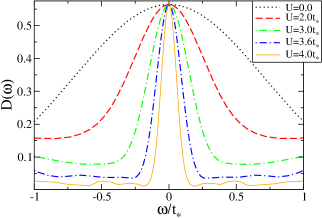
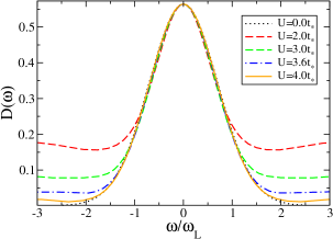
Figure 1: (Color online) Spectral functions for various $U$ showing quasiparticle resonances at Fermi level (left). A simple $x$-axis re-scaling by $Zt_{*}$ leads to a collapse of all of these onto the non-interacting spectral function in the neighbourhood of the Fermi level thus signifying adiabatic continuity and FL behavior.

Since our implementation is new, we would like to benchmark it by comparing our results with other implementations. We begin with the local density of states (DoS) as given by $D(\omega)=-{\rm Im}G(\omega)/\pi$. In Fig. 1 we show the $D(\omega)$ computed at temperature $T=0$ for various $U$ in the metallic regime. The left panel shows the spectral function on ‘non-universal’ scales, i.e. vs. $\omega/t_{*}$, where the Hubbard bands are seen to form with increasing $U$, while the Abrikosov-Suhl resonance at the Fermi level gets narrower. The zero frequency value of the spectral function is also seen to be pinned at the non-interacting ($U=0$) value. Such behavior finds a natural explanation in Fermi liquid (FL) behavior. A simple linear expansion of the self-energy as $\Sigma(\omega)=\Sigma(0)+\left(1-\frac{1}{Z}\right)\omega+{\cal{O}}(\omega^{2})$ when used in Eq. (4) gives $G(\omega)=G_{U=0}(\omega/\omega_{L})$ where $\omega_{L}=Zt_{*}$ is the low energy Fermi liquid scale. Since the quasiparticle weight $Z$ decreases with increasing $U$, thus signifying an increase in effective mass ($m_{*}=m/Z$), the fequency width at half maximum (FWHM) for a hypercubic lattice that is given by $\Delta=2\omega_{L}\sqrt{\ln(2)}$ would decrease with increasing $U$. Another inference from such low frequency scaling behavior is the universality of the low frequency part of the spectral function. On the right panel of Fig. 1, the same spectra as the left panel are plotted as a function of $\omega/\omega_{L}$, and they are all seen to collapse onto the non-interacting limit spectra in the neighbourhood of the Fermi level. All of the above behavior is of course well known and well understood. We nevertheless emphasize that the extent of the FL regime is very small in strong coupling, because as the right panel shows, the scaling collapse is valid for $\omega\lesssim\omega_{L}$, where $\omega_{L}$ is expected to decrease exponentially with increasing $U$. The approximation of IPT does not capture such exponential decrease of $\omega_{L}$, instead predicting an algebraic decrease. Nevertheless, the qualitative behavior from IPT indeed corroborates with other methods such as QMC. IPT has been shown to capture the first order Mott metal-insulator transition qualitatively and in reasonable agreement with other techniques such as NRG [24]. In the $T-U$ plane, the metallic and insulating solutions are known to coexist in a certain region bounded by spinodal lines. The $T=0$ bounds are denoted by $U_{c1}$ and $U_{c2}$. This first order coexistence region may be simply found by computing the temperature or $U$ dependence of the Fermi level density of states ($D(0)=-{\rm Im}G(0)/\pi$) for various values of $U/t_{*}$ or $T/t_{*}$. The resulting phase diagram is shown below in Fig. 2. It agrees well with those reported previously [21, 28].

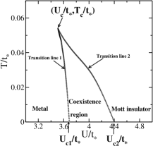
Figure 2: The $U-T$ ‘phase-diagram’ as calculated within IPT is shown here. The solid lines mark the spinodals of the coexistence region where the metallic and the insulating solutions coexist.

The metallic region is a strongly renormalized FL, and thus the properties close to the Fermi level must be governed by a single low energy scale $\omega_{L}$. For universality to hold in the strong coupling region, the spectral function must have the following form:

$$D(\omega;T)=f\left(\frac{T}{\omega_{L}};\frac{\omega}{\omega_{L}}\right)$$ (17)

i.e. it must be a function purely of $\tilde{T}=T/\omega_{L}$ and $\tilde{\omega}=\omega/\omega_{L}$ [31]. In Fig. 3, we show the spectra in strong coupling for fixed $\tilde{T}=0.2$ and increasing $U/t_{*}$. We see that a scaling collapse does not occur implying that the above universal form does not describe the finite temperature IPT results. This non-universal behavior is an artefact of the specific iterated perturbation theory ansatz for the self-energy which is known to yield a non-universal form for its imaginary part [42], namely ${\rm Im}\Sigma_{\rm IPT}(\omega=0)\propto U^{2}T^{2}/t_{*}^{3}$.

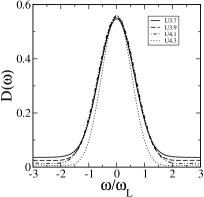
Figure 3: Temperature scaling violated. as a function of temperature for $U/t_{\ast}=2.6$ (dotted), 2.8 (dashed), 3.0 (dotted and dashed), 3.2 (doubly dotted and singly dashed), 3.4 (full line).

The dc resistivity is computed using (7). Again, the pathologies in the imaginary part of the self-energy are reflected in the low temperature FL region in the following way. Although the resistivity does have a $T^{2}$ form, the expected universal scaling form of $(T/\omega_{L})^{2}$ is not obtained [42]. However, surprisingly, the ‘coherence peak’ position, which represents a crossover between low temperature coherent behavior to high temperature incoherent behavior does seem to be a universal feature in strong coupling as seen in Fig. 4 occurring at $\tilde{T}=0.6$. The crosses represent the peak position, and as is seen in the right panel, these crosses line up at a single $\tilde{T}$. Thus the position of the coherence peak may be used to infer the low energy scale in a real material.

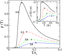
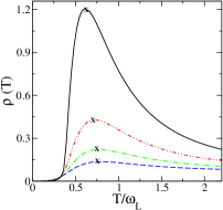
Figure 4: (Color online) Left panel: Theoretically computed resistivity as a function of temperature for various $U/t_{\ast}$ values (indicated as numbers). The crosses indicate the position of the coherence peak. Left panel inset: Experimentally measured [43, 44] resistivity for NiS_2-xSe_x as a function of pressure (indicated as numbers). Right panel: The same resistivities as in the left panel with the temperature rescaled by the low energy coherence scale $\omega_{L}=Zt_{*}$ showing that the coherence peak is indeed a universal feature of the strongly correlated metallic regime.

In the inset of the left panel, we show the experimentally measured [43, 44] resistivity of NiS_2-xSe_x as a function of pressure in Kbar (indicated as numbers). The resistivity for the lowest pressure rises dramatically with increasing $T$, before reaching a coherence maximum, and then decreasing slowly for higher temperatures. With increasing pressures, the initial rise becomes more gradual, and the coherence peak shifts to higher temperatures. An increase in pressure leads to a decrease in lattice spacing, thus increasing $t_{*}$, the hopping parameter, while the local Coulomb repulsion $U$ remains unaffected. Thus increasing pressure can be interpreted as a decrease in the $U/t_{*}$ ratio. A comparison of the inset with the main figure of the left panel clearly indicates qualitative agreement. The initial rise of $\rho(T)$ with $T$ is much sharper in experiment than in theory, but the rest of the features, including a shift of the coherence peak to higher temperatures with increasing pressure, are indeed observed. We emphasize here that the agreement is only qualitative and as such, no attempt is made to obtain quantitative agreement.

We now study the resistivity hysteresis as obtained within IPT approximation.

3.2 Thermal hysteresis

Fig. 5 shows the thermal hysteresis in resistivity obtained through heating and cooling cycles for fixed $U$’s ($t_{\ast}=1$) in the coexistence region. The area enclosed by the hysteresis loop decreases as $U\rightarrow U_{c}$. A full cycle hysteresis is observed only in the region $U_{c}(\sim 3.5)<U<U_{c1}(\sim 3.7)$. For $U<U_{c}$, the metal-insulator transition is continuous and hence of second order while for $U>U_{c1}$ the transition is discontinuous but hysteresis is not obtained.

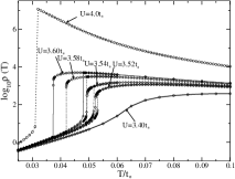
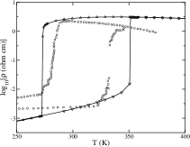
Figure 5: Left panel: The resistivity on a log-scale exhibits thermal hysteresis as a function of temperature when $U_{c}<U<U_{c1}$ (see text for discussion). For $U=3.4t_{*}$ second order transition is observed without hysteresis. For $U=4.0t_{*}$ hysteresis is not observed though the metal-insulator transition is of first order. Right panel: Comparison of theoretically obtained thermal hysteresis ($U=3.6t_{*}$) with experimental observations in V₂O₃ [45].

The hysteresis can be qualitatively explained through the coexistence region in Fig. 2. For $U_{c}<U<U_{c1}$ the $T=0$ ground state is a FL. As one increases $T$ for a fixed $U$, and crosses the spinodal on the right (transition line 2), a first order transition to a paramagnetic insulating state occurs, which upon cooling does not transit to the paramagnetic insulating state until the left spinodal is crossed (transition line 1). Thus as one crosses the coexistence region and reenters via heating/cooling, thermal hysteresis would be obtained. The hysteretic behavior seen in the present theory is naturally very far removed from the rich experimentally observed hysteresis seen e.g. in V₂O₃. The coexistence of metallic and insulating islands has been experimentally observed in thin films [46], as well as in manganites [47], while within DMFT, where spatial inhomogeneities are completely ignored, the coexistence is just that of the metallic and insulating solutions. Experimentally, the resistivity does not increase monotonically with heating or cooling. Instead, multiple steps or avalanches are observed to accompany the hysteretic behavior. While such details are absent in the present theory, nevertheless, we carry out a direct comparison of our hysteresis result with the one found experimentally in doped V₂O₃[45] (right panel of Fig. 5). The purpose of such a comparison being to assess if the half-filled Hubbard model can capture at least the qualitative aspects of real materials. If it does, then the hope would be that a realistic theory based on finite dimensions including spatial inhomogeneities would be able to capture the experimentally observed behavior quantitatively. The best fit of the hysteresis result for a specific interaction ($U=3.6t_{\ast}$), yields $t_{*}\sim 7305\mathrm{K}$ $(0.63\mathrm{eV})$. This agrees well with independent bandstructure calculations for V₂O₃ [48] and is of the right magnitude.

We now focus on optical transport in the next subsection.

3.3 Optical conductivity:

As can be naturally expected, changes in interaction strength $U/t_{*}$ and especially the Mott MIT affect dynamical or optical transport properties strongly. Fig. 6 shows the computed $T=0$ optical conductivity $\sigma(\omega)$ as $U/t_{*}$ increases from a low value of 1.0 to a moderately strong value of 3.0. The inset shows the corresponding spectral functions. Several very interesting features can be seen.

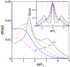
Figure 6: (Color online) The main panel shows the zero temperature optical conductivity for $U/t_{*}$ values ranging from 1.0 to 3.0 (indicated by numbers). The inset shows the corresponding spectral functions.

As $U$ increases, a strong absorption feature emerges at $\sim U/2$ for $U\gtrsim 2t_{*}$, while a second peak at $\sim U$ emerges beyond 3$t_{*}$. For low values, none of these features may be distinguished. The first peak arises because of excitations between either of the Hubbard bands and the Fermi level, while the second peak represents excitations between the lower and upper Hubbard band. The zero frequency Drude peak is also present, but is not visible, since it has a Dirac-delta function form. The changes in optical conductivity are naturally understood through the inset of Fig. 6. For low values of $U/t_{*}$, a single featureless spectral function is obtained, while the emergence of distinct Hubbard bands in the spectra mark the emergence of the first and second absorption peaks in the optical conductivity. At around the half bandwidth ($\omega\simeq 1.15t_{*}$) a universal crossing point is is seen in the spectra.

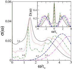
Figure 7: (Color online) The main panel shows the zero temperature optical conductivity for $U/t_{*}$ values ranging from 3.0 to 5.0 (indicated by numbers). The inset shows the corresponding spectral functions.

The effect of Mott transition on the optical absorption is illustrated clearly in Fig. 7, which is similar to the previous figure, except that the values of $U/t_{*}$ considered here increase from 3.0 to 5.0. The transition from the correlated metallic phase to the Mott insulator phase occurs at $U/t_{*}\simeq 4.5$, where, within IPT, a large gap $\sim U-2t_{*}$ is known to form. The main panel shows optical conductivity as a function of $\omega/t_{*}$. In the metallic phase ($U<U_{c2}$), the first absorption peak is seen to get narrower and surprisingly gets red-shifted as the Mott transition is approached. The second absorption peak begins to dominate as $U\rightarrow U_{c2}$ and becomes the sole feature in the Mott insulating phase. The $U>U_{c2}$ optical conductivity is seen to possess a clear optical gap, which increases with increasing $U$ and reflects the presence of the gap in the density of states (see inset).

The temperature evolution of the optical conductivities is equally interesting. In Fig. 8 we show the $\sigma(\omega;T)$ behavior for various $T$’s for a moderately strong interaction strength of $U=3.0t_{*}$. The inset again shows the corresponding spectral functions.

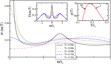
Figure 8: (Color online) The main panel shows the temperature evolution of optical conductivity for $U/t_{*}=3.0$. The left inset shows the corresponding spectral functions and the right inset shows the resistivity at $T=0.2t_{\ast}$. M marks for metallic ($d\rho/dT>0$) and I marks for insulating ($d\rho/dT<0$) behavior.

The first absorption peak at lower temperatures loses spectral weight as temperature increases, which is gained by the second peak, and again an almost universal crossing point is seen, marking the frequency across which the transfer of spectral weight occurs. The Drude peak at $\omega=0$ diminishes in height, consistent with the dc conductivity values, and disappears completely at $T=0.2$ by forming a shoulder-like feature at higher frequency $\omega\sim 2.5t_{\ast}$.

An earlier investigation[49] (though it was not exactly calculated for the half-filled HM) claimed that the shoulder formation is actually shifting of Drude peak (pseudo-Drude peak) and the phase is metallic. However, here we argue that this arises due to the pseudogap formation in the DoS (see the left inset) and it is actually an insulating state since $d\rho(T)/dT<0$ (see the right inset) and the phase lies in the crossover regime.

The universal crossing point, known as the isosbestic point in the metallic phase has been observed in several materials, e.g. V₂O₃ [50], NiS_2-xSe_x [51], La_2-xSr_xCuO₄ [52], La_1-xSr_xTiO₃ [53]. Occurrence of isosbestic points are not well-explained. Nevertheless such a point is believed to have a close connection with $f$-sum rules and its location is associated to microscopic energy scales in correlated systems [54, 55]. Here, we see that the dynamics also exhibit a similar feature indicating an even more general basis for its existence. If we use our earlier estimation of $t_{\ast}$ (0.6 eV) for V₂O₃ or the LDA-calculated value, we find that the isosbestic point arises at $\sim$ 0.9-1.0 eV which lies in the mid-infrared range, and which is close to that seen in a recent infra-red spectroscopy measurement [50] i.e. at 6000 cm^-1 ($\sim 0.7$ eV).

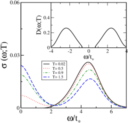
Figure 9: (Color online) The main panel shows optical conductivity for temperatures $T/t_{*}=0.02,0.5,0.9$ and $1.5$. The inset shows the corresponding spectral function which exhibits negligible changes as temperature is increased.

Finally we show the optical conductivity for the Mott insulating regime ($U/t_{*}=4.7$) evolving with temperature in Fig. 9. A single absorption peak is seen at low temperatures, and as $T$ increases, spectral weight is transferred from this peak to lower frequencies, and the absorption peak diminishes, and experiences a blue shift. The spectral function exhibits negligible change as a function of temperature and although, there is indeed, an exponentially small rise in the density of states in the neighbourhood of the Fermi level, it visually appears to coincide with the $T=0$ DoS.

4 Conclusion

A systematic study of the half-filled Hubbard model within dynamical mean field theory is carried out, with the focus being on universality, scaling and qualitative comparison to experiments. We reformulate a well-known and extensively employed impurity solver for the effective impurity problem that the lattice problem gets mapped onto within DMFT, namely the iterated perturbation theory, such that some of the problems with previous implementations have been overcome. We find that the coherence peak in the resistivity is a universal feature. A comparison with experimental measurements of resistivity in Se doped NiS₂ with varying pressure yields qualitatively excellent agreement. Thermal and pressure driven hysteresis is shown to be qualitatively explicable within this scenario, and again, a comparison of thermal hysteresis with experiments in V₂O₃ are seen to yield a reasonable number for the hopping integral. The transfer of spectral weight across the Mott transition and the isosbestic points have been highlighted in the study of optical conductivity. We conclude that the Hubbard model does indeed represent an appropriate phenomenological model that can qualitatively explain a large range of phenomena observed in transition metal oxides. This offers hope for more detailed material specific studies such as those employing LDA+DMFT [56, 57, 58] approaches to obtain quantitative agreement with experiments.

Appendix A: Analytical calculation of $U_{c1}$ and $U_{c2}$ at $T=0$

In this section, we demonstrate that a pole structure ansatz for the Green’s functions and self energy combined with the IPT equations yields $U_{c1}$ and $U_{c2}$, the bounds of the $U$ interval where the metallic and insulating solutions coexist at zero temperature.

If $\mathcal{G}$ has simple poles at $\pm\omega_{0}$ with equal residue $\alpha/2$ (due to symmetry), then the singular part of $\mathcal{G}$ may be expressed as

$$\mathcal{G}(\omega)=\frac{\alpha}{2}\bigg{[}\frac{1}{\omega-\omega_{0}}+\frac{1}{\omega+\omega_{0}}\bigg{]}=\alpha\frac{\omega}{\omega^{2}-\omega^{2}_{0}}$$ (18)

Now using the Dyson equation (Eq. (5)) and the moment expansion of the Hilbert transform, we get

$$\Sigma(\omega)=\frac{1}{\alpha}\frac{\omega^{2}-\omega^{2}_{0}}{\omega}-\omega+\Sigma(\omega)-\frac{M_{2}}{\omega-\Sigma(\omega)}$$

Thus

$$\Sigma(\omega)=\omega-\frac{M_{2}}{\frac{1}{\alpha}\frac{\omega^{2}-\omega^{2}_{0}}{\omega}-\omega}$$ (19)

Therefore poles occur at

$$\omega^{\prime}_{0}=\pm\frac{\omega_{0}}{\sqrt{1-\alpha}}$$ (20)

Using the structure of $\mathcal{G}$ in the IPT equations, it is easy to see that poles at $\pm\omega_{0}$ in $\mathcal{G}$ will give rise to poles in the self energy at $\pm\omega_{0}$ and $\pm 3\omega_{0}$. Only the latter are physically acceptable, since the former leads to a self-consistent value of the residue $\alpha$ equal to $0$. So when $\omega^{\prime}_{0}=\pm 3\omega_{0}$, $\alpha$ turns out to be 8/9.

The singular part and the FL part of the self energy may be expressed in a combined way as

$$\Sigma(\omega)=\frac{U^{2}\alpha^{3}}{8}\bigg{[}\frac{1}{\omega-3\omega_{0}}+\frac{1}{\omega+3\omega_{0}}\bigg{]}-\left(1-\frac{1}{Z}\right)\omega$$ (21)

This gives

$$\Sigma(\omega_{0})=-\frac{U^{2}\alpha^{3}}{32\omega_{0}}-\left(1-\frac{1}{Z}\right)\omega_{0}$$ (22)

Now $\mathcal{G}^{-1}(\omega_{0})=0$. So the Dyson equation (Eq. (5)) gives

$$\Sigma(\omega_{0})=-G^{-1}(\omega_{0})=-\gamma(\omega_{0})-\frac{M_{2}}{\gamma(\omega_{0})}=-\omega_{0}+\Sigma(\omega_{0})-\frac{M_{2}}{\omega_{0}-\Sigma(\omega_{0})}$$ (23)

and hence, after rearranging we get

$$\omega^{2}_{0}=Z\left(M_{2}-\frac{U^{2}\alpha^{3}}{32}\right)$$ (24)

The above result shows that the pole position is proportional to the square root of the quasiparticle weight. The transition from the metallic to the insulating regime occurs when $\omega_{0}=0$.This occurs when $M_{2}=\frac{U^{2}\alpha^{3}}{32}$, i.e. for HCL, with $\alpha=8/9$,

$$\frac{U_{c2}}{t_{\ast}}=\frac{4}{\alpha^{3/2}}=\frac{27}{4\sqrt{2}}$$ (25)

To get $U_{c1}$, we refer back to Eq. (13) which holds in the insulating phase. This self consistent equation for the pole residue in the insulating phase $\alpha$ has real roots only when $U^{2}\geq 27M_{2}$, i.e. for HCL

$$U_{c1}=\frac{3\sqrt{3}}{\sqrt{2}}t_{\ast}$$ (26)

The above analysis shows that we can analytically estimate $U_{c1}$ and $U_{c2}$ within the same framework.

References

- [1] J. C. Hubbard, Proc. R. Soc. A 276, 238 (1963).
- [2] M. C. Gutzwiller, Phys. Rev. Lett. 10, 59 (1963).
- [3] J. Kanamori, Prog. Theor. Phys. 30, 275 (1963).
- [4] M. C. Gutzwiller, Phys. Rev. Lett. 10, 159 (1963).
- [5] M. Greiner et al., Nature 415, 39 (2002).
- [6] N. F. Mott, Metal Insulator Transitions (Taylor and Francis, Bristol, 1990).
- [7] M. Imada et al., Rev. Mod. Phys. 70, 1039 (1998).
- [8] P. A. Lee, N. Nagaosa, and X.-G. Wen, Rev. Mod. Phys. 78, 17 (2006).
- [9] M. Jarrell, Phys. Rev. Lett. 69, 168 (1992).
- [10] K. Wakabayashi and K. Harigaya, J. Phys. Soc. Japan 72, 998 (2003).
- [11] J. Fernández-Rossier, Phys. Rev. Lett. 99, 177204 (2007).
- [12] D. R. Penn, Phys. Rev. Lett. 142, 350 (1966).
- [13] D. Poilblanc and T. M. Rice, Phys. Rev. B 39, 9749 (1989).
- [14] A. R. Bishop, Europhys. Lett. 14, 157 (1991).
- [15] J. C. Hubbard, Proc. R. Soc. A 277, 237 (1963).
- [16] J. C. Hubbard, Proc. R. Soc. A 281, 401 (1964).
- [17] M. C. Gutzwiller, Phys. Rev. 134, A923 (1964).
- [18] G. Kotliar and A. E. Ruckenstein, Phys. Rev. Lett. 57, 1362 (1986).
- [19] E. H. Lieb and F. Y. Wu, Phys. Rev. Lett. 20, 1445 (1968).
- [20] W. Metznerand and D. Vollhardt, Phys. Rev. Lett. 62, 324 (1989).
- [21] A. Georges, G. Kotliar, W. Krauth, and M. J. Rozenberg, Rev. Mod. Phys. 68, 13 (1996).
- [22] T. Maier, M. Jarrell, T. Pruschke, and J. Keller, Eur. Phys. J. B 13, 613 (2000).
- [23] A. Georges and W. Krauth, Phys. Rev. Lett. 69, 1240 (1992).
- [24] R. Bulla, T. A. Costi, and D. Vollhardt, Phys. Rev. B 64, 04103 (2001).
- [25] M. Caffarel and W. Krauth, Phys. Rev. Lett. 72, 1545 (1994).
- [26] K. Yosida and K. Yamada, Prog. Theor. Phys. 46, 244 (1970).
- [27] A. Georges and W. Krauth, Phys. Rev. B 48, 7167 (1993).
- [28] M. J. Rozenberg, G. Kotliar, and X. Y. Zhang, Phys. Rev. B 49, 10181 (1994).
- [29] D. E. Logan, M. P. Eastwood, and M. A. Tusch, J. Phys.: Condens. Matter 10, 2673 (1998).
- [30] N. S. Vidhyadhiraja and D. E. Logan, Eur. Phys. J. B 39, 313 (2004).
- [31] A. C. Hewson, The Kondo Problem to Heavy Fermions (Cambridge University Press, Cambridge, 1993).
- [32] W. H. Press et al., Numerical Recipes in Fortran 77 (Cambridge University Press, Cambridge, 1992).
- [33] M. B. Fathi and S. A. Jafari, Physica B 405, 1658 (2010).
- [34] A. Khurana, Phys. Rev. Lett. 64, 1990 (1990).
- [35] G. D. Mahan, Many-particle physics (Plenum Press, New York, 1990).
- [36] N. S. Vidhyadhiraja et al., Europhys. Lett. 49, 459 (2000).
- [37] N. S. Vidhyadhiraja, Europhys. Lett. 77, 36001 (2007).
- [38] T. Saso, J. Phys. Soc. Japan 66, 1175 (1997).
- [39] M. J. Rozenberg, G. Kotliar, and H. Kajueter, Phys. Rev. B 54, 8452 (1996).
- [40] F. Gebhard, The Mott Metal-Insulator Transition (Springer, Berlin, 1997).
- [41] W. Anglin and J. Lambek, The Heritage of Thales (Springer-Verlag, New York, 1995), p. p 133.
- [42] S. F. A. Georges and T. A. Costi, J. Phys. IV France 114, p 165 (2004).
- [43] J. M. Honig and J. Spalek, Chem. Mater. 10, 2910 (1998).
- [44] N. Mori et al., Solid State Physics under Pressure: Recent Adv. Anvil Devices p 247 (1985).
- [45] H. Kuwamoto, J. M. Honig, and J. Appel, Phys. Rev. B 22, 2626 (1980).
- [46] C. Grygiel et al., J. Phys.: Condens. Matter 20, 472205 (2008).
- [47] D. D. Sarma et al., Phys. Rev. Lett. 93, 097202 (2004).
- [48] L. H. Mattheiss, J. Phys.: Condens. Matter 6, 6477 (1994).
- [49] T. Mutou and H. Kontani, Phys. Rev. B 74, 115107 (2006).
- [50] L. Baldassarre et al., Phys. Rev. B 77, 113107 (2008).
- [51] A. Perucchi et al., Phys. Rev. B 80, 073101 (2009).
- [52] S. Uchida et al., Phys. Rev. B 43, 7942 (1991).
- [53] T. Katsufuji et al., Phys. Rev. Lett. 75, 3497 (1995).
- [54] M. Eckstein, M. Kollar, and D. Vollhardt, Journal of Low Temperature Physics 147, 279 (2007).
- [55] J. K. Freerick and T. P. Devereaux, Physica B 378–380, 650 (2006).
- [56] K. Held et al., Phys. Rev. Lett. 86, 5345 (2001).
- [57] D. Vollhardt et al., J. Phys. Soc. Japan 74, 136 (2005).
- [58] G. Kotliar et al., Rev. Mod. Phys. 78, 865 (2006).