Spin and Charge Fluctuations in the $\alpha$-structure Layered Nitride Superconductors

Abstract

To explore conditions underlying the superconductivity in electron-doped TiNCl where T_c = 16 K, we calculate the electronic structure, Wannier functions and spin and charge susceptibilities using first-principles density functional theory. TiNCl is the first high-temperature superconductor discovered in the $\alpha$-structure of the layered transition-metal nitride family MNCl (M=Ti, Zr, Hf). We construct a tight-binding model based on Wannier functions derived from the band structure, and consider explicit electronic interactions in a multi-band Hubbard Hamiltonian, where the interactions are treated with the random phase approximation (RPA) to calculate spin and charge susceptibility. The results show that, consistent with TiNCl being a nonmagnetic material, spin fluctuations do not dominate over charge fluctuations and both may have comparable impact on the properties of the doped system.

I Introduction and Background

High-temperature superconductivity has been a widely pursued subject for condensed matter physicists for over two decades. There are several classes of materials where unconventional superconductivity is found: cuprates whose highest T_c’s remain unrivaled, the recently discovered and intensively studied iron pnictides, Na_1-xCoO₂ intercalated with H₂O, BaBiO₃ doped by K, the Pu-based “115” heavy fermion series, and the transition metal nitride halide MNX (M=Zr, Hf; X=Cl, Br, I). MNX crystallizes in two structures, labeled $\alpha$ and $\beta$. The Zr and Hf members were found to be superconducting with unprecedented critical temperatures for nitrides (15K, 25K) in the $\beta$-structure, which is isostructural to SmSI, and contains double-honeycomb layers of alternating M and N atoms beta-structure . The sister compound TiNCl with $\alpha$-structure has now been discovered to superconduct (16K) as well.TiNCl-SC

Based on many examples now, layered structures seem to favor high-temperature superconductivity. The reduced dimensionality promotes various instabilities associated with Fermi surface nesting. Due to electron-electron interactions, many parent compounds of HTSCs exhibit long-range magnetic order, such as antiferromagnetism (AFM) in cuprates and iron pnictides. The AFM order needs to be destroyed upon doping, by electrons or by holes, to open the way for superconductivity. This is not the case for non-magnetic MNX, which are band insulators with a band gap of $2-4$ eV, and the transition metal $d$ states make up most of the lower conduction bands HfNCl-band .

Both the $\alpha$- and $\beta$-polymorphs are quasi-2D structures with large interlayer spacing and weak van der Waals coupling between layers. When doped with electrons, A_xMNX (A being alkali metals) remains insulating at low concentration, then suddenly become superconducting at about $x=0.13$ in HfNCl and $x=0.06$ in ZrNCl, and maintain a relatively constant T_c up to $x=0.5$ [LixZrNCl-Tcdoping, ]. The superconducting transition temperature can be as high as $26$ K, discovered in Li_x(THF)_yHfNCl HfNCl-Nature1998 . It has also been found that T_c may be correlated with the interlayer spacing, which can be tuned by intercalation of different sized molecules HfNCl-Tcspacing . Also, the electron doping can be substituted by ion vacancy of the Cl atoms with similar superconductivity being found MNCl1-x-SC . In a theoretical treatment by Bill et al., the dynamical screening of electronic interactions in these materials was modeledplasmon1 ; plasmon2 by conducting sheets spaced by dielectrics.Jain1985 A fully open large superconducting gap without nodes was observed with tunneling spectroscopy. LiZrNCl-SCgap ; LiTHFHfNCl-gap1 ; LiTHFHfNCl-gap2

Experimental observations from several perspectives confirm that MNX are not electron-phonon BCS superconductors: (1) measured isotope effects are small;HfNCl-isotope ; LixZrNCl-isotope (2) specific heat measurementsLixZrNCl-spheat indicate a small mass enhancement factor; (3) the density of states at the Fermi level is small (when electron doped), and T_c is almost independent of the doping level in the range $0.15<x<0.5$. As a feature peculiar to this system, T_c actually increases as the metal-insulator transition at $x_{cr}$=0.06 is approached, rather than following the common dome shape with doping. Linear response calculations also agree on the small electron-phonon coupling constant LixZrNCl-phonon that cannot account for the observed T_c. The impressive high transition temperatures and easy tunability of carrier concentrations (and sometimes effective dimensionality) suggest there is potential to reach higher T_c in this class.Yamanaka-review

The possible candidates of pairing mechanism responsible for the observed high T_c are spin and charge fluctuations, which have been discussed by both experimentalists and theorists, but opinions remain controversial. The specific heat measurement on Li_xZrNCl is suggestive of relatively strong coupling superconductivity, based on the observed large gap ratio and specific jumpLixZrNCl-spheat at T_c. The inter-layer spacing dependence of T_c reveals the close relation between the pairing interaction and topology of the Fermi surface HfNCl-Tcspacing , implying a spin and/or charge induced superconductivity. The magnetic susceptibility measurement of heavily doped Li_x(THF)_yHfNCl indicates low carrier density and negligible mass enhancement factor, in favor of charge fluctuations over the spin fluctuations.Li(THF)HfNCl-X-expt

A detailed measurement of the doping dependence of specific heat and magnetic susceptibility has been performed on Li_xZrNCl and the data were compared with calculations based on a model Hamiltonian LixZrNCl-Xs-expt ; Kuroki-FLEX , which shows correlation between T_c and magnetic susceptibility. Some change is occurring that affects both, but a causal relationship has not been established. There have been several band structure calculations for ZrNCl and HfNCl that provide the basis for more specific studies, mostly in the superconducting $\beta$-structure.HfNCl-band ; ZrHfNCl-band1 ; ZrHfNCl-band2 ; ZrNCl-band

Recently, Yamanaka et al TiNCl-SC reported superconductivity in the alkali metal intercalated $\alpha$-TiNCl, with T_c up to $16.5$ K. This is the first MNX compound found to be superconducting in the $\alpha$-structure. The lack of Fermi surface nesting in $\alpha$-Li_xTiNCl seems to exclude large magnetic fluctuations, and its low carrier density character is indicative of charge fluctuations as a more likely driving force. Theoretically, charge fluctuation induced superconductivity has been discussed in the Hubbard model ChargeFluc1 ; ChargeFluc2 , the $d$-$p$ model ChargeFluc3 , and been applied to study Na_xCoO${}_{2}\cdot y$H₂O NaCoO2-FLEX ; NaCoO2-RPA and organic molecular superconductors ChargeFluc-organicSC . A more detailed investigation of the electronic structure and dynamical spin/charge susceptibility is needed to study the superconducting mechanism in $\alpha$-TiNCl. In the present work, we conduct a theoretical calculation of spin and charge susceptibilities using a many-body Hamiltonian, based on a realistic band structure calculated by density functional theory.

II Crystal Structure

The $\alpha$-structureTiNCl-SC of the MNX class of compounds, often called the FeOCl structure, is shown in Fig. 1, with structural data given in Table 1. The $\alpha$-structure TiNCl belongs to space group Pmmn (#59), with 6 atoms per unit cell occupying the following sites: Ti($2b$) (0,$\frac{1}{2},z_{Ti}$), N($2a$) ($\frac{1}{2},\frac{1}{2},z_{N})$ and Cl($2a$) (0,0,$z_{Cl}$). The generators of Pmmn are two simple reflections $x\rightarrow-x$ and $y\rightarrow-y$, and the non-symmorphic reflection $z\rightarrow-z$ followed by a ($\frac{1}{2},\frac{1}{2},0)$ translation.

The Ti-N net within TiNCl is topologically equivalent to that of a single NaCl layer. There is strong buckling this Ti-N net perpendicular to the $b$ direction, such that neighboring chains which are directed along $a$ differ in height. These chains are themselves somewhat buckled, all of this leading to the placement of Ti ions $\pm$0.8 Å from the average height, and N ions $\pm$0.4 Å from the average height. The Ti ions are two-fold coordinated by Cl ions lying in the $y-z$ plane; the breaking of square symmetry of the TiN layer by its strong buckling, can be regarded as “due to” this positioning of the Cl ions.

Finally, each Ti is six-fold coordinated by four N and two Cl atoms. The two Ti-N bonds have very close lengths of $2.008$ Å and $2.015$ Å, respectively, though the N ions lie at different heights in the $x$ and $y$ directions. Very roughly, the Ti ion is in octahedral coordination (see Fig. 5 of Ref. [TiNCl-SC, ]), with approximate axes (1,0,0) (toward two neighboring N ions), and (0,1,1) and (0,1,-1) (each toward one N and one Cl ion), and indeed a rough $t_{2g}-e_{g}$ splitting of the Ti $3d$ states results. The Ti-Ti distance is $3.003$ Å, not much larger than that of Ti-N due to the buckled layer structure, so in the tight-binding model we construct in the next section, the hoppings between Ti sites are also important.

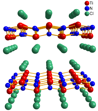
Figure 1: Crystal structure of $\alpha$ phase TiNCl (Pmmn, #59). Viewpoint is along the b-axis, perpendicular to the buckling of the Ti-N net. The buckled Ti-N layer leaves each Ti coordinated (roughly octahedrally) by 4 N and 2 Cl atoms. The Cl coordinates with Ti along the b-axis, which accounts for its orthorhombic structure.

The experimental lattice constants and atomic positions, and relaxed structure parameters with respect to total energy, which are used in our calculation, are listed in Table 1. The calculations (see below) confirm the expected formal valences. The calculated lattice constants are 1-1.5% smaller than the experimental values, but this has little effect on the electronic structure. TiNCl is still calculated to be an ionic insulator and its theoretical gap is similar to what is calculated using the experimental lattice parameters.

	$a$	$b$	$c$	$z_{Ti}$	$z_{N}$	$z_{Cl}$
Expt.	$3.938$	$3.258$	$7.800$	$0.1011$	$0.0509$	$0.3322$
Theory	$3.891$	$3.200$	$7.699$	$0.1011$	$0.0522$	$0.3384$

Table 1: Lattice constants (in units of Å) and internal structural parameter $z$ for the three atoms. Experimental values are from Ref. TiNCl-SC, . The theoretical values are our optimized values.

III Band Structure and Wannier Functions

III.1 Methods

The band structure has been computed by the full-potential local orbital minimal basis set method implemented in the FPLO code.FPLO The exchange correlation is treated by the generalized gradient approximation GGA96,GGA96 and the k-mesh used is $16\times 16\times 8$. The effect of spin-orbit coupling is small so calculations were done in the scalar relativistic scheme.

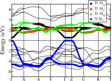
Figure 2: (color online) Band structure of TiNCl along the orthorhombic symmetry lines, calculated with the GGA exchange-correlation functional. The thick “fatbands” are the tight-binding representation determined by the Wannier functions labeled in the inset, chosen to represent accurately the bands at and around the Fermi level after doping.

III.2 Electronic Structure

The calculated band structure of pristine TiNCl is shown in Fig. 2 and is generally consistent with that presented by Yamanaka et al.TiNCl-SC plotted along other lines in the zone. It is an insulator with a calculated energy gap of $0.5$ eV. The real band gap may be as large as $1$ eV, based on the common observation that LDA and GGA underestimates gaps in insulators. The band structure exhibits clearly a two-dimensional feature, gauged from the general flatness of bands along the $\Gamma-Z$ direction perpendicular to the layers. The states on either side of the gap are very two-dimensional, considering the extreme flatness of those bands along $\Gamma$-Z.

The twelve valence bands are made of six N $2p$ and six Cl $3p$ states, and the conduction band is comprised of ten Ti $3d$ states. The $3d$ bands show a “$t_{2g}-e_{g}$” crystal field splitting (three states below and two above), that arises in spite of the nonequivalence of the five $3d$ orbitals in this structure. As can be seen in the partial density of states plotted in Fig. 3, there is $3d$ weight in the valence bands and N weight in the conduction bands, reflecting substantial N $2p$ - Ti $3d$ hybridization in addition to the ionic character reflected in their formal charges.

Whereas the $3d$ environment appears locally to be pseudo-cubic, the low site symmetry severely splits the N $2p$ states, with $2p_{x}$ and $2p_{y}$ becoming quite distinct. The top valence band is primarily N $2p_{x}$ character, which extends down to $-5$ eV. The N $p_{y}$ and $p_{z}$ bands have their maximum 1 eV lower, and the Cl $2p$ weight is concentrated at the bottom of the valence bands.

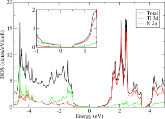
Figure 3: (color online) Total and partial density of states of TiNCl, showing the Ti $3d$ - N $2p$ mixing. The inset figure is a blown-up of the region near Fermi level.

The inset in Fig. 3 shows an enlargement of the total and atom-projected DOS around the Fermi energy. The onset at 0.5 eV and the smooth slope to 1.2 eV is characteristic of a two-dimensional band which becomes non-parabolic away from the band edge, and strongly so in the 1.2-1.5 eV region. At 1.5 eV the onset of the second band, with its much heavier mass, is clear. However, the DOS does not have the sharp step at the top of the valence band that is characteristic of a 2D system.

The Ti $3d$ orbitals are lifted in degeneracy entirely by the orthorhombic point group site symmetry, but as mentioned above the conduction bands are separated by a crystal field analogous to cubic $t_{2g}-e_{g}$ splitting. Checking the band character reveals that, in terms of $3d$ orbitals expressed in terms of the orthorhombic coordinate axes, $d_{xy},d_{z^{2}},d_{xz}$ have most of the weight in the $0.5-3$ eV region, and $d_{yz},d_{x^{2}-y^{2}}$ are in a higher energy window of $4-6$ eV. Thus it is feasible, in a low-energy tight-binding model, to include only Ti $d_{xy},d_{z^{2}},d_{xz}$ and N $2p_{x}$ states. Plotted on top of the DFT bands in Fig. 2 is the tight-binding fit using the Wannier functions. The representation of the full $t_{2g}$ complex is excellent, as is that of the top of the upper valence band.

The distance between TiNCl slabs and the weak inter-layer coupling allows intercalation of alkali atoms, which act as electron donors. This feature validates the rigid band shift approximation in simulating doping. Doped-in electronic carriers will go into the single lowest conduction band, which is quite two-dimensional as mentioned above but is dispersive within the plane. This band has strong Ti $3d_{xy}$ character, similar to the in-plane $4d$ character in ZrNCl. The Fermi surface of electron-doped TiNCl is an oval centered at the $\Gamma$ point. This point has some relevance for the superconductivity, since with a single Fermi surface there can be no nesting of disconnected Fermi surfaces, such as are proposedKuroki-FLEX to play an important role in many other layered superconductors, such as Fe pnictides, as well as $\beta$-structured ZrNCl and HfNCl. The similar characters of TiNCl and ZrNCl, and their similar values of T_c, suggest that possible nesting of Fermi surfaces is not an important feature for pairing in the materials.

III.3 Wannier Functions

Because the susceptibilities we will calculate have a number of local orbital matrix elements equal to the 4th power of the number of orbitals retained, we have calculated selected low-energy Wannier functions (WFs) that will be used to construct our many-body Hamiltonian, using projections of the Bloch states onto the corresponding atomic orbitals. The four atomic orbitals mentioned above allow us to reproduce the bands on either side of the gap: Ti $d_{xy},d_{z^{2}},d_{xz}$ and N $p_{x}$. While the Ti “$t_{2g}$” orbitals are not optimal in diagonalizing the local “octahedral” symmetry, they and their relation to the $2p_{x}$ orbital are more readily visualized. Since the RPA calculations described below were performed in the electron-doped region where the Fermi level is shifted into the conduction bands, considering only the N $p_{x}$ WF in the valence band is sufficient to understand the $\mathbf{q}$-dependence. Aside from being farther removed in energy, the remainder of the valence bands form a complex of bands spread uniformly over the zone, contributing little to any $\mathbf{q}$-dependence.

The Ti-N layer is strongly buckled and there are 2 Ti and 2 N atoms per unit cell with different $z$ coordinates. the actual tight-binding model contains 8 bands and 8 WFs, but WFs on symmetry related ions are symmetry equivalent. Overall the Wannier orbitals generate a well represented band structure compared to the DFT bands within the energy window of interest, as shown in Fig. 2.

The hopping amplitudes of the Wannier orbitals are listed in Table 2. Hopping integrals smaller than $0.05$ eV were not listed because they only marginally alter the band structure and obfuscate interpretation. The on-site energies of the “$t_{2g}$” orbitals are $2.25\pm 0.08$eV, lying within the largest peak of the DOS. The $p_{x}$ energy is $-3.22$eV, in the middle of the valence bands. Thus there is a $5.5$eV separation of valence and conduction band centers, and a gap of $0.5$eV.

The dispersion within the pair of valence $p_{x}$ bands is represented largely by hopping between neighboring $p_{x}$ WFs (recall, the $p_{x}$ WF contains some $d$ character, and vice versa), both being about $0.5$eV. Hopping amplitudes to the $d$ orbitals are $t_{pd}\approx 0.2-0.3$eV. In the conduction bands, the $d_{xy}$ orbital has hopping amplitude $|t|\sim 0.17$eV to its partner within the cell as well as to its replicas in neighboring cells in both directions. The hopping to the $p_{x}$ orbital (0.33 eV) is twice as large, and apparently is the dominant contributor to the $3.5$eV bandwidth. Due to the relative orientations, hopping to the other $d$ WFs is no more than half as large as the $d_{xy}-d_{xy}$ one. The other two $d$ WFs form rather narrow bands, reflected by smaller hopping amplitudes; note that both have hopping to the $p_{x}$ orbital of $0.21-0.24$eV.

$(\mu,\nu)$	$[0,0,0]$	$[1,0,\Delta z]$	$[0,1,\Delta z]$	$[1,1,\Delta z]$	$[2,0,0]$	$[0,2,0]$
$(d_{xy},d_{xy})$	$2.33$			$-0.16$	$-0.17$	$-0.18$
$(d_{xy},d_{z^{2}})$				$-0.08$
$(d_{xy},d_{xz})$				$0.07$		$-0.11$
$(d_{z^{2}},d_{z^{2}})$	$2.18$			$-0.05$
$(d_{z^{2}},d_{xz})$				$0.19$	$0.07$
$(d_{xz},d_{xz})$	$2.25$				$-0.05$	$0.13$
$(d_{xy},p_{x})$			$-0.33$
$(d_{z^{2}},p_{x})$		$0.24$	$0.22$
$(d_{xz},p_{x})$			$0.21$
$(p_{x},p_{x})$	$-3.22$			$0.51$	$0.47$	$0.14$

Table 2: Nearest, 2nd, and 3rd neighbor hopping integrals in units of eV. The hopping vectors are in units of [a/2, b/2, c], and $\Delta$z represents the difference between the z coordinates of the two orbitals. This representation is purely two-dimension (no coupling along the $c$ axis).

IV Many-body Hamiltonian and Random Phase Approximation

The random phase approximation (RPA) applies an interaction to the non-interacting Hamiltonian

$$H_{0}=\sum_{\mathbf{k},ab}H_{ab}^{\mathbf{k}}c_{\mathbf{k},a}^{\dagger}c_{\mathbf{k},b},$$ (1)

where $a,b$ are composite orbital and spin indices of the basis Wannier orbitals. The interaction Hamiltonian, in general, is the following symmetric form

$$H_{1}=\frac{1}{2}\sum_{i}\sum_{abcd}U_{abcd}c_{ia}^{\dagger}c_{ib}c_{ic}^{\dagger}c_{id}+\sum_{\langle i,j\rangle}\sum_{abcd}V_{abcd}c_{ia}^{\dagger}c_{ib}c_{jc}^{\dagger}c_{jd},$$ (2)

where $U$ and $V$ represent on-site and inter-site (only nearest neighbors) interactions, respectively. (2) can be Fourier transformed into

$$H_{1}=\frac{1}{2N}\sum_{\mathbf{kpq}}\sum_{abcd}F_{abcd}(\mathbf{q})c_{\mathbf{k},a}^{\dagger}c_{\mathbf{k+q},b}c_{\mathbf{p+q,}c}^{\dagger}c_{\mathbf{p}d},$$ (3)

in which $F_{abcd}(\mathbf{q})=U_{abcd}+\gamma(\mathbf{q})V_{abcd}$ is the interaction kernel matrix. In the second term, $\gamma(\mathbf{q})=\sum_{l}e^{i\mathbf{q}\cdot\mathbf{R}_{l}}$ ($l$ running over the nearest neighbor pairs of sites) is the structure factor, which brings in $\mathbf{q}$-dependence into $F_{abcd}(\mathbf{q})$. The bare susceptibility is calculated as

$$\chi_{abcd}^{0}(\mathbf{q},\omega)=\sum_{\mathbf{k}}G_{ad}(\mathbf{k},\omega)G_{cb}(\mathbf{k+q},\omega),$$ (4)

where $G_{ab}(\mathbf{k},\omega)$ is the non-interacting Green’s function

$$G_{ab}(\mathbf{k},\omega)=\sum_{n}\frac{\left\langle a\right|n\mathbf{k}\rangle\langle n\mathbf{k}\left|b\right\rangle}{\omega+\mu-\varepsilon_{n\mathbf{k}}},$$ (5)

and the summation is taken over all bands. Applying RPA, which sums up the higher order diagrams in the geometric series, we have the full susceptibility presented in a matrix equation

$$\chi(\mathbf{q},\omega)=[I+\chi^{0}(\mathbf{q},\omega)\,\mathrm{Re}\,F(\mathbf{q})]^{-1}\chi^{0}(\mathbf{q},\omega)$$ (6)

where a matrix $\chi$ is formed from $\chi_{abcd}$ by contracting the first pair of indices and the last pair of indices.

So far we have derived a very general formula for an arbitrary interaction Hamiltonian. To study our case, next consider a more specific model in the form of an extended Hubbard Hamiltonian, following Kuroki’s model Kuroki-FeAs , but add an extra inter-site interaction term:

$$H_{1} = \sum_{i}\left[U\sum_{a}n_{ia\uparrow}n_{ia\downarrow}+U^{\prime}\sum_{a\neq b}\sum_{\sigma,\sigma^{\prime}}n_{ia\sigma}n_{ib\sigma^{\prime}}\right.$$

$$\left.-J\sum_{a\neq b}S_{ia}\cdot S_{ib}+J^{\prime}\sum_{a\neq b}c_{ia\uparrow}^{\dagger}c_{ia\downarrow}^{\dagger}c_{ib\downarrow}c_{ib\uparrow}\right]$$

$$+\sum_{\langle i,j\rangle}\sum_{a,b}V_{ab}n_{ia}n_{jb},$$

in which $a$, $b$ are orbital indices, $i$, $j$ are site indices of the lattice, and $\sigma$ is the spin index. $U$ is the intra-orbital Coulomb repulsion, $U^{\prime}$ is the inter-orbital Coulomb interaction, $t_{ij}^{\mu\nu}$ is the hopping between Wannier orbitals, $V_{ab}$ is the inter-site Coulomb interaction between orbitals $a$ and $b$, $J$ is the Hund’s rule coupling, and $J^{\prime}$ is referred to pair hopping between orbitals. From this Hamiltonian, the susceptibility is calculated by

$$\chi^{S}(\omega,\mathbf{q}) = \frac{\chi^{0}(\omega,\mathbf{q})}{I-S(\mathbf{q})\chi^{0}(\omega,\mathbf{q})},$$ (8)

$$\chi^{C}(\omega,\mathbf{q}) = \frac{\chi^{0}(\omega,\mathbf{q})}{I+C(\mathbf{q})\chi^{0}(\omega,\mathbf{q})}.$$

The interaction matrices $S(\mathbf{q})$ and $C(\mathbf{q})$ take the form:

$$S_{abcd} = \left\{\begin{array}[]{cc}U,&a=b=c=d\\ U^{\prime},&a=c\neq b=d\\ J,&a=b\neq c=d\\ J^{\prime},&a=d\neq b=c\end{array}\right\},$$ (13)

$$C_{abcd} = \left\{\begin{array}[]{cc}U+2V_{ac}\,\mathrm{Re}\,\gamma(\mathbf{q}),&a=b=c=d\\ -U^{\prime}+J,&a=c\neq b=d\\ 2U^{\prime}-J+2V_{ac}\,\mathrm{Re}\,\gamma(\mathbf{q}),&a=b\neq c=d\\ J^{\prime},&a=d\neq b=c\end{array}\right\},$$ (18)

where $U$, $U^{\prime}$, $J$, and $J^{\prime}$ terms appear only if all indices are orbitals on the same site. Finally, we can also calculate the macroscopic susceptibilties by performing a summation over the orbital indexes:

$$\chi^{mac}(\mathbf{q},\omega)=\sum_{ijkl}S_{ij}\chi_{ijkl}(\mathbf{q},\omega)S_{kl},$$ (19)

in which $S_{ij}$ is overlap matrix, and in our case it has the form of delta-function $\delta_{ij}$.

V Spin and Charge Susceptibility

With our model just constructed, we calculate the spin and charge susceptibilities. The model is a multi-band extended Hubbard model on a 2D rectangular lattice with 4 sites (two Ti and two N) per unit cell. For the on-site interaction terms, we use $U_{dd}=U_{dd}^{\prime}=1.5$ eV, $U_{pp}=1.0$ eV, and $J=J^{\prime}=0.2$ eV. These values are somewhat smaller than might be used in a traditional Hubbard model calculation; this is partly to compensate for the fact that RPA has a tendency to overestimate the strength of the interaction due to the lack of the self-energy correction.Kuroki-FeAs Moreover, we are using WFs rather than atomic orbitals, for which the extension onto neighboring sites will suppress the intra-atomic interactions $U$ and $J$.

For inter-site interactions, we assume $V_{ac}$ to be spin and orbital independent, and that it only depends on the distance between the two sites. Taking into account the Ti-N and Ti-Ti distances mentioned above, we use $V_{Ti-N}=0.5$ eV (nearest neighbor), $V_{Ti-Ti}=0.3$ eV (2nd nearest neighbor). Since the Wannier functions have contributions from neighboring sites, it is reasonable to set the inter-site Coulomb repulsion $V$ slightly larger than traditionally used for atomic orbitals. The calculation is done at $T=0.02$ eV ($220K$) and $\omega=0$, with a k-mesh of $40\times 40\times 4$ and q-mesh of $20\times 20\times 2.$ The occupation is set at $4.3$, simulating $x=0.15$ electron doping in $A_{0.15}$TiNCl (since there are two formula units per unit cell) by raising the Fermi level into the lowest conduction band.

Figure 4: (color online) The spectral function $-\mathrm{Im}\,G(\mathbf{k},\omega=0)$ in the $k_{x}-k_{y}$ plane, showing the oval (nearly circular) Fermi surface for $x$=0.15 electron doping.

Figure 4 shows the magnitude of the imaginary part of Green’s function, which provides a view of the Fermi surface. With a simple, nearly circular Fermi surface like this, the bare susceptibility is expected2D to be isotropic out to $q=2k_{F}$, with a relatively constant plateau behavior inside $2k_{F}$ radius. The inter-site Coulomb interaction can give rise to charge fluctuation, creating collective electron motion and possible charge ordering. Competition between on-site and inter-site interaction of $d$ electrons can lead in principle to a frustration of both spin and charge ordering. The hybridization between $d$ and $p$ orbitals opens another channel, that of a charge transfer instability. One of the interesting questions is whether some combination of these processes can create excitations that can pair up electrons, analogous to the behavior found in a $d$-$p$ model in the limit of infinite $U$ and nearest neighbor hybridization ChargeFluc3 .

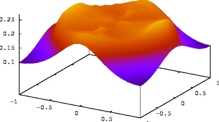
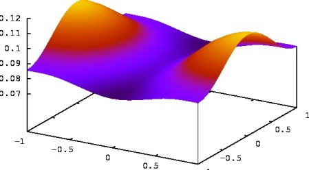
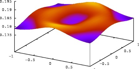
Figure 5: (color online) Representative orbital spin susceptibilities. In the basal plane, the axis on the left (longer in perspective) is $q_{x}$ axis, and the one on the right (shorter) is $q_{y}$ axis. (a) $\chi_{1111}^{S}$ (b) $\chi_{1133}^{S}$ (c) $\chi_{1177}^{S}$. Note that the maximum in $\chi_{1133}^{S}$ is located at $(\pi/a,0,0)$ and not at $2k_{F}$. Note the different vertical scales on the panels.

In Figure 5 some representative spin susceptibilities in the orbital representation are plotted on the two-dimensional basal plane ($q_{z}=0$) in the BZ. To clarify, we denote the orbitals by numbers in the order: (1)Ti₁-$d_{xy}$, (2)Ti₂-$d_{xy}$, (3)Ti₁-$d_{z^{2}}$, (4)Ti₂-$d_{z^{2}}$, (5)Ti₁-$d_{xz}$, (6)Ti₂-$d_{xz}$, (7)N₁-$p_{x}$, (8)N₂-$p_{x}$. The largest spin susceptibility is found for $\chi_{1111}^{S}$ (intersite, $xy\leftrightarrow xy$) which has approximate 4-fold symmetry for magnetic fluctuations of the same orbital $d_{xy}$ on Ti sites. The anisotropic behavior of $\chi_{1133}^{S}$ (on-site, $xy\leftrightarrow z^{2}$) comes from the orthorhombic symmetry of the lattice, i.e. $a\neq b$, which brings in anisotropic $\mathbf{q}$-dependence, in this case strongly so. The spin fluctuations between $d$ and $p$ orbitals $\chi_{1177}^{S}$ have a sizable overall magnitude, comparable to $d-d$ fluctuation, but small variation with $\mathbf{q}$, because four neighboring N atoms have almost the same distance to Ti. Due to the lack of Fermi surface nesting, there is no divergent behavior in the spin susceptibility, presenting different physics from the $\beta$-HfNCl which has two circular Fermi surfaces located at two high-symmetry (K) points in the BZ which can provide near perfect nesting.

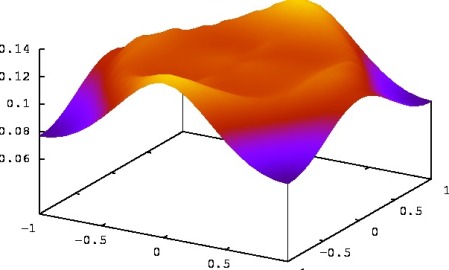
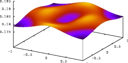
Figure 6: (color online) Representative charge susceptibilities in the full Brillouin zone. (a) $\chi_{1111}^{C}$ (b) $\chi_{1177}^{C}$. The latter quantity is hardly distinguishable from its spin counterpart. Note the different vertical scales on the panels.

Representative charge susceptibilities are shown in Figure 6. Often they have similiarities to the spin susceptibilities, with comparable but somewhat smaller magnitudes. It is known that in an extended Hubbard model on a square lattice, at zero frequency, $\chi^{S}$ and $\chi^{C}$ have similar $\mathbf{q}$-dependence and only vary in magnitude.Charge-fluc-d Without the long-range Coulomb interaction, charge fluctuation will always be smaller than spin fluctuation because of the different signs in the RPA formula. The difference between $\chi^{S}$ and $\chi^{C}$ will become more apparent at non-zero $\omega$. The $\mathbf{q}$-dependence of $\chi^{C}$ is similar to that of $\chi^{S}$ but shows somewhat more structure in $\chi_{1111}^{C}$. Note that the magnitude of $\chi_{1111}^{C}$ is only half that of $\chi_{1111}^{S}$. The spin and charge fluctuations within the N $p$-channel are very small since the $p$ orbitals are fully occupied so fluctuations only happen as a second order effect. However, the presence of the N $p$ band very close to the lowest $d$ conduction band opens an additional channel for fluctuations between them ($\chi_{1177}^{S}$, Fig. 5c and $\chi_{1177}^{C}$, Fig. 6b).

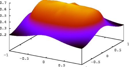
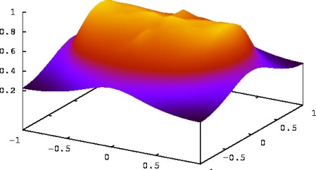
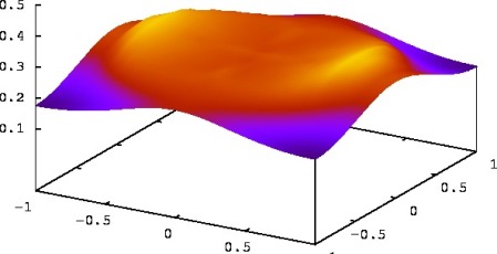
Figure 7: (color online) Macroscopic susceptibility: (a) bare; (b) spin; (c) charge. Note the strong deviation from square symmetry.

To close the comparison, we show the macroscopic susceptibilities in Figure 7. The imprint of $2k_{F}$ is evident. Beyond $2k_{F}$, the susceptibilities decrease slightly and with (near) square symmetry. Inside $2k_{F}$, the variation is greater and displays the rectangular symmetry of the lattice. The overall spin enhancement of the macroscopic susceptibility ($\chi^{S}(q)/\chi^{0}(q)$) near $\mathbf{q}=0$ is about $1.4$. For the model with the realistic parameters considered here, our test calculations show that $\chi^{S}$ will approach divergent behavior when $U\sim 4$ eV. Since TiNCl has wide $3d$ bands, it is unphysical to use $U$ anywhere near $4$ eV (we are using 1.5 eV), so strong spin fluctuation is unlikely to occur in this material. The macroscopic charge susceptibility has smaller magnitude and $\mathbf{q}$-dependence, but will show divergent behavior when inter-site interaction $V$ is much larger than $U$, but that regime is unrealistic for the case studied here. Overall, both spin and charge susceptibilities show moderate enhancements compared to the bare susceptibility, without any approach to an instability toward spin or charge ordering.

VI Conclusion

To conclude, we have constructed a many-body extended Hubbard model using a realistic band structure obtained from density functional theory calculations. RPA is applied to obtain the spin and charge susceptibilities. In a system like $\alpha$-TiNCl, where the crucial ingredients of high-temperature superconductivity, such as strong electron-phonon coupling and good Fermi surface nesting, seem to be missing, spin and charge fluctuations are the remaining candidates. Our calculations show that the spin and charge enhancements of susceptibilities, both intra-band and inter-band, are small due to moderate correlations. However, spin and charge fluctuations can produce substantial values possibly capable of encouraging electrons to pair. Although spin fluctuations are present in $\alpha$-TiNCl, it is worth pointing out that the physics is very different from the $\beta$-structure counterparts even though both are nonmagnetic, and apparently distinct from the recently discovered Fe pnictides where magnetism is an important feature in parent compounds. As the nonmagnetic nature of TiNCl and other MNX materials indicates, as well as seen from the results from our RPA calculation, charge fluctuations may have an important role in superconductivity in these systems. Overall, we still do not have a clear understanding of how superconductivity arises from the fluctuations, as with all other high-Tc families.

VII Acknowledgment

The authors would like to thank K. Kuroki and R. T. Scalettar for helpful discussions on the technical details of the RPA calculations. This work is supported by DOE Grants DE-FG02-04ER46111 and DE-FC02-06ER25794.

References

- (1) R. Weht, A. Filippetti, and W. E. Pickett, Europhys. Lett. 48, 320 (1999).
- (2) S. Yamanaka, K. Hotehama, and H. Kawaji, Nature London 392, 580 (1998).
- (3) X. Chen, T. Koiwasaki. and S. Yamanaka, J. Phys.: Condens. Matter 14, 11209 (2002).
- (4) Shoji Yamanaka, Kojiro Itoh, Hiroshi Fukuoka, and Masahiro Yasukawa, Inorg. Chem. 39, 806 (2000).
- (5) Y. Taguchi, A. Kitora, and Y. Iwasa, Phys. Rev. Lett. 97, 107001 (2006).
- (6) Hideki Tou, Yutaka Maniwa, and Shoji Yamanaka, Phys. Rev. B 67, 100509(R) (2003).
- (7) R. Heid and K.-P. Bohnen, Phys. Rev. B 72, 134527 (2005).
- (8) Shoji Yamanaka, Toshihiro Yasunaga, Kosuke Yamaguchi and Masahiro Tagawa, J. Mater. Chem. 19, 2573 (2009).
- (9) Yuichi Kasahara, Tsukasa Kishiume, Takumi Takano, Katsuki Kobayashi, Eiichi Matsuoka, Hideya Onodera, Kazuhiko Kuroki, Yasujiro Taguchi, and Yoshihiro Iwasa, Phys. Rev. Lett. 103, 077004 (2009).
- (10) T. Takano, T. Kishiume, Y. Taguchi, and Y. Iwasa, Phys. Rev. Lett. 100, 247005 (2008).
- (11) Y. Taguchi, M. Hisakabe, and Y. Iwasa, Phys. Rev. Lett. 94, 217002 (2005).
- (12) K. Kuroki, Sci. Tech. Adv. Mater. 9, 044202 (2008).
- (13) A. Bill, H. Morawitz, and V. Z. Kresin, Phys. Rev. B 66, 100501(R) (2002).
- (14) A. Bill, H. Morawitz, and V. Z. Kresin, Phys. Rev. B 68, 144519 (2003).
- (15) Masahito Mochizuki, Youichi Yanase, and Masao Ogata, Phys. Rev. Lett. 94, 147005 (2005).
- (16) Yasuhiro Tanaka , Yoichi Yanase, Masao Ogata, Physica B 359–361, 591 (2005).
- (17) Jaime Merino and Ross H. McKenzie, Phys. Rev. Lett. 87, 237002 (2001).
- (18) F. Bucci, C. Castellani, C. Di Castro, and M. Grilli, Phys. Rev. B 52, 6880 (1995).
- (19) Y. M. Vilk, Liang Chen, and A. M. S. Tremblay, Phys. Rev. B 49, 13267 (1994).
- (20) W. E. Pickett, J. Supercond. & Novel Magn. 19, 291 (2006).
- (21) Munehiro Azami, Akito Kobayashi, Tamifusa Matsuura, Yoshihiro Kuroda, Physica C 259, 227 (1996).
- (22) Y. Taguchi, T. Kawabata, T. Takano, A. Kitora, K. Kato, M. Takata, and Y. Iwasa, Phys. Rev. B 76, 064508 (2007).
- (23) H. Tou, Y. Maniwa, T. Koiwasaki, and S. Yamanaka, Phys. Rev. Lett. 86, 5775 (2001).
- (24) Tomoaki Takasaki, Toshikazu Ekino, Hironobu Fujii and Shoji Yamanaka, J. Phys. Soc. Japan 74, 2586 (2005).
- (25) T. Ekino, T. Takasaki, H. Fujii, and S. Yamanaka, Physica C 388-389, 573 (2003).
- (26) T. Ekinoa, T. Takasaki, T. Muranaka, H. Fujii, J. Akimitsu, S. Yamanaka, Physica B 328, 23 (2003).
- (27) Shoji Yamanaka, Annu. Rev. Mater. Sci. 30, 53 (2000).
- (28) K. Koepernik and H. Eschrig, Phys. Rev. B 59, 1743 (1999).
- (29) J. P. Perdew, K. Burke, and M. Ernzerhof, Phys. Rev. Lett. 77, 3865 (1996).
- (30) Kazuhiko Kuroki, Hidetomo Usui, Seiichiro Onari, Ryotaro Arita, and Hideo Aoki, Phys. Rev. B 79, 224511 (2009).
- (31) Izumi Hase and Yoshikazu Nishihara, Phys. Rev. B 60, 1573 (1999).
- (32) Izumi Hase and Yoshikazu Nishihara, Physica B 281&282, 788 (2000).
- (33) S. Yamanaka, L. Zhua, X. Chena, H. Tou, Physica B 6–9, 328 (2003).
- (34) Haruka Sugimoto and Tamio Oguchi, J. Phys. Soc. Jpn. 73, 2771 (2004).
- (35) Khee-Kyun Voo and W. C. Wu, Jian-Xin Li and T. K. Lee, Phys. Rev. B 61, 9095 (2000).
- (36) J. K. Jain and P. B. Allen, Phys. Rev. B 32, 997 (1985)