A consequence of the repulsive Casimir-Lifshitz force on nano-scale and the related Wheeler propagator in the classical electrodynamics

Abstract

Mainly on nano-scale, but maybe not exclusively, it can be imagined a spontaneous charge disjunction inside certain media due to the fluctuations, collisions, wall effects, radiation or/and other presently unknown interactions. The repulsive Casimir-Lifshitz force may be also a good candidate as a source of this kind of phenomenon. To cover this assumption mathematically an additional term should appear in the Maxwell equations. As a consequence of this term, similar Klein-Gordon equations with a negative mass term will be obtained for the electric and magnetic fields. These equations may have tachyonic solutions depending on the parameter of the charge disjunction process. Finally, the propagator is formulated, the electric field and the charge density are calculated during the charge disjunction.

1 Introduction

In the present paper the whole description remains within the framework of the classical electrodynamics. We assume that there are no net external currents and charges, i.e., if there are currents and charges these appear as a consequence of the internal processes inside the electric conductive medium. Assumable, the source of the mentioned processes maybe fluctuations, collisions, wall interactions, thermal effects, radiation. Presently, just as an interesting idea we may imagine this charge disjunction due to a repulsive Casimir-Lifshitz(-like) force [1, 2]. If we accept this possibility we should add a term in the Maxwell equations to establish the relevant mathematical equations. The calculation shows that a Klein-Gordon equation with a negative mass term will be obtained for both the electric and the magnetic field. There have been pointed out in a previous paper [3] that applying Feynman’s and Wheeler’s ideas to create the so-called Wheeler propagator, and the mathematical tools and steps ingeniously developed by Bollini, Rocca and Giambiagi [4, 5, 6, 7, 8, 9] based on the Bochner’s theorem [10, 11] we can find the propagator for a similar field equation, namely, for the Lorentz invariant thermal energy propagation [3, 12]. Since, the present mathematical equations for the electric and magnetic fields apart from the parameters are completely the same thus the mathematical elaboration is also the same. Consequently, we can obtain the causal propagator of the electromagnetic process and finally we calculate the electric field to demonstrate how the charge density increases in time.

2 Repulsive Casimir-Lifshitz force in the electrodynamics

In the present calculations we can assume that a repulsive Casimir-Lifshitz(-like) force [1, 2] may cause this kind of charge motion. The spontaneous polarization process starts at $t_{0}$ and ends $t$, and the time ${\tau}=t-t_{0}$ is really very short. The aim is to formulate those kind of equations of motion that preserve the Lorentz invariance of the theory and finally the description shows the charge disjunction. We start from the Maxwell equations modifying the second one (Eq. (1b)) with an additional term.

$$\frac{1}{{\mu}_{0}}curl{\bf B}={\varepsilon}_{0}\frac{\partial{\bf E}}{{\partial}t}+{\bf J},$$ (1a)

$$curl{\bf E}=-\frac{\partial{\bf B}}{{\partial}t}+{\alpha}^{2}\int_{t_{0}}^{t}{\bf B}({\bf r},t^{\prime})dt^{\prime},$$ (1b)

$${\varepsilon}_{0}div{\bf E}={\varrho},$$ (1c)

$$div{\bf B}=0.$$ (1d)

At this point, maybe, this step is not obvious, but it will be shown that the third term in Eq. (1b) generates the charge disjunction. This process can be considered as the consequence of an internal repulsive interaction similarly to the repulsive Casimir-Lifshitz force [1, 2]. In order to solve these equations the vector potential ${\bf A}$ is introduced by the help of Eq. (1d) as

$${\bf B}=curl{\bf A}.$$ (2)

Substituting this in to Eq. (1b) and rearranging the obtained formula we get

$$curl\left({\bf E}-\frac{\partial{\bf A}}{{\partial}t}-{\alpha}^{2}\int_{t_{0}}^{t}{\bf A}({\bf r},t^{\prime})dt^{\prime}\right)=0.$$ (3)

We can express the electric field ${\bf E}$ from the above equation

$${\bf E}=-\frac{\partial{\bf A}}{{\partial}t}-grad\,{\varphi}+{\alpha}^{2}\int_{t_{0}}^{t}{\bf A}({\bf r},t^{\prime})dt^{\prime},$$ (4)

where we introduces the scalar potential $\varphi$. We note that this formula is not Lorentz invariant, however, this fact will not cause serious problem in the description since the primary field variables are the vector and scalar potentials $A_{\mu}=({\varphi},{\bf A})$. Now, we take Eq. (1c) and we replace ${\bf E}$ into it, thus we can write

$$div{\bf E}=-\frac{{\partial}(div{\bf A})}{{\partial}t}-{\Delta}\varphi+{\alpha}^{2}\int_{t_{0}}^{t}div{\bf A}({\bf r},t^{\prime})dt^{\prime}=\frac{\varrho}{{\varepsilon}_{0}}.$$ (5)

We apply the Lorentz gauge taking ${\varepsilon}_{0}{{\mu}_{0}}=1$

$$\frac{\partial\varphi}{{\partial}t}+div{\bf A}=0,$$ (6)

we can eliminate the vector potential in Eq. (5), thus we obtain

$$\frac{{\partial}^{2}\varphi}{{\partial}t^{2}}-{\Delta}\varphi-{\alpha}^{2}\varphi=\frac{\varrho}{{\varepsilon}_{0}}.$$ (7)

This is a Lorentz invariant Klein-Gordon equation with negative mass term. Its structure is similar to the equation in Refs. [3, 12] that describes a dynamical phase transition as a consequence of a spinodal instability. The construction of Wheeler propagator is originated from the similar group of phenomena, the interaction of the radiation and the absorbing media [4, 13, 14].
The equation for the vector potential can be also formulated, starting from Eq. (1a) and substituting the form of electric field from Eq. (4)

$$curl\,curl{\bf A}=-\frac{{\partial}^{2}{\bf A}}{{\partial}t^{2}}-\frac{{\partial}grad\varphi}{{\partial}t}+{\alpha}^{2}{\bf A}+{\mu}_{0}{\bf J}.$$ (8)

Applying the vector identity $curl\,curl=grad\,div-\Delta$ and the Lorentz gauge in Eq. (6) we can rewrite the above equation in a more expressive form

$$\frac{{\partial}^{2}{\bf A}}{{\partial}t^{2}}-{\Delta}{\bf A}-{\alpha}^{2}{\bf A}={\mu}_{0}{\bf J},$$ (9)

which is also a Lorentz invariant Klein-Gordon equation with a negative mass term for the vector potential. Both the scalar and the vector potentials as basic fields – the components of a four vector $A_{\mu}=({\varphi},{\bf A})$ – fulfill Lorentz invariant equations with the same structure, they propagates with the same speed, thus the whole description is Lorentz invariant.

Now, we should write the equations for the field variables ${\bf E}$ and ${\bf B}$. Thus, we take the time derivative of Eq. (1a)

$$curl\frac{{\partial}\bf B}{{\partial}t}=\frac{{\partial}^{2}{\bf E}}{{\partial}t^{2}}+{\mu}_{0}\frac{{\partial}{\bf J}}{{\partial}t}.$$ (10)

The term of the left hand side can be substituted after the rotation of Eq. (1b) by which we write

$$curl\left(-curl{\bf E}+{\alpha}^{2}\int_{t_{0}}^{t}{\bf B}({\bf r},t^{\prime})dt^{\prime}\right)=\frac{{\partial}^{2}{\bf E}}{{\partial}t^{2}}+{\mu}_{0}\frac{{\partial}{\bf J}}{{\partial}t}.$$ (11)

We can eliminate the field ${\bf B}$ applying again Eq. (1a), and finally we obtain

$$\frac{{\partial}^{2}{\bf E}}{{\partial}t^{2}}-\Delta{\bf E}-{\alpha}^{2}{\bf E}=-\frac{1}{{\varepsilon}_{0}}grad\,{\varrho}-{\mu}_{0}\frac{{\partial}{\bf J}}{{\partial}t}+{\mu}_{0}{\alpha}^{2}\int_{t_{0}}^{t}{\bf J}({\bf r},t^{\prime})dt^{\prime}.$$ (12)

Similarly, for the field ${\bf B}$, we take the time derivative of Eq. 1b)

$$curl\frac{{\partial}{\bf E}}{{\partial}t}=-\frac{{\partial}^{2}{\bf B}}{{\partial}t^{2}}+{\alpha}^{2}{\bf B},$$ (13)

and eliminating the field ${\bf E}$ by the help of the rotation of Eq. (1a) we get

$$\frac{{\partial}^{2}{\bf B}}{{\partial}t^{2}}-\Delta{\bf B}-{\alpha}^{2}{\bf B}={\mu}_{0}curl\,{\bf J}.$$ (14)

It can be seen that for all of the field equations, Eqs. (7), (9), (12) and (14), have the same structure. We know from former studies [12, 15] that these Klein-Gordon equations with a negative mass term are resulted from repulsive interactions. Thus it seems to us that the interaction in the present case is a repulsive Casimir-Lifshitz(-like) force which appears mathematically in the second Maxwell-equation, in Eq. (1b).

3 The Wheeler propagator and the time-evolution of the electric field

Now, we can examine the appearing electrical field due to the charge disjunction given by Eq. (12). Since the last two terms of this equation make rather complicated the solution and assuming that the contribution of the current and the time derivative of the current can be negligible somehow, mainly in the initial time, we cut the right hand side to simplify the problem to

$$\frac{{\partial}^{2}{\bf E}}{{\partial}t^{2}}-\Delta{\bf E}-{\alpha}^{2}{\bf E}=-\frac{1}{{\varepsilon}_{0}}grad\,{\varrho}.$$ (15)

We solve this equation applying the Green function method, thus the electric field ${\bf E}$ can be expressed

$${\bf E}({\bf r},t)=\int-\frac{1}{{\varepsilon}_{0}}grad{\varrho}(x^{\prime})\left[\frac{1}{(2{\pi})^{4}}\int d^{4}k\frac{e^{ik(x-x^{\prime})}}{k^{2}-{\alpha}^{2}}\right]dx^{\prime},$$ (16)

where the expression

$$G(x,x^{\prime})=\frac{1}{(2{\pi})^{4}}\int d^{4}k\frac{e^{ik(x-x^{\prime})}}{k^{2}-{\alpha}^{2}}$$ (17)

in the $\left[...\right]$ bracket is the Green function. (Here, the coordinate $x=(r,t)$ involves both the space and time coordinates.) The physical description of the propagator is based on Feynman’s and Wheeler’s original idea [13, 14], the mathematical method to elaborate the calculations applying the Bochner’s theorem [10, 11] is developed by Bollini, Rocca and Giambiagi [4, 5, 6, 7, 8, 9]. Considering these preliminaries the solution of Eq. (17) in the present case is completely similar to the solution of Eq. (15) in Ref. [3] with the obvious difference that there we need to write $\alpha$ instead of $m$, and the connection ${\alpha}=\sqrt{{\mu}_{0}S_{p}}$ must be applied [16, 17] to obtain the Wheeler propagator $(n=4)$

$$W^{(4)}(x)=\frac{{\alpha}}{8\pi}(x_{0}^{2}-r^{2})_{+}^{-\frac{1}{2}}I_{-1}\left({\alpha}(x_{0}^{2}-r^{2})_{+}^{\frac{1}{2}}\right),$$ (18)

by the notations

$$x_{+}^{\beta}=x^{\beta}\;\;\;for\;\;\;x>0,$$

$$x_{+}^{\beta}=0\;\;\;for\;\;\;x<0.$$

The above propagator fulfill the requirement of causality. Finally, we can express the electric field ${\bf E}({\bf r},t)$ by the calculated propagator

$${\bf E}({\bf r},t)=\int-\frac{1}{{\varepsilon}_{0}}grad{\varrho}(x^{\prime})W^{(4)}(x-x^{\prime})dx^{\prime}$$ (19)

as a four dimensional convolution. Probably, the spontaneous polarization cannot be detected directly but there may be several consequences of it. The demonstration of the phenomenon seems rather difficult because there is no freely propagating particle during the excitation.

4 Evolution of a nearly flat Gaussian charge distribution

On the basis of the previous calculations we expect that a small perturbation can grow up to a huge dipole pair within the short time $\tau$, and it disappears similarly fast. As an example we examine the time evolution of a Gaussian charge distribution

$${\varrho}(x)={\varrho}_{0}e^{-ar^{2}}\delta(t-t_{0}).$$ (20)

If the parameter $a\sim 0$, the charge distribution can be considered practically homogeneous $(e^{-ar^{2}}\sim 1)$. The time-dependent factor have a sharp peak if $\epsilon$ tends to zero. So, if we consider the charge gradient for small values of $a$ and $\epsilon$ we obtain

$$grad\,\varrho(x)=-2{\varrho}_{0}a\delta(t){\bf r}e^{-ar^{2}}\,\sim\,-2{\varrho}_{0}a\delta(t-t_{0}){\bf r}.$$ (21)

Here, we apply the ”early” form of the Wheeler propagator [see Eq. (32) in Ref. [3]]

$$W(x)=\frac{Sgn(x_{0})}{16\pi^{3}}\int\limits_{-\infty}^{\infty}\frac{\sin(p^{2}-\alpha^{2}+i0)^{\frac{1}{2}}x_{0}}{(p^{2}-\alpha^{2}+i0)^{\frac{1}{2}}}e^{i{p}\cdot{x}}d^{3}p$$ (22)

for the further calculations. Substituting the charge gradient in Eq. (21) and the Wheeler propagator in Eq. (22) into the expression of Eq. (19) then we obtain the time evolution of the electric field

$${\bf E}(x)=\frac{2\varrho_{0}a}{16\pi^{3}\varepsilon_{0}}Sgn(t-t_{0})\int\limits_{-\infty}^{\infty}\frac{\sin(p^{2}-\alpha^{2}+i0)^{\frac{1}{2}}(t-t_{0})}{(p^{2}-\alpha^{2}+i0)^{\frac{1}{2}}}e^{i{p}\cdot({x}-{x}^{\prime})}{x}^{\prime}\;d^{3}p\;d^{3}x^{\prime}.$$ (23)

After the evaluation of the integral ans simplifying the mathematical expression the electric field can be analytically expressed

$${\bf E}(x)=\frac{\varrho_{0}a}{\varepsilon_{0}}{\bf r}\;Sgn(t-t_{0})\frac{\sin(-{\alpha}^{2}+i0)^{\frac{1}{2}}(t-t_{0})}{(-{\alpha}^{2}+i0)^{\frac{1}{2}}}=$$

$$\frac{\varrho_{0}a}{\varepsilon_{0}\alpha}{\bf r}\sinh(\alpha|t-t_{0}|)\,\sim\,\frac{\varrho_{0}a}{\varepsilon_{0}\alpha}{\bf r}e^{-ar^{2}}\sinh(\alpha|t-t_{0}|)$$ (24)

It can be read out easily from this exact result that the magnitude of the electric field ${\bf E}$ follows an exponential behavior. The source of the huge electric field is the enormously growing charge distribution

$${\varrho}(r,t)=\frac{\varrho_{0}a}{\alpha}(3-2ar^{2})e^{-ar^{2}}\sinh(\alpha|t-t_{0}|)\,\sim\,3\frac{\varrho_{0}a}{\alpha}e^{-ar^{2}}\sinh(\alpha|t-t_{0}|),$$ (25)

which can be obtained by the Maxwell equation $div{\bf E}={\varrho}/{\varepsilon_{0}}$. It is interesting to see that if we integrate this charge density for the whole space the result is always zero for all positive values of the parameter $a>0$

$$\int_{0}^{\infty}{\varrho}(r,t)dV=4{\pi}\int_{0}^{\infty}\frac{\varrho_{0}a}{\alpha}r^{2}(3-2ar^{2})e^{-ar^{2}}\sinh(\alpha|t-t_{0}|)\;dr=0,$$ (26)

i.e., the conservation law of electric charge is completed, there is only internal movement of the charges – charge disjunction. Applying the continuity relation

$$\frac{\partial\varrho}{{\partial}t}+div\,{\bf J}=0,$$ (27)

and considering Eqs. (1c) and (24) we obtain the current ${\bf J}$

$${\bf J}=-{\varrho}_{0}\,a\,{\bf r}e^{-ar^{2}}Sgn(t-t_{0})\cosh(\alpha|t-t_{0}|)\,\sim\,-{\varrho}_{0}\,a\,{\bf r}\,Sgn(t-t_{0})\cosh(\alpha|t-t_{0}|).$$ (28)

Here, we note that calculating the dropped part of Eq. (12)

$$-{\mu}_{0}\frac{{\partial}{\bf J}}{{\partial}t}+{\mu}_{0}{\alpha}^{2}\int_{t_{0}}^{t}{\bf J}({\bf r},t^{\prime})dt^{\prime}$$ (29)

with the above solution of the current in Eq. (28), we obtain zero. (The initial condition for the current: at time $t_{0}$ the current ${\bf J}=0$.) Thus, we can say that the obtained solution for the electric field in Eq. (24) and the for the charge density in Eq. (25) from the cut Klein-Gordon equation in Eq. (15) can be considered as exact results.

The above results clearly show that – let us say – the positive charges are moving towards the origin, and reversely, the negative charges are moving towards the radius $r=1.5$. Of course, the sign of the charges may be opposite. Naturally, the process must be restricted to nano-distances. Furthermore, the process stops after the very short time $\tau$, and it turns back, so finally the system reaches its originally homogeneous charge distribution again. The present calculations does not involve the possibility of a charge oscillations, but this process may be also realistic. This examination and discussion are challenges for a future work.

The time evolution of the charge density is shown in Fig. 1. Since the physical situation is spherically symmetric it is enough to demonstrate the increase of the charge density as a function of the radius $r$ in different time moments.

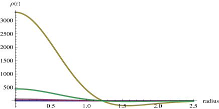
Figure 1: Charge densities as a function of the radius $r$ in three different time moments: $t=0.3$ (purple line – below), $t=0.6$ (green line – middle), $t=0.8$ (grey line – above). The charge density and time are in arbitrary units.

This figure demonstrates spectacularly how fast the charge density increases in time. The parameters can be taken optionally at the present stage, thus ${\varrho}_{0}=1,a=1$ and ${\alpha}=10$, which means that the scale is arbitrary on the figure. We can see that at the beginning the charge density increases rather slowly comparing the later time, and in a certain time it can grow up in a giant form. During the elapsing time a negative spherically symmetric charge density is collecting with a maximal value at the radius $r=1.5$. The process stops at the very short time $\tau$, and it turns back, so finally the system reaches its originally homogeneous charge distribution.

5 Summary

In the present work it is pointed out that an assumed repulsive Casimir-Lifshitz-like force may cause a giant charge disjunction on a short range within a short time. Inspite of the related causal Wheeler propagator, probably, these excited particles are hidden non-observable entities. However, if this process may happen, it may contribute to the physical behavior of some small systems, e.g. on nano-scale to the electric properties or other transport phenomena of few body systems.

6 Acknowledgment

The authors would like to thank the National Office of Research and Technology (NKTH; Hungary) for financial support MX-20/2007 (Grant No. OMFB-00960/2008). This work is connected to the scientific program of the ” Development of quality-oriented and harmonized R+D+I strategy and functional model at BME” project. This project is supported by the New Hungary Development Plan (Project ID: T?MOP-4.2.1/B-09/1/KMR-2010-0002).

References

- [1] J. N. Munday, F. Capasso and V. A. Parsegian, Nature 457, 170 (2009).
- [2] S. K. Lamoreaux, Nature 457, 156 (2009).
- [3] F. Márkus and Gambár, Int. J. Theor. Phys. 49, 2065 (2010).
- [4] C. G. Bollini, L. E. Oxman and M. C. Rocca, Int. J. Theor. Phys. 38, 777 (1999).
- [5] C. G. Bollini and M. C. Rocca, Int. J. Theor. Phys. 37, 2877 (1998).
- [6] C. G. Bollini and J. J. Giambiagi, Phys. Rev. D 53, 5761 (1996).
- [7] C. G. Bollini and M. C. Rocca, Int. J. Theor. Phys. 43, 1019 (2004).
- [8] C. G. Bollini and M. C. Rocca, Nuovo Cimento A 110, 353 (1997).
- [9] C. G. Bollini and M. C. Rocca, Nuovo Cimento A 110, 363 (1997).
- [10] S. Bochner, Lectures on Fourier Integrals (Princeton Univ., New Jersey, 1939), p. 235.
- [11] A. J. Jerri, The Gibbs Phenomenon in Fourier Analysis, splines, and wavelet approximations (Kluwer, Dordrecht, 1998).
- [12] K. Gambár and F. Márkus, Phys. Lett. A 361, 283 (2007).
- [13] J. A. Wheeler and R. P. Feynman, Rev. Mod. Phys. 17, 157 (1945).
- [14] J. A. Wheeler and R. P. Feynman, R.P: Rev. Mod. Phys. 21, 425 (1949).
- [15] K. Gambár and F. Márkus, Rep. Math. Phys. 62, 219 (2008).
- [16] The Wheeler propagator in the dimensional space-time is (see in Ref. [3])
- [17] S. Gradshteyn and I. M. Ryzhik, Tables of Integrals, Series, and Products (Academic Press, New York, 1994).