Optical scattering by a nonlinear medium, II: induced photonic crystal in a nonlinear slab of BBO

Abstract

The purpose of this paper is to investigate the scattering by a nonlinear crystal whose depth is about the wavelength of the impinging field. More precisely, an infinite nonlinear slab is illuminated by an incident field which is the sum of three plane waves of the same frequency, but with different propagation vectors and amplitudes, in such a way that the resulting incident field is periodic. Moreover, the height of the slab is of the same order of the wavelength, and therefore the so-called slowly varying envelope approximation cannot be used. In our approach we take into account some retroactions of the scattered fields between them (for instance, we do not use the nondepletion of the pump beam). As a result, a system of coupled nonlinear partial differential equations has to be solved. To do this, the finite element method (FEM) associated with perfectly matched layers is well suited. Nevertheless, when using the FEM, the sources have to be located in the meshed area, which is of course impossible when dealing with plane waves. To get round this difficulty, the real incident field is simulated by a virtual field emitted by an appropriate antenna located in the meshed domain and lying above the obstacle (here the slab).

1 Introduction

The development of photonic science in nanotechnologies requires an always increasing control of light. Surface-phenomena, metamaterials or the use of nonlinear optics are very efficient ways to do this. In this paper, we combine the last two options: an electromagnetic field induces, in a homogeneous nonlinear medium, a periodicity of period close to the considered wavelength. A precise description of the system is given in the next section.

The majority of work in nonlinear optics applies to the propagation of a wave in a nonlinear medium (see [1] for a review), that is, the wavelength is small compared to the length of the path of light in the nonlinear medium. In this case, the paraxial approximation is often used and the equations obtained are of parabolic kinds. For example, when studying the propagation of a soliton in an optical fiber (say, oriented along the $z$-axis), one usually restrict the problem in the $(z,t)$-plane, neglecting the transversal effects. This leads to equations of the nonlinear Schrödinger type. Some works have been done to determine the limits of this approach ([2, 3, 4]). This justifies the studies done directly with Maxwell’s equations, as in [5, 6], where transversal effects are taken into account.

On the other side, when the wavelength is far larger than the obstacle, a mean-field approximation is used ([7, 8]). The purpose of this paper is to stand between these two states, in the realm of resonance, where rough approximations cannot be applied. To this end, we use the FEM: the precision in the change of apparent permittivity inside the slab (i.e., the inhomogeneity of the sources, resonating with different frequencies, of the total field) is only dictated by the memory size of the computer.

The study of nonlinear optics in periodic material is of course not new ([9, 10], see also [11]). It is known that Kerr photonic crystals allow to produce systems with hysteresis ([7, 12]), or with a transmission range that depends on the amplitude of the fields ([13, 14]). Peak of transmission can also appear in the gap due to the nonlinearity ([15, 16]).

When considering harmonic generation due to a nonlinear periodic structure, the phenomena that appear in photonic crystals are still richer, for the frequency components of the fields can have completely different behaviors ([17, 18, 19, 20]).

Finally, this paper also aims at exposing an application of the companion paper [21], that gives a new route to obtain propagation equations in nonlinear optics.

2 Set up of the problem

2.1 Description of the system

The choice of the test structure has been dictated by two guidelines: it must be at the same time simple enough to lead to tractable numerical models and possibly feasible experiments, and enhance the nonlinear effects both qualitatively and quantitatively. For this, we propose the following experiment: let three plane waves impinge on a slab, made up of a nonlinear and non-centro-symmetric crystal. One wave is directed normally with respect to the slab, the other two are symmetrically oriented with respect to it and have the same amplitude (the analytical expression of the incident field is given in subsection 3.1). In this way, the problem is periodic, along one direction that we call the $x$-axis. This incident field create an optical lattice ([22, 23]), as seen in the figure 1. Hence, the scattered field presents several orders of reflection and of transmission. Furthermore, the scattered field oscillate at several pulsations, due to harmonic generation in the crystal. The range of ratios wavelength/period of the crystal offers a variety of response for the different harmonics. In particular, the smaller the wavelength, the more order excited. This implies that there are more scattered angles for the fields oscillating at the generated harmonics than for the one oscillating at the incident frequency. Moreover, and we find it spectacular, the energy that flows along each direction of the crystal is not at all a monotonous function of the incident intensity. This offers new ways to control the directions along which the higher harmonics escape from the nonlinear medium.

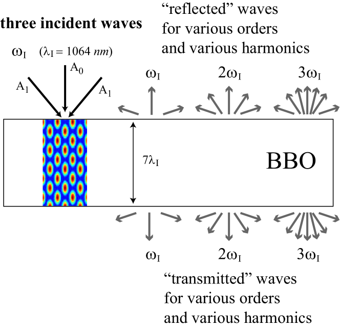
Figure 1: The geometry of the system is a slab, invariant along the horizontal direction, called the $x$ axis, and along the direction perpendicular to the plane of the sheet of paper, called the $z$ axis. Made up of $\beta$ Barium Borate (BBO), it is illuminated by three plane waves: one with a normal incidence and an amplitude $A_{0}$, and two with a symmetric oblique incidence and amplitude $A_{1}$. The interferences between these different incident waves oscillating at $\omega_{I}$, induces a periodic structure, equivalent to a diffraction grating or a finite photonic crystal. This is seen in color inside the slab, where the pattern of the intensity field $\|\mathbf{E}_{1}^{i}\|$ of the incident waves is shown. This nonlinear induced grating generate some harmonics. The number of propagating order increases with the pulsation. (Three periods are presented in this picture, though the simulation runs with one period only.)

Let $\lambda_{I}$ be the wavelength of the incident field. The slab we choose had a thickness of $7.06\ \lambda_{I}$. In this range, the slowly varying envelop is not a good approximation, so we have to solve the complete set of Maxwell’s equations. But, as shown in [21], Maxwell’s equations lead to an infinite set of nonlinear and coupled equations. The article just mentioned is mainly devoted to the elaboration of this system, and then its truncation, necessary for a numerical study. Some results are briefly reminded in the following subsection; the reader is reported to [21] for their justification.

2.2 What kind of equations has to be solved?

We consider a spatially local, nonbianisotropic, stationary, magnetically linear, smooth medium (see [21] for a definition; the idea behind a smooth medium is that we can make a Taylor expansion of the electric induction field in function of the electric field). For simplicity, the electric susceptibility tensor $\chi^{(n)}$ are neglected when $n>3$. The nonlinear effects we want to consider are mainly the second and third harmonic generations. Hence the nonharmonic processes (like Raman or Brillioun scatterings) are not taken into account.

We write the electric vector, at a point $\mathbf{s}$ and a time $t$ as

$$\mathbf{E}(\mathbf{s},t)=2\Re\it{e}\{\mathbf{E}_{1}(\mathbf{s})e^{-i\omega_{I}t}+\mathbf{E}_{2}(\mathbf{s})e^{-2i\omega_{I}t}+\mathbf{E}_{3}(\mathbf{s})e^{-3i\omega_{I}t}\}.$$

Note that this expression implies that we neglect the cascading effect that create harmonics higher than the third one; also, as it is often the case, the static component is supposed to vanish.

To write the propagation equations, we need to introduce two notations: the first one is the operator $\mathcal{M}_{p}^{lin}$, that, when applied to the $p$-th component $\mathbf{E}_{p}$ of the electric field, gives the equation satisfied by $\mathbf{E}_{p}$ in a linear medium; the second one is a short way of writing the interactions between several components of the total electric field. For example, $\lfloor\mathbf{E}_{1},\mathbf{E}_{1}\rfloor:=\chi^{(2)}(\omega_{I},\omega_{I})\mathbf{E}_{1}\mathbf{E}_{1}$, describes the interaction of $\mathbf{E}_{1}$ with itself - this term is the source of the second harmonic generation -, $\lfloor\mathbf{E}_{-1},\mathbf{E}_{1},\mathbf{E}_{1}\rfloor:=\chi^{(3)}(-\omega_{I},\omega_{I},\omega_{I})\mathbf{E}_{-1}\mathbf{E}_{1}\mathbf{E}_{1}$, is the term that describes the interaction between $\mathbf{E}_{-1}$, $\mathbf{E}_{1}$ and $\mathbf{E}_{1}$. Since $\mathbf{E}_{-p}=\overline{\mathbf{E}_{p}}$, this is precisely the optical Kerr effect. More formally, we have

$$\mathcal{M}_{p}^{lin}(\mathbf{E}_{p}):=-\varepsilon_{0}^{-1}\nabla\times(\mu^{-1}(p\omega_{I})\nabla\times\mathbf{E}_{p})+(p\omega_{I})^{2}\varepsilon_{r}^{(1)}(p\omega_{I})\mathbf{E}_{p}$$

and

$$\lfloor\mathbf{E}_{p_{1}},\cdots,\mathbf{E}_{p_{n}}\rfloor:=\chi^{(n)}(p_{1}\omega_{I},\cdots,p_{n}\omega_{I})\mathbf{E}_{p_{1}}\cdots\mathbf{E}_{p_{n}}$$

where $p_{i}\in\mathbb{Z}$. Note that this term contributes to the component of the $n$-th order polarization oscillating at the pulsation $(p_{1}+\cdots+p_{n})\omega_{I}$

Now, as said above, we want to study the second and third harmonic generations. Their respective sources are $\lfloor\mathbf{E}_{1},\mathbf{E}_{1}\rfloor$ for $\mathbf{E}_{2}$, and $\lfloor\mathbf{E}_{1},\mathbf{E}_{2}\rfloor$ and $\lfloor\mathbf{E}_{1},\mathbf{E}_{1},\mathbf{E}_{1}\rfloor$ for $\mathbf{E}_{3}$. Note that we consider here a cascading effect: $\mathbf{E}_{1}$ and $\mathbf{E}_{2}$ interact to create $\mathbf{E}_{3}$. In fact, we give a set of equations that allows to consider a lossless process ([21, 24]):

$$\mathcal{M}_{1}^{lin} (\mathbf{E}_{1})$$ (1a)

$$+\omega_{I}^{2}\Big{(}2\lfloor\mathbf{E}_{-2},\mathbf{E}_{3}\rfloor+2\lfloor\mathbf{E}_{-1},\mathbf{E}_{2}\rfloor$$

$$+6\lfloor\mathbf{E}_{-3},\mathbf{E}_{1},\mathbf{E}_{3}\rfloor+3\lfloor\mathbf{E}_{-1},\mathbf{E}_{-1},\mathbf{E}_{3}\rfloor+3\lfloor\mathbf{E}_{-3},\mathbf{E}_{2},\mathbf{E}_{2}\rfloor$$

$$+6\lfloor\mathbf{E}_{-2},\mathbf{E}_{1},\mathbf{E}_{2}\rfloor+3\lfloor\mathbf{E}_{-1},\mathbf{E}_{1},\mathbf{E}_{1}\rfloor\Big{)}=\mathfrak{s}(\mathbf{E}^{i}_{1}),$$

$$\mathcal{M}_{2}^{lin} (\mathbf{E}_{2})$$ (1b)

$$+(2\omega_{I})^{2}\Big{(}2\lfloor\mathbf{E}_{-1},\mathbf{E}_{3}\rfloor+\lfloor\mathbf{E}_{1},\mathbf{E}_{1}\rfloor$$

$$+6\lfloor\mathbf{E}_{-3},\mathbf{E}_{2},\mathbf{E}_{3}\rfloor+6\lfloor\mathbf{E}_{-2},\mathbf{E}_{1},\mathbf{E}_{3}\rfloor+3\lfloor\mathbf{E}_{-2},\mathbf{E}_{2},\mathbf{E}_{2}\rfloor$$

$$+6\lfloor\mathbf{E}_{-1},\mathbf{E}_{1},\mathbf{E}_{1}\rfloor\Big{)}=0,$$

$$\mathcal{M}_{3}^{lin} (\mathbf{E}_{3})$$ (1c)

$$+(3\omega_{I})^{2}\Big{(}2\lfloor\mathbf{E}_{1},\mathbf{E}_{2}\rfloor$$

$$+3\lfloor\mathbf{E}_{-3},\mathbf{E}_{3},\mathbf{E}_{3}\rfloor+6\lfloor\mathbf{E}_{-2},\mathbf{E}_{2},\mathbf{E}_{3}\rfloor+6\lfloor\mathbf{E}_{-1},\mathbf{E}_{1},\mathbf{E}_{3}\rfloor$$

$$+3\lfloor\mathbf{E}_{-1},\mathbf{E}_{2},\mathbf{E}_{2}\rfloor+\lfloor\mathbf{E}_{1},\mathbf{E}_{1},\mathbf{E}_{1}\rfloor\Big{)}=0.$$

Note that some other interesting effects are taken into account: the optical Kerr effect ($\lfloor\mathbf{E}_{1},\mathbf{E}_{1},\mathbf{E}_{-1}\rfloor$), the depletion of the pump beam ($\lfloor\mathbf{E}_{2},\mathbf{E}_{-1}\rfloor$). On the other hand, some terms are really weak (typically $\lfloor\mathbf{E}_{3},\mathbf{E}_{3},\mathbf{E}_{-3}\rfloor$ as compared to $\lfloor\mathbf{E}_{1},\mathbf{E}_{1},\mathbf{E}_{1}\rfloor$) and do not have important consequences on the fields. The presence of these interactions is only due to the energy conservation property, which is a good test from the numerical point of view. Finally, $\mathfrak{s}(\mathbf{E}^{i}_{1})$ is the external source of $\mathbf{E}_{1}$; since in our case the slab is illuminated by plane waves, $\mathfrak{s}(\mathbf{E}^{i}_{1})$ vanishes.

3 Some Numerical Results

3.1 From a practical point of view

To solve the system of equations we posed, numerical methods have to be used. The nonlinearity is tackled by a Newton-Raphson scheme and, at each step, the finite element method was chosen for its ability to treat the nonhomogeneous sources, induced by the nonlinearity, of each equation. The incident wave is monochromatic, $\mathbf{E}^{i}(\mathbf{s},t)=2\Re\it{e}\{\mathbf{E}_{1}^{i}(\mathbf{s})e^{-i\omega_{I}t}\}$, and to simplify the comparison with an experimental setup, we fix $\omega_{I}$ such that the associated wavelength is $\lambda_{I}=1064\,nm$, which corresponds to a Nd:YAG laser.

Only two-dimensional problems are addressed here. We recall that the physical system is invariant along the $x$ and the $z$ axis. The $TH$ polarization is chosen, that is, a function $u^{i}:\mathbb{R}^{2}\rightarrow\mathbb{C}$ satisfies, in Cartesian coordinates,

$$\mathbf{E}^{i}_{1}(x,y,z)=u^{i}(x,y)\hat{z}.$$

Now a key step is described: the crystal we choose is the $\beta$ Barium Borate (from now on denoted as BBO); it is known that there exists one orientation of the crystal that guarantees that the total field has the same polarization as the incident field:

$$\mathbf{E}_{p}(x,y,z)=u_{p}(x,y)\hat{z}$$

for some functions $u_{p}:\mathbb{R}^{2}\rightarrow\mathbb{C}$. We choose this orientation, so that the $p$-th component of the electric field is described with these scalar functions.

Finally, the propagation equation system (1) being given in term of the total electric field, we use a virtual antenna to simulate the incident field ([25]). Perfectly matched layers are used to impose outgoing wave conditions above and below the slab, for $u_{1}$, $u_{2}$ and $u_{3}$. For the reader’s convenience, we give the electric current that simulates the incident electric field:

$$\mathbf{j}(x,y,t)=2\Re\it{e}\{\j(x,y)\ e^{-i\omega_{I}t}\}\hat{z},$$

with

$$\j(x,y)=\frac{1}{\mu\ \omega_{I}}\{\ kA_{0}e^{-iky}+2\beta A_{1}\ e^{-i\beta y}\cos(\alpha x)\}\delta(y-h),$$

to be evaluated at $h$, where $h$ is the height of the thread on which the current flows, $\alpha:=\mathbf{k}\cdot\hat{x}=k\sin(\theta)$ and $\beta:=\mathbf{k}\cdot\hat{y}=k\cos(\theta)$ ($k:=\|\mathbf{k}\|=2\pi/\lambda_{I}$ is common to the three incident waves and $\theta$ is the obliquity angle of the waves with the amplitude $A_{1}$), and $\delta$ is the Dirac distribution. The expression of the incident field is then

$$u^{i}(x,y)=A_{0}e^{-iky}+2A_{1}e^{-i\beta y}\cos(\alpha x).$$

3.2 Scattering Of Three Waves On A Slab

We come now to the results of the simulation of the experiment described in the figure 1. This system exhibits a non trivial and quite complex behavior because of the induced diffraction grating.

The numerical value of the relevant susceptibility components are given in the table 1.We note that they do not depend on the frequency.

$\lambda$	$n_{e}$	$\chi^{(1)\,z}_{\qquad z}$	$\chi^{(2)\,z}_{\qquad zz}$	$\chi^{(2)\,z}_{\qquad zzz}$
$1064$	$1.5426$	$1.3793$	$2.10^{-12}$	$10^{-23}$
$532$	$1.5555$	$1.4196$	$2.10^{-12}$	$10^{-23}$
$355$	$1.5775$	$1.4885$	$2.10^{-12}$	$10^{-23}$

Table 1: The wavelength, in $nm$, the refraction index of the extraordinary axis, and the values of the relevant (in that article) $\chi^{(1)}$, $\chi^{(2)}$ and $\chi^{(3)}$, respectively without unit, in $m.V^{-1}$ and in $m^{2}.V^{-2}$.

We are interested in the directions where the fields scatter. Out of the slab, for each frequency, the electric field satisfies a Helmholtz equation. We write its propagating solution as

$$\mathbf{E}_{p}(x,y) =\sum_{n\in\mathcal{U}_{p}}\{b^{(r)}_{p,n}e^{i\big{(}\frac{2\pi n}{d}x+(k_{p}^{2}-(\frac{2\pi n}{d})^{2})^{1/2}y\big{)}}$$

$$\quad+b^{(t)}_{p,n}e^{i\big{(}\frac{2\pi n}{d}x-(k_{p}^{2}-(\frac{2\pi n}{d})^{2})^{1/2}y\big{)}}\}\hat{z},$$

where $b^{(r)}_{p,n}$ (resp. $b^{(t)}_{p,n}$) denotes the coefficient of the $n$-th order of the reflected (resp. transmitted) wave at pulsation $p\omega_{I}$, and $\mathcal{U}_{p}:=\{n\in\mathbb{Z}:k_{p}^{2}-(\frac{2\pi n}{d})^{2}>0\}$. Since $k_{p}=p\omega_{I}/c$ (where $c$ is the light velocity), the higher the harmonic $p$, the higher the modulus of the wave vector $k_{p}$; in other words, the size of $\mathcal{U}_{p}$ increases with $p$. This means that there are more scattered angles for higher harmonics than for the field oscillating at the fundamental frequency. In our particular case, whereas only the orders $-1$, $0$ and $1$ are present in $\mathbf{E}_{1}$, the third harmonic contains orders from $-3$ to $3$. These ranges depend on the wavelength and the inclination $\theta$ of the incident beams; had we chosen a larger $d$, the propagating orders allowed for the first harmonic would have ranged from, say, $-2$ to $2$.

The second thing we note is that the amplitude of the $n$-th order of the $p$-th harmonic (that is $b^{(r)}_{p,n}$ or $b^{(t)}_{p,n}$) is not monotonic in the amplitude of the incident field, as is seen in the figures 2-4 (due to the reflection symmetry along the $y$-axis of the system, $b^{(t)}_{p,-n}=b^{(t)}_{p,n}$ and $b^{(r)}_{p,-n}=b^{(r)}_{p,n}$). In the figures are represented the efficiency of the transmitted waves - the reflected ones show similar behaviors - defined by:

$$e^{(a)}_{p,n}:=\frac{|b^{(a)}_{p,n}|}{\sum_{n\in\mathcal{U}_{p}}|b^{(a)}_{p,n}|}$$

for $a\in\{r,t\}$. It thus gives the part of the intensity of the reflected or transmitted wave at pulsation $p\omega_{I}$ that escapes along the $n$-th order.

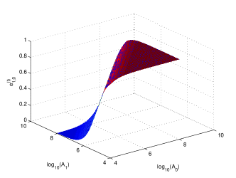
(a) $e^{(t)}_{1,0}$

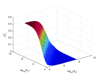
(b) $e^{(t)}_{1,1}$

Figure 2: The efficiency of the transmitted propagating waves at the frequency $\omega_{I}$. As is easily understood, when $A_{1}$ tends to zero, all the light escape perpendicularly to the slab, i.e., $e^{(t)}_{1,0}$ tends to one and $e^{(t)}_{1,1}$ vanishes.

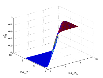
(a) $e^{(t)}_{2,0}$

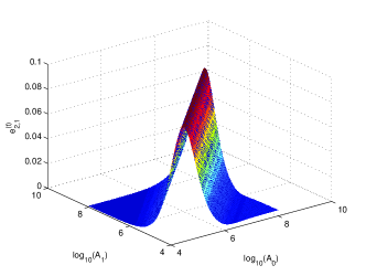
(b) $e^{(t)}_{2,1}$

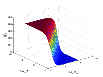
(c) $e^{(t)}_{2,2}$

Figure 3: The efficiency of the transmitted propagating waves at the frequency $2\omega_{I}$. Schematically, when $A_{0}>A_{1}$ (resp. $A_{0}\sim A_{1}$, $A_{0}<A_{1}$), the $0^{th}$ (resp. $1^{st}$, $2^{nd}$) order is favored. That $e^{(t)}_{2,1}$ is peaked around $A_{0}=A_{1}$ was a surprise for us.

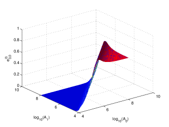
(a) $e^{(t)}_{3,0}$

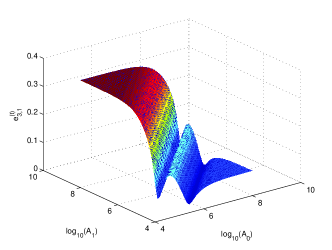
(b) $e^{(t)}_{3,1}$

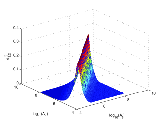
(c) $e^{(t)}_{3,2}$

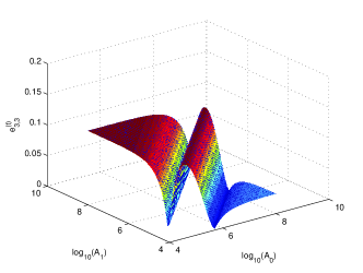
(d) $e^{(t)}_{3,3}$

Figure 4: The efficiency of the transmitted propagating waves at the frequency $3\omega_{I}$. These maps present large resonances (see the scale for $e^{(t)}_{3,2}$).

4 Concluding Remarks

We present numerical evidences that the scattering of several waves on a nonlinear slab, whose thickness is of the order of the wavelength, shows rich phenomena. This system is studied through a set of equations obtained from a rigorous method, given in a companion paper. The response of the induced grating is far from being monotonous in the amplitudes of the pump wave. We now look for an experimental test.

Aknowledgement

The authors are grateful to S. Brasselet and A. Ferrando for their comments about this manuscript.

References

- [1] Y.S. Kivshar and D.E. Pelinovsky. Self-focusing and transverse instabilities of solitary waves. Physics Report, 331:117, 2000.
- [2] Y. Chen and J. Atai. Maxwell’s equations and the vector nonlinear Schrödinger equation. Physical Review E, 55(3):3652, 1997.
- [3] A. Ciattoni, B. Crosignani, P. di Porto, and A. Yariv. Perfect optical solitons: spatial Kerr solitons as exact solutions of Maxwell’s equations. Journal of the Optical Society of America, B, 22(7):1384, 2005.
- [4] F. Drouart, G. Renversez, A. Nicolet, and C. Geuzaine. Spatial Kerr solitons in optical fibres of finite size cross section: beyond the Townes soliton. Journal of Optics A: pure and applied optics, 10:125101, 2008.
- [5] A. Ferrando, M. Zacares, P. Fernandez de Cordoba, D. Binosi, and J.A. Monsoriu. Spatial soliton formation in photonic crystal fibers. Optics Express, 11(5):452, 2003.
- [6] S.A. Darmanyan and M. Nevière. Dichromatic nonlinear eigenmodes in slab waveguide with nonlinearity. Physical Review E, 63:36613, 2001.
- [7] E. Centeno and D. Felbacq. Optical bistability in finite-size nonlinear bidimensional photonic crystals doped by a microcavity. Physical Review B, 62(12):7683, 2000.
- [8] P. Xie, Z.Q. Zhang, and Z. Zhang. Gap solitons and solitons trains in finite-sized two-dimensional periodic and quasiperiodic photonic crystals. Physical Review E, 67:026607, 2003.
- [9] N. Bloembergen and A.J. Sievers. Nonlinear optical properties of periodic laminar structures. Applied Physics Letter, 17:483, 1970.
- [10] R. Reinisch, G. Chartier, M. Nevière, M.C. Hutley, G. Clauss, J.P. Galaup, and J.F. Eloy. Experiment of diffraction in nonlinear optics: second harmonic generation by a nonlinear grating. Journal de Physique Lettres, 44:1007, 1983.
- [11] M. Nevière, E. Popov, R. Reinisch, and G. Vitrant. Electromagnetic Resonances in Nonlinear Optics. Gordon and Breach Science Publishers, 2000.
- [12] M. Soljacic, M. Ibanescu, S.G. Johnson, Y. Fink, and J.D. Joannopoulos. Optimal bistable switching in nonlinear photonic crystals. Physical Review E, 66:55601, 2002.
- [13] A. Cicek and B. Ulug. Influence of Kerr nonlinearity on the band structures of two-dimensional photonic crystals. ScienceDirect, 281:3924, 2008.
- [14] T. Fujisawa and M. Koshiba. Time-domain beam propagation method for nonlinear optical propagation analysis and its application to photonic crystal circuits. Journal of Lightwave Technology, 22(2):684, 2004.
- [15] W. Chen and D.L. Mills. Gap solitons and the nonlinear optical response of superlattices. Physical Review Letters, 58(2):160, 1987.
- [16] S. John and N. Ak zbek. Nonlinear optical solitary waves in a photonic band gap. Physical Review Letters, 71(8):1168, 1993.
- [17] R. Lifshitz, A. Arie, and A. Bahabad. Photonic quasicrystals for nonlinear optical frequency conversion. Physical Reviews Letters, 95:133901, 2004.
- [18] E. Centeno and D. Felbacq. Second-harmonic emission in two-dimensional photonic crystals. Journal of the Optical Society of America B, 23(10):2257, 2006.
- [19] M.W. Klein, M. Wegener, N. Feth, and S. Linden. Experiments on second- and third-harmonic generation from magnetic metamaterial. Optics Express, 15(8):5238, 2007.
- [20] N. Mattiucci, G. D’Aguanno, M. Scalora, and M.K. Bloemer. Coherence length for second-harmonic generation in nonlinear, one-dimensional, finite, multilayered structures. Journal of the Optical Society of America, 24(4):877, 2007.
- [21] P. Godard, F. Zolla, and A. Nicolet. Optical scattering by a nonlinear medium, I: from Maxwell equations to numerically tractable equations. to appear, 2011.
- [22] B. Freedman, G. Bartal, M. Segev, R. Lifshitz, D.N. Christodoulides, and J.W. Fleischer. Wave and defect dynamics in nonlinear photonic quasicrystals. Nature, 440:1166, 2006.
- [23] P. Zhang, R. Egger, and Z. Chen. Optical induction of three-dimensional photonic lattices and enhancement of discrete diffraction. Optics Express, 17(15):13151, 2009.
- [24] P. Godard. Optique Non-lin aire Polyharmonique : de la Théorie à la Modélisation Numérique. Editions Universitaires Européennes, 2010.
- [25] P. Godard, F. Zolla, and A. Nicolet. Scattering by a 2-dimensional doped photonic crystal presenting an optical Kerr effect. Compel, 28(3):656, 2009.