Moment-Based Spectral Analysis of Large-Scale Networks Using Local Structural Information

Abstract

The eigenvalues of matrices representing the structure of large-scale complex networks present a wide range of applications, from the analysis of dynamical processes taking place in the network to spectral techniques aiming to rank the importance of nodes in the network. A common approach to study the relationship between the structure of a network and its eigenvalues is to use synthetic random networks in which structural properties of interest, such as degree distributions, are prescribed. Although very common, synthetic models present two major flaws: (i) These models are only suitable to study a very limited range of structural properties, and (ii) they implicitly induce structural properties that are not directly controlled and can deceivingly influence the network eigenvalue spectrum. In this paper, we propose an alternative approach to overcome these limitations. Our approach is not based on synthetic models, instead, we use algebraic graph theory and convex optimization to study how structural properties influence the spectrum of eigenvalues of the network. Using our approach, we can compute with low computational overhead global spectral properties of a network from its local structural properties. We illustrate our approach by studying how structural properties of online social networks influence their eigenvalue spectra.

I Introduction

During the last decade, the complex structure of many large-scale networked systems has attracted the attention of the scientific community [1]. The availability of massive databases describing these networks allows researchers to explore their structural properties with great detail. Statistical analysis of empirical data has unveiled the existence of multiple common patterns in a large variety of network properties, such as power-law degree distributions [2], or the small-world phenomenon [3]. Aiming to replicate these structural patterns, a variety of synthetic network models has been proposed in the literature, such as the classical Erdös-Rényi random graph (and its generalizations) [4, 5], the preferential attachment model proposed by Barabási and Albert [2], or the small-world network proposed by Watts and Strogatz [3].

Synthetic network models have been widely used to analyze the performance of dynamical processes on a network. In this direction, a fundamental question is to understand the impact of a particular structural property in the performance of the network [6]. The most common approach to address this question is to use synthetic network models in which one can prescribe the structural property under study. The impact of structural features, such as degree distributions [4], or clustering [5], has been widely studied in the literature following this methodology. Although very common in the literature, this approach presents two major flaws:

1. Synthetic network models are only suitable to study a very limited range of structural properties. For example, synthetic random networks presenting structural properties beyond simple degree distributions become intractable from a spectral point of view.

2. Synthetic network models implicitly induce many structural properties that are not directly controlled and can be relevant to the network dynamical performance. Therefore, it is difficult to isolate the role of a particular structural property using synthetic network models.

Since a network’s eigenvalues influence the dynamical behavior of dynamical processes that can take place in the network [7]-[11], it is of interest to study the relationship between the structural properties of the network, such as the distribution of degrees, triangles and other substructures, and its eigenvalue spectrum. In this paper, we propose a novel framework, based on spectral and algebraic graph theory and convex optimization, to compute with low computational overhead global spectral properties of a network from its local structural properties. In particular, we derive optimal bounds and estimators of spectral properties of interest from structural information. Our results are useful to unveil the set of structural properties that have the highest impact in the eigenvalue spectrum of a network. In particular, in the case of online social networks, we find that the correlation between the distribution of degrees and triangles in the network plays a key role in the spectral radius.

The rest of this paper is organized as follows. In the next section, we review graph-theoretical terminology needed in our derivations. We also review existing bounds and estimators of spectral properties of a network in terms of structural properties. In Section III, we use algebraic graph theory to derive closed-form expressions for the so-called spectral moments of a network. In Section IV, we use convex optimization to derive optimal bounds on spectral properties of interest from these moments. We numerically verify the performance of our bounds using real network data in Section V, where we also use our results to unveil the set of structural properties with the highest influence on the spectral radius of social networks.

II Notation & Preliminaries

Let $\mathcal{G}=\left(\mathcal{V},\mathcal{E}\right)$ denote an undirected graph with $n$ nodes, $e$ edges, and no self-loops. We denote by $\mathcal{V}\left(\mathcal{G}\right)=\left\{v_{1},\dots,v_{n}\right\}$ the set of nodes and by $\mathcal{E}\left(\mathcal{G}\right)\subseteq\mathcal{V}\left(\mathcal{G}\right)\times\mathcal{V}\left(\mathcal{G}\right)$ the set of undirected edges of $\mathcal{G}$. If $\left\{v_{i},v_{j}\right\}\in\mathcal{E}\left(\mathcal{G}\right)$ we call nodes $v_{i}$ and $v_{j}$ adjacent (or neighbors), which we denote by $v_{i}\sim v_{j}$. We define a walk of length $k$ from $v_{0}$ to $v_{k}$ to be an ordered sequence of nodes $\left(v_{0},v_{1},...,v_{k}\right)$ such that $v_{i}\sim v_{i+1}$ for $i=0,1,...,k-1$. If $v_{0}=v_{k}$, then the walk is closed. A closed walk with no repeated nodes (with the exception of the first and last nodes) is called a cycle. For example, triangles, quadrangles and pentagons are cycles of length three, four, and five, respectively.

Graphs can be algebraically represented via matrices. The adjacency matrix of an undirected graph $\mathcal{G}$, denoted by $A_{\mathcal{G}}=[a_{ij}]$, is an $n\times n$ symmetric matrix defined entry-wise as $a_{ij}=1$ if nodes $v_{i}$ and $v_{j}$ are adjacent, and $a_{ij}=0$ otherwise. The eigenvalues of $A_{\mathcal{G}}$, denoted by $\lambda_{1}\geq\lambda_{2}\geq\ldots\geq\lambda_{n}$, play a key role in our paper. The spectral radius of $A_{\mathcal{G}}$, denoted by $\rho\left(A_{\mathcal{G}}\right)$, is the maximum among the magnitudes of its eigenvalues. Since $A_{\mathcal{G}}$ is a symmetric matrix with nonnegative entries, all its eigenvalues are real and the spectral radius is equal to the largest eigenvalue, $\lambda_{1}$. We define the $k$-th spectral moment of the adjacency matrix $A_{\mathcal{G}}$ as

$$m_{k}\left(A_{\mathcal{G}}\right)=\frac{1}{n}\sum_{i=1}^{n}\lambda_{i}^{k}.$$ (1)

As we shall show in Section III, there is a direct connection between the spectral moments and the presence of certain substructures in the graph, such as cycles of length $k$.

We define the set of neighbors of $v$ as $\mathcal{N}_{v}=\{w\in\mathcal{V}\left(\mathcal{G}\right):\left\{v,w\right\}\in\mathcal{E}\left(\mathcal{G}\right)\}$. The number of neighbors of $v$ is called the degree of node $v$, denoted by $d_{v}$. We can define several local neighborhoods around a node $v$ based on the concept of distance. Let $d\left(v,w\right)$ denote the distance between two nodes $v$ and $w$ (i.e., the minimum length of a walk from $v$ to $w$). We say that $v$ and $w$ are $k$-hop neighbors if $d\left(v,w\right)=k,$ and define the $k$-th order neighborhood of $v$ as $\mathcal{N}_{v}^{\left(k\right)}=\left\{w\in\mathcal{V}\left(\mathcal{G}\right):d\left(v,w\right)\leq k\right\}$. The set of nodes in $\mathcal{N}_{v}^{\left(k\right)}$ induces a subgraph $\mathcal{G}_{v}^{\left(k\right)}\subseteq\mathcal{G}$, with node-set $\mathcal{N}_{v}^{\left(k\right)}$ and edge-set $\mathcal{E}_{v}^{\left(k\right)}\subseteq\mathcal{E}\left(\mathcal{G}\right)$ defined as the subset of edges connecting nodes in $\mathcal{N}_{v}^{\left(k\right)}$.

II-A Estimators of the Spectral Radius

Random network models are currently the primary tool to study the relationship between the structure and dynamics of complex networks [6]. Although many random networks have been proposed to analyze structural properties such as the degree distribution [4], or clustering [5], only random networks including a very limited amount of structural information are currently amenable to spectral analysis.

In the original Erdös-Rényi random graph with $n$ nodes, denoted by $G\left(n,p\right)$, each edge is independently chosen with a fixed probability $p$, [12]. In this model, all the nodes present the same expected degree, $\mathbb{E}[d_{i}]=np$, and the largest eigenvalue of its adjacency matrix is almost surely $\left[1+o\left(1\right)\right]np$ (assuming that $np=\Omega\left(\log n\right)$). Although very interesting from a theoretical point of view, the original random graph presents very limited modeling capabilities, since the degree distributions of real-world networks are almost never uniform.

In order to increase the modeling abilities of random graphs, several models have been proposed in the literature. For example, given a sequence $\mathbf{w}=\left(w_{1},...,w_{n}\right)$, Chung and Lu proposed in [13] a random graph $G\left(\mathbf{w}\right)$ with an expected sequence of degrees equal to $\mathbf{w}$. In this random graph, edges are independently assigned to each pair of vertices $\left(i,j\right)$ with probability $\left.w_{i}w_{j}\right/\sum_{k=1}^{n}w_{k}$. Chung et al. proved in [14] that if $\left.\sum_{i=1}^{n}w_{i}^{2}\right/\sum_{j=1}^{n}w_{j}>\sqrt{\max\left\{w_{i}\right\}}\log n$, then the largest eigenvalue $\lambda_{1}\left(G\left(\mathbf{w}\right)\right)$ converges almost surely

$$\lambda_{1}\left(G\left(\mathbf{w}\right)\right)\overset{a.s.}{\rightarrow}\left[1+o\left(1\right)\right]\frac{\sum_{i=1}^{n}w_{i}^{2}}{\sum_{j=1}^{n}w_{j}},$$ (2)

for large $n$. Despite its theoretical interest, random graphs with a given degree distribution are by far not enough to faithfully model the structure of real complex networks.

Although random graph models with more elaborated structural properties, such as clustering or hierarchy, can be found in the literature, these models are usually extremely challenging (if not impossible) to analyze from a spectral point of view. The source of this intractability is the presence of strong correlations among the entries of the (random) adjacency matrices associated with these models. In Section III and IV, we introduce an alternative method to analyze the effect of elaborated structural properties, such as clustering and correlations, on the eigenvalues of a network without the use of intractable random graphs models.

II-B Bounds on the Spectral Radius

In this subsection, we review some existing bounds relating structural features of a network, such as the degree distribution, with the spectral radius of the network. We can find in the literature several bounds on the spectral radius that are not based on random models. For example, for a graph $\mathcal{G}$ with $n$ nodes and $e$ edges, we have the following upper bounds for the spectral radius [15]:

$$u_{1} =\sqrt{2e-\left(n-1\right)d_{\min}+\left(d_{\min}-1\right)d_{\max}},$$

$$u_{2} =\max\left\{\sqrt{d_{i}m_{j}}\text{, }\left(i,j\right)\in E\right\},$$

where $d_{\min}$ and $d_{\max}$ are the minimum and maximum degrees of $\mathcal{G}$, and $m_{i}=\frac{1}{d_{i}}\sum_{j\in\mathcal{N}_{i}}d_{j}$. Notice that none of the above bounds take into account the presence of triangles, or other cycles, in the graph. Since many real-world networks present a high density of cycles (i.e., social graphs), these bounds perform poorly in many real applications. In the following sections, we propose a methodology to derive bounds on spectral properties of relevance in terms of a wide variety of structural features, including the distribution of cycles in the network.

III Moment-Based Analysis of the Adjacency Spectrum

Algebraic graph theory provides us with tools to relate the eigenvalues of a network with its structural properties. Particularly useful is the following result relating the $k$-th spectral moment of $A_{\mathcal{G}}$ with the number of closed walks of length $k$ in $\mathcal{G}$ [16]:

Lemma III.1

Let $\mathcal{G}$ be a simple graph. The $k$-th spectral moment of the adjacency matrix of $\mathcal{G}$ can be written as

$$m_{k}(A_{\mathcal{G}})=\frac{1}{n}\sum_{i=1}^{n}\lambda_{i}^{k}=\frac{1}{n}\left|\Psi_{\mathcal{G}}^{\left(k\right)}\right|,$$ (3)

where $\Psi_{\mathcal{G}}^{\left(k\right)}$ is the set of all closed walks of length $k$ in $\mathcal{G}$.

In the following subsections, we build on Lemma III.1 to compute the spectral moments of a network in terms of relevant structural features.

III-A Low-Order Spectral Moments

From (3), we can easily compute the first three moments of $A_{\mathcal{G}}$ in terms of the distribution of degrees and triangles as follows [16]:

Corollary III.2

Let $\mathcal{G}$ be a simple graph with adjacency matrix $A_{\mathcal{G}}$. Denote by $d_{i}$ and $t_{i}$ the number of edges and triangles touching node $i\in\mathcal{V}\left(\mathcal{G}\right)$, respectively. Then,

$$m_{1}(A_{\mathcal{G}}) =0,$$ (4)

$$m_{2}(A_{\mathcal{G}}) =\frac{1}{n}\sum_{i\in\mathcal{V}\left(\mathcal{G}\right)}d_{i},$$

$$m_{3}(A_{\mathcal{G}}) =\frac{1}{n}\sum_{i\in\mathcal{V}\left(\mathcal{G}\right)}2t_{i}.$$

Proof:

Since there are no self-loops in a simple graph, we have that $m_{1}(A_{\mathcal{G}})=0$. In order to compute $m_{2}(A_{\mathcal{G}})$, we need to count the number of closed walks of length two starting at a node $i$. The number of walks of this type is equal to $d_{i}$. Summing over all possible starting nodes we obtain $\sum_{i\in\mathcal{V}\left(\mathcal{G}\right)}d_{i}$. The third moment is proportional to the number of closed walks of length 3. Starting at node $i$, there are $2t_{i}$ walks of this type, where the coefficient 2 accounts for the two possible directions one can walk each triangle. Summing over all possible starting points, we obtain $\sum_{i\in\mathcal{V}\left(\mathcal{G}\right)}2t_{i}$. ∎

These moments can also be expressed in terms of the total number of edges and triangles in $\mathcal{G}$, which we denote by $e$ and $\Delta$, respectively. Since $e=\frac{1}{2}\sum_{i}d_{i}$ and $\Delta=\frac{1}{3}\sum_{i}t_{i}$ [16], we have that:

$$m_{1}(A_{\mathcal{G}}) =0,$$ (5)

$$m_{2}(A_{\mathcal{G}}) =2e/n,$$

$$m_{3}(A_{\mathcal{G}}) =6\,\Delta/n.$$

where the coefficients 2 (resp. 6) in the above expressions corresponds to the number of closed walks of length 2 (resp. 3) enabled by the presence of an edge (resp. triangle). The computation of higher-order moments requires a more elaborated combinatorial analysis. We include details for the fourth and fifth spectral moments in the following subsections.

III-B Fourth-Order Spectral Moments

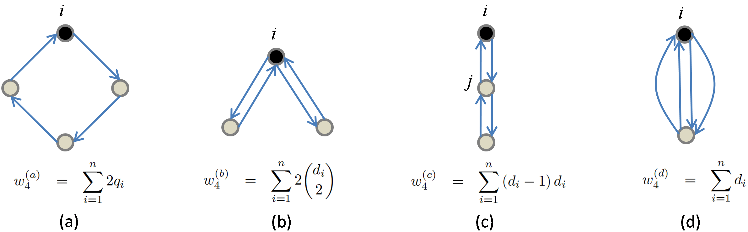
Figure 1: Enumeration of the possible types of closed walks of length $4$ in a graph with no self-loops. The classification is based on the structure of the subgraph underlying each closed walk. For each walk type, we also include an expression that corresponds to the number of closed walks of that particular type in terms of network structural properties.

A combinatorial analysis of (3) for $k=4$ gives us the following result:

Lemma III.3

Let $\mathcal{G}$ be a simple graph with adjacency matrix $A_{\mathcal{G}}$. Denote by $q_{i}$ and $d_{i}$ the number of quadrangles and edges touching node $i\in\mathcal{V}\left(\mathcal{G}\right)$, respectively. Then,

$$m_{4}\left(A_{\mathcal{G}}\right)=\frac{1}{n}\sum_{i\in\mathcal{V}\left(\mathcal{G}\right)}2q_{i}+4\binom{d_{i}}{2}+d_{i}.$$ (6)

Proof:

We compute the fourth moment from (3) by counting the number of closed walks of length 4 in $\mathcal{G}$. In Fig. 1, we enumerate all the possible types of closed walks of length $4$. We can count the number of closed walks of each particular type in terms of network structural features as follows:

(a)

The number of closed walks of type (a) is equal to twice the number of quadrangles, where the coefficient $2$ in $w_{4}^{\left(a\right)}$ accounts for the two possible directions (clockwise and counterclockwise) one can walk each quadrangle.

(b)

The number of walks of type (b) starting at node $i$ is equal to $2\binom{d_{i}}{2}$. The expression for $w_{4}^{\left(b\right)}$ comes from summing over all possible starting points, $i=1,...,n.$

(c)

The number of closed walks of this type can also be written in terms of the degrees as:

$$w_{4}^{\left(c\right)}=\sum_{i=1}^{n}\sum_{j=1}^{n}a_{ij}\left(d_{j}-1\right)=\sum_{j=1}^{n}\left(d_{j}-1\right)d_{j}.$$

(d)

The number of closed walks of this type starting at node $i$ is equal to $d_{i}$, thus, $w_{4}^{\left(d\right)}=\sum_{i=1}^{n}d_{i}$.

Hence, we obtain (6) by summing up all the above contributions, $w_{4}^{\left(a\right)}+w_{4}^{\left(b\right)}+w_{4}^{\left(c\right)}+w_{4}^{\left(d\right)}$, and simple algebraic manipulations). ∎

Lemma III.3 provides an expression to compute the fourth spectral moment in terms of structural features, namely, the distribution of degrees and quadrangles. We illustrate Lemma III.3 in the following example.

Example III.1

Consider the $n$-ring graph, $R_{n}$ (without self-loops). The eigenvalues of the adjacency matrix of the ring graph are $\lambda_{i}\left(A_{R_{n}}\right)=2\cos i\frac{2\pi}{n}$, for $i=0,1,...,n-1$. Hence, the fourth moment is equal to $m_{4}(A_{R_{n}})=\frac{1}{n}\sum_{i=0}^{n-2}\left(2\cos i\frac{2\pi}{n}\right)^{4}$, which (after some computations) can be found to be equal to $6$ for $n\not\in\left\{2,4\right\}$. We can reach this same result by directly applying (6), without performing an eigenvalue decomposition, as follows. In the ring graph, we have that $d_{i}=2$ and $q_{i}=0$, for $n\not\in\left\{2,4\right\}$. Hence, from (6), we directly obtain $m_{4}(A_{R_{n}})=6$, for $n\not\in\left\{2,4\right\}$.

The fourth spectral moment can be rewritten in terms of aggregated quantities, such as the total number of quadrangles and edges, and the sum-of-squares of the degrees, as follows:

Corollary III.4

Let $\mathcal{G}$ be a simple graph. Denote by $e$ and $Q$ the total number of edges and quadrangle in $\mathcal{G}$, respectively, and define $W_{2}=\sum_{i=1}^{n}d_{i}^{2}$. Then,

$$m_{4}\left(A_{\mathcal{G}}\right)=\frac{1}{n}\left[8Q+2W_{2}-2e\right].$$ (7)

Proof:

The proof comes straightforward from (6) by substituting $\sum_{i=1}^{n}q_{i}=4Q$ and $\sum_{i=1}^{n}d_{i}=2e.$ ∎

Hence, we do not need to have access to the detailed distribution of quadrangles and degrees in $\mathcal{G}$ to compute the fourth moment, we only need to know the aggregated quantities $Q$, $W_{2}$, and $e$.

III-C Fifth-Order Moment

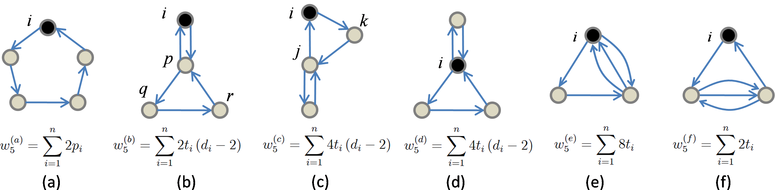
Figure 2: Possible types of closed walks of length $5$ in a simple graph. The classification is based on the structure of the subgraph underlying the closed walks. For each walk type, we also include an expression that corresponds to the number of closed walks of that particular type in terms of network structural features.

Lemma III.5

Let $\mathcal{G}$ be a simple graph. Denote by $p_{i}$, $t_{i}$, and $d_{i}$ the number of pentagons, triangles, and edges touching node $i\in\mathcal{V}\left(\mathcal{G}\right)$, respectively. Then,

$$m_{5}\left(A_{\mathcal{G}}\right)=\frac{1}{n}\sum_{i\in\mathcal{V}\left(\mathcal{G}\right)}2p_{i}+10t_{i}d_{i}-10t_{i}.$$ (8)

Proof:

The proof follows the same structure as that of Lemma III.3. A graphical representation of the types of closed walks of length 5 is provided in Fig. 2. Details regarding the counting of closed walks of each particular type can be found in the Appendix. ∎

Lemma III.5 expresses the fifth spectral moment of $A_{\mathcal{G}}$ in terms of network structural features. We can rewrite (8) in terms of aggregated quantities as follows:

Corollary III.6

Let $\mathcal{G}$ be a simple graph. Denote by $\Delta$ and $\Pi$ the total number of triangles and pentagons in $\mathcal{G}$, respectively. Define the degree-triangle correlation as $\mathcal{C}_{dt}=\sum_{i}d_{i}t_{i}$. Then,

$$m_{5}\left(A_{\mathcal{G}}\right)=\frac{1}{n}\left[10\Pi+10\mathcal{C}_{dt}-30\Delta\right].$$ (9)

Proof:

The proof comes from (8) taking into account that $\sum_{i=1}^{n}p_{i}=5\Pi$ and $\sum_{i=1}^{n}t_{i}=3\Delta.$ ∎

Observe how, as we increase the order of the moments, more complicated structural features appear in the expressions. In particular, the sum and sum-of-squares of the degrees influence the second and fourth spectral moments. (Notice that we can expand $\binom{d_{i}}{2}=\frac{1}{2}\left(d_{i}^{2}-d_{i}\right)$ in (6)). The total number of triangles in the network, $\Delta$, influences the third and fifth moments in (5) and (9). Also, the correlation between degree and triangle distributions, quantified by $\mathcal{C}_{dt}=\sum_{i}d_{i}t_{i}$, influences the fifth spectral moment in (9). We shall show in Section V that this structural correlation strongly influences the spectral radius of online social networks.

The main advantage of our results may not be apparent in networks with simple, regular structure. For these networks, an explicit eigenvalue decomposition is usually easy to compute and there may be no need to look for alternative ways to compute spectral properties. On the other hand, in the case of large-scale complex networks, the structure of the network can be very intricate —in many cases not even known exactly— and an explicit eigenvalue decomposition can be very challenging to compute, if not impossible. It is in these cases when the alternative approach proposed in this paper is most useful. In the following subsection, we use our expressions to compute the spectral moments of an online social network from empirical structural data.

III-D Spectral Moments of an Online Social Network

The real network under study is a subgraph of Facebook with $2,404$ nodes and $22,786$ edges obtained from crawling the graph in a breadth-first search around a particular node (the dataset can be found in [17]). Although the approach proposed in this section is meant to be used for much larger networks, we illustrate our results with this medium-size subgraph in order to compare our analysis with the results obtained from an explicit eigenvalue decomposition of the complete network topology.

In this example, we first compute the structural metrics involved in the first five spectral moments, in particular, the degree $d_{i}$, the number of triangles $t_{i}$, quadrangles $q_{i}$, and pentagons $p_{i}$ touching each node $i\in\mathcal{V}$. The degree $d_{i}$ and the number of triangles $t_{i}$ touching node $i$ can be easily computed by counting the number of edges attached to node $i$ and the number of edges connecting friends of $i$, respectively. In order to count the number of quadrangles $q_{i}$ and pentagons $p_{i}$ touching each node $i$, we must know the structure of the network around node $i$ with a radius of 2, i.e., node $i$ needs to know who her friends’ friends are. We denote by $\left|N_{i,2}\right|$ the number of nodes in the two-hops neighborhood around node $i$ (excluding node $i$). In order to count the number of quadrangles (resp. pentagons) touching node $i$, we must verify the presence of a cycle for each one of the $\binom{\left|N_{i,2}\right|}{3}$ (resp. $\binom{\left|N_{i,2}\right|}{4}$) subsets of three (resp. four) nodes in $N_{i,2}$.

In Fig. 3, we plot the distributions of degrees and triangles, as well as a scatter plot of $t_{i}$ versus $d_{i}$ (where each point has coordinates $\left(d_{i},t_{i}\right)$, in log-log scale, for all $i\in\mathcal{V}\left(\mathcal{G}\right)$). We then aggregate, via simple averaging, those structural metrics that are relevant to compute the spectral moments. In particular, we obtain the following numerical values for these metrics:

$$\begin{array}[]{ll}e/n=\sum d_{i}/2n=9.478,&\Delta/n=\sum t_{i}/3n=28.15,\\ Q/n=\sum q_{i}/4n=825.3,&\Pi/n=\sum p_{i}/5n=31,794,\\ W_{2}/n=\sum d_{i}^{2}/n=1,318,&\mathcal{C}_{dt}/n=\sum d_{i}t_{i}/n=8,520.\end{array}$$

Hence, using these values in expressions (4), (7), and (9), we obtain the following spectral moments: $m_{1}\left(A_{\mathcal{G}}\right)=0,$ $m_{2}\left(A_{\mathcal{G}}\right)=18.95,$ $m_{3}\left(A_{\mathcal{G}}\right)=168.9,$ $m_{4}\left(A_{\mathcal{G}}\right)=9,230,$ and $m_{5}\left(A_{\mathcal{G}}\right)=402,310.$

In this section, we have derived expressions to compute the first five spectral moment of $A_{\mathcal{G}}$ from network structural properties. In the next section, we use semidefinite programming to extract bounds on spectral properties of interest from a sequence of spectral moments.

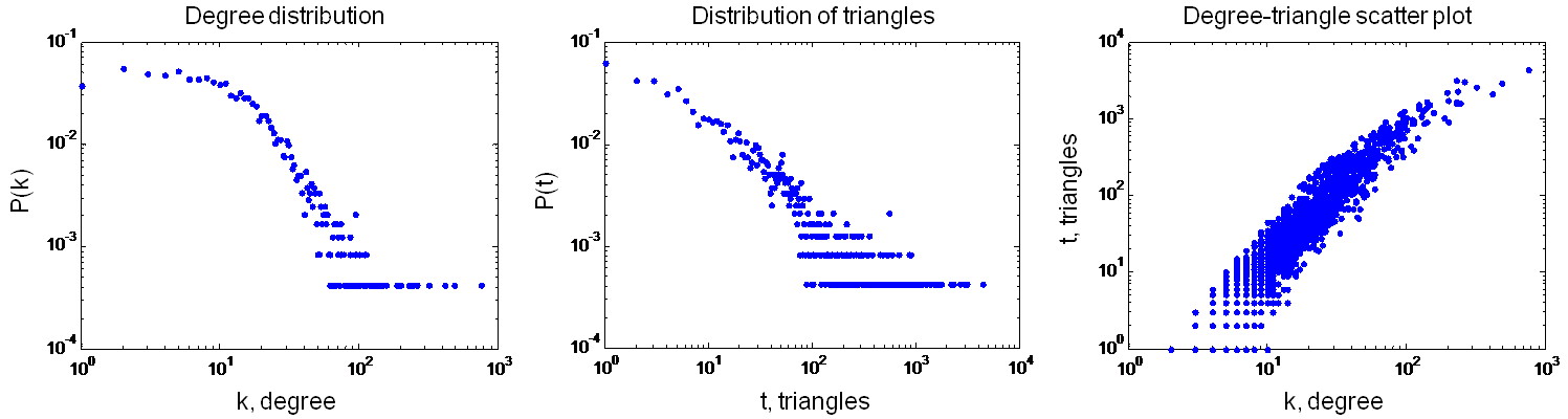
Figure 3: In the left and center figures, we plot the distributions of degrees and triangles of the social network under study (in log-log scale). In the right figure, we include a scatter plot where each point has coordinates $(d_{i},t_{i})$, in log-log scale, for all the nodes in the social graph.

IV Optimal Spectral Bounds from Spectral Moments

In this section, we introduce an approach to derive bounds on a network spectral properties from its sequence of spectral moments. Since we have expressions for the spectral moments in terms of structural properties, these bounds relate the eigenvalues of a network with its structural properties. For this purpose, we adapt an optimization framework proposed in [18] and [19] to derive optimal probabilistic bounds on a random variable from a sequence of moments of its probability distribution. In order to use this framework, we first need to introduce a probabilistic interpretation of a network eigenvalue spectrum and its spectral moments.

For a simple graph $\mathcal{G}$, we define its spectral density as,

$$\mu_{\mathcal{G}}\left(x\right)=\frac{1}{n}\sum_{i=1}^{n}\delta\left(x-\lambda_{i}\right),$$ (10)

where $\delta\left(\cdot\right)$ is the Dirac delta function and $\left\{\lambda_{i}\right\}_{i=1}^{n}$ is the set of (real) eigenvalues of the symmetric adjacency matrix $A_{\mathcal{G}}$. Let us define a random variable $X$ with probability density $\mu_{\mathcal{G}}$. The moments of $X\sim\mu_{\mathcal{G}}$ are equal to the spectral moments of $A_{\mathcal{G}}$, i.e.,

$$\mathbb{E}_{\mu_{\mathcal{G}}}\left(X^{k}\right) =\int_{\mathbb{R}}x^{k}\mu_{\mathcal{G}}\left(x\right)dx$$

$$=\frac{1}{n}\sum_{i=1}^{n}\int_{\mathbb{R}}x^{k}\delta\left(x-\lambda_{i}\right)dx$$

$$=\frac{1}{n}\sum_{i=1}^{n}\lambda_{i}^{k}=m_{k}\left(A_{\mathcal{G}}\right),$$

for all $k\geq 0$. Furthermore, for a given Borel measurable set $T$, we have

$$\Pr\left(X\in T\right)=\int_{x\in T}\mu_{\mathcal{G}}\left(x\right)dx=\frac{1}{n}\left|\left\{\lambda_{i}:\lambda_{i}\in T\right\}\right|.$$

In other words, the probability of the random variable $X$ being in a set $T$ is proportional to the number of eigenvalues of $A_{\mathcal{G}}$ in $T$.

In this probabilistic context, we can study two problems that are relevant for the network dynamical behavior. Given a truncated sequence of spectral moments, we formulate these problems as follows:

Problem 1

Find optimal bounds on the number of eigenvalues that can lie in a given interval $T$.

Problem 2

Find bounds on the smallest and largest eigenvalues of $A_{\mathcal{G}}$.

In the following subsections, we provide solutions to each one of the above problems, from only the knowledge of a truncated sequence of moments.

IV-A Solution to Problem 1

Our solution is based on the following classical problem in analysis:

Problem 3 (Moment Problem)

Given a sequence of moments $\left(m_{0},...,m_{k}\right)$, and Borel measurable sets $T\subseteq\Omega\subseteq\mathbb{R}$, compute:

$$\begin{array}[]{lrll}Z_{P}=&\max_{\mu}&\int_{T}1\,d\mu&\\ &\text{s.t.}&\int_{\Omega}x^{j}\,d\mu=m_{j},&\text{for }j=0,1,...,k.\end{array}$$ (11)

where $\mu\in\mathbb{M}\left(\Omega\right)$, $\mathbb{M}\left(\Omega\right)$ being the set of positive Borel measures supported by $\Omega$.

The solution to this problem provides an extension to the classical Markov and Chebyshev’s inequalities in probability theory when moments of order greater than 2 are available. In [18] and [19], it was shown that the optimal value of $Z_{P}$ can be efficiently computed by solving a single semidefinite program using a dual formulation. Before we introduce this dual formulation, it is important to discuss some details regarding the feasibility of this problem.

A sequence of moments $\mathbf{m}_{k}=\left(m_{0},m_{1},...,m_{k}\right)$ is said to be feasible in $\Omega$ if there exists a measure $\mu\in\mathbb{M}\left(\Omega\right)$ whose moments match those in the sequence $\mathbf{m}_{k}$. In general, an arbitrary sequence of numbers may not correspond to a feasible sequence of moments. The problem of deciding whether or not a sequence of numbers is a feasible sequence of moments is called the classical moment problem [20]. Depending on the set $\Omega$, we find three important instances of this problem:

(i) the Hamburguer moment problem, when $\Omega=\mathbb{R}$,

(ii) the Stieltjes moment problem, when $\Omega=\mathbb{R}_{+}$, and

(iii) the Hausdorff moment problem, when $\Omega=\left[0,1\right]$.

For univariate distributions, necessary and sufficient conditions for feasibility of these instances of the classical moment problem can be given in terms of certain matrices being positive semidefinite, as follows. Let us define, for any $s\geq 0$, the following Hankel matrices of moments,

$$R_{2s} =\left[\begin{array}[]{cccc}m_{0}&m_{1}&\cdots&m_{s}\\ m_{1}&m_{2}&\cdots&m_{s+1}\\ \vdots&\vdots&\ddots&\vdots\\ m_{s}&m_{s+1}&\cdots&m_{2s}\end{array}\right],$$ (16)

$$R_{2s+1} =\left[\begin{array}[]{cccc}m_{1}&m_{2}&\cdots&m_{s+1}\\ m_{2}&m_{3}&\cdots&m_{s+2}\\ \vdots&\vdots&\ddots&\vdots\\ m_{s+1}&m_{s+2}&\cdots&m_{2s+1}\end{array}\right].$$ (21)

Then, we have the following feasibility results for the Hamburguer moment problem [20]:

Theorem IV.1

A necessary and sufficient condition for a sequence of moments $\mathbf{m}_{k}=\left(m_{0},m_{1},...,m_{2s}\right)$ to be feasible in $\Omega=\mathbb{R}$ is $R_{2s}\succeq 0$.

Notice that the Hankel matrix associated to the sequence of spectral moments $\left(1,m_{1}\left(A_{\mathcal{G}}\right),...,m_{2s}\left(A_{\mathcal{G}}\right)\right)$ of a finite graph $\mathcal{G}$ always satisfy Hamburguer feasibility condition, $R_{2s}\succeq 0$. We now describe the dual formulation proposed in [18] and [19] to compute the solution of the infinite-dimensional optimization problem in (11) by solving a single semidefinite program.

Using duality theory, one can associate a dual variable $y_{i}$ to each equality constraint of the primal (11) to obtain (see [19] for more details):

$$\begin{array}[]{lrll}Z_{D}=&\min_{y_{i}}&\sum_{i=0}^{k}y_{i}m_{i}&\\ &\text{s.t.}&\sum_{i=0}^{k}y_{i}x^{i}-1\geq 0\text{,}&\text{for }x\in T,\\ &&\sum_{i=0}^{k}y_{i}x^{i}\geq 0\text{,}&\text{for }x\in\Omega.\end{array}$$ (22)

Notice that the dual constrains are univariate polynomials in $x$. Since a univariate polynomial is nonnegative if and only if it can be written as sum of squares of polynomials, the dual problem can be formulated as a sum-of-squares program (SOSP) that can be numerically solved via semidefinite programming. (For more details on SOSP and SDP, the interested reader is referred to [21] and [22].) Karlin and Isii proved the following result concerning strong duality [23]:

Theorem IV.2

If the Hankel matrix of moments $R_{2s}$ defined in (16) is positive definite, then $Z_{P}=Z_{D}$.

From Theorem IV.1, we have that a sequence of spectral moments satisfy strong duality if $\det R_{2s}\neq 0$. This determinant is zero only for very degenerate networks, and we assume strong duality holds for the networks studied in this paper.

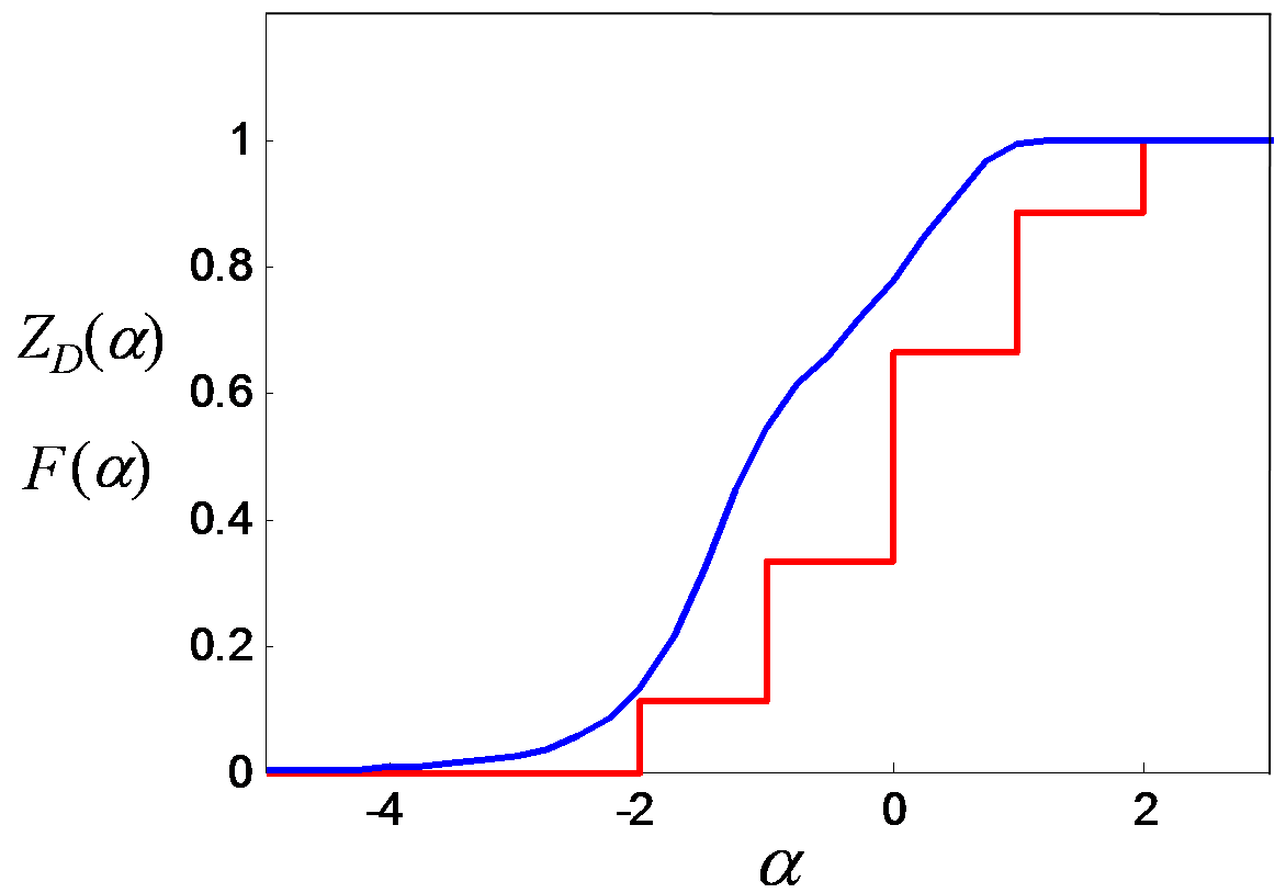
Figure 4: Numerical solution of the SOSP described in Example IV.1. The stairs-like function corresponds to the cumulative density function of $\mu_{\mathcal{G}}$, $F(\alpha)$. Observe how the (numerical) function $Z_{D}\left(\alpha\right)$ is greater (or equal) to $F(\alpha)$ for all values of $\alpha$.

The optimization framework we have described above can be used to solve Problem 1, since the solution of the dual problem in (22), when $m_{j}=m_{j}\left(A_{\mathcal{G}}\right)$ for $j=1,2,...,k$, satisfies:

$$Z_{D}\geq\int_{T}1~{}d\mu_{\mathcal{G}}=\frac{1}{n}\left|\left\{\lambda_{i}:\lambda_{i}\in T\right\}\right|,$$ (23)

where $\mu_{\mathcal{G}}$ is the spectral density of $\mathcal{G}$. Then, $Z_{D}$ is the optimal upper bound on the number of eigenvalues of $A_{\mathcal{G}}$ that lie in the set $T$ given a truncated sequence of spectral moments. We illustrate this result in the following example.

Example IV.1

Let us consider the spectral distribution $\mu_{\mathcal{G}}=\frac{1}{n}\sum_{i}w_{i}\delta\left(x-x_{i}\right)$, with atomic masses located at $\left(x_{i}\right)_{1\leq i\leq 5}=\left(-2,-1,0,1,2\right)$ and weights $\left(w_{i}\right)_{1\leq i\leq 5}=\left(1/9,2/9,3/9,2/9,1/9\right)$. The sequence of moments of $\mu_{\mathcal{G}}$ is $\left(m_{k}\right)_{1\leq i\leq 5}=\left(0,4/3,0,4,0\right)$. Let us define $F\left(\alpha\right)\triangleq\int_{-\infty}^{\alpha}\mu_{\mathcal{G}}\left(x\right)dx$, i.e., the cumulative distribution of $\mu_{\mathcal{G}}\left(x\right)$, and denote by $Z_{D}\left(\alpha\right)$ the numerical solution to the dual SOSP in (22) for $T=\left(-\infty,\alpha\right]$. According to (23), $Z_{D}\left(\alpha\right)$ is an upper bound of $F\left(\alpha\right)$ for all values of $\alpha$. In Fig. 4, we verify this result by plotting the cumulative distribution $F\left(\alpha\right)$ and $Z_{D}\left(\alpha\right)$ for $\alpha=\left[-5:0.25:3\right]$.

IV-B Solution to Problem 2

In this subsection, we derive bounds on the smallest and largest eigenvalues of $A_{\mathcal{G}}$ from only the knowledge of a truncated sequence of spectral moments. For this purpose, we apply the technique proposed in [24] to compute the smallest interval $\left[a,b\right]$ containing the support of a positive Borel measure $\mu$ from its complete sequence of moments $\left(m_{r}\right)_{r\geq 0}$. In [24] a technique was also proposed to compute tight bounds on the values of $a$ and $b$ when only a truncated sequence of moments $\left(m_{r}\right)_{0\leq r\leq k}$ is known. In the context of spectral graph theory, we can apply this technique to a sequence of spectral moments in order to bound the support of the spectral measure $\mu_{\mathcal{G}}$ of a graph $\mathcal{G}$. In this context, the extreme values, $a$ and $b$, of the smallest interval containing the support of $\mu_{\mathcal{G}}$ corresponds to the minimum and maximum eigenvalues of $A_{\mathcal{G}}$, denoted by $\lambda_{\min}\left(A_{\mathcal{G}}\right)$ and $\rho\left(A_{\mathcal{G}}\right)$, respectively. Since we can compute the first five spectral moments in terms of structural properties using the results in Section III, this technique allows to compute bounds on $\lambda_{\min}\left(A_{\mathcal{G}}\right)$ and $\rho\left(A_{\mathcal{G}}\right)$ in terms of structural properties.

We describe the scheme proposed in [24] to compute the smallest interval $\left[a,b\right]$ by solving a series of SDPs in one variable. As we shall show below, at step $s$ of this series of SDPs, we are given a sequence of moments $\left(m_{1},...,m_{2s+1}\right)$ and solve two SDPs whose solution provides an inner approximation $\left[\alpha_{s},\beta_{s}\right]\subseteq\left[a,b\right]$. As we increase $s$ in this series, we obtain two sequences $\left(\alpha_{s}\right)_{s\in\mathbb{N}}$ and $\left(\beta_{s}\right)_{s\in\mathbb{N}}$ that are respectively monotone nonincreasing and nondecreasing, and converge to $a$ and $b$ as $s\rightarrow\infty$. In our case, we have expressions for the first five spectral moments, $\left(m_{1},...,m_{5}\right)$, hence, we can solve the first two steps of the series of SDPs. The solutions, $\alpha_{s}$ and $\beta_{s}$, of these SDPs provide upper and lower bounds on $\lambda_{\min}\left(A_{\mathcal{G}}\right)$ and $\rho\left(A_{\mathcal{G}}\right)$, respectively, in terms of structural properties.

In order to formulate the series of SDPs proposed in [24] we need to define the so-called localizing matrix [25]. Given a sequence of moments, $\mathbf{m}^{\left(2s+1\right)}=\left(m_{1},...,m_{2s+1}\right)$, the localizing matrix is a Hankel matrix defined as:

$$H_{s}\left(c\right)\triangleq R_{2s+1}-c~{}R_{2s}\text{,}$$ (24)

where $R_{2s}$ and $R_{2s+1}$ are the Hankel matrices of moments defined in (16). Hence, for a given sequence of moments, the entries of $H_{s}\left(c\right)$ depend affinely on the variable $c$. Then, we can compute $\alpha_{s}$ and $\beta_{s}$ as follows [24]:

Proposition 1

Let $\mathbf{m}^{\left(2s+1\right)}=\left(m_{1},...,m_{2s+1}\right)$ be the truncated sequence of moments of a positive Borel measure $\mu$. Then,

$$a \leq\alpha_{s}\triangleq\max_{\alpha}\left\{\alpha:H_{s}\left(\alpha\right)\succcurlyeq 0\right\},$$ (25)

$$b \geq\beta_{s}\triangleq\min_{\beta}\left\{\beta:-H_{s}\left(\beta\right)\succcurlyeq 0\right\},$$ (26)

for $\left[a,b\right]$ being the smallest interval containing $supp(\mu)$.

Remark IV.1

Observe that $\alpha_{s}$ and $\beta_{s}$ are the solutions to two SDPs in one variable, which can be efficiently solved using standard optimization software (for example, CVX [26]). Notice that the matrix involved in the semidefinite constrains in (25) and (26), $H_{s}\left(x\right)$, has size $(s+1)\times(s+1)$. Hence, the computational complexity of solving this SDP is polynomial in $s$, [24]. Since $s$ is a small number in our context (i.e., $s=2$ if we use five moments in Proposition 1), the computational cost of solving this SDP is negligible in comparison with the cost of counting triangles, quadrangles and pentagons in $\mathcal{G}$, which requires $\sum_{i=1}^{n}\binom{N_{i,1}}{2}$, $\sum_{i=1}^{n}\binom{N_{i,2}}{3}$, and $\sum_{i=1}^{n}\binom{N_{i,2}}{4}$ operations, respectively.

Given a truncated sequence of spectral moments, the smallest interval $\left[a,b\right]$ becomes $\left[\lambda_{\min}\left(A_{\mathcal{G}}\right),\rho\left(A_{\mathcal{G}}\right)\right]$, thus, Proposition 1 provide an efficient numerical scheme to compute the bounds $\alpha_{s}\geq\lambda_{\min}\left(A_{\mathcal{G}}\right)$ and $\beta_{s}\leq\rho\left(A_{\mathcal{G}}\right)$. Furthermore, for $s=1$ and $2$, one can analytically solve the SDPs in (25) and (26). For example, in the case $s=1$, we are given a sequence of three spectral moments, $\left(m_{1},m_{2},m_{3}\right)$, with localizing matrix

$$H_{1}\left(c\right)=\left[\begin{array}[]{cc}m_{1}-cm_{0}&m_{2}-cm_{1}\\ m_{2}-cm_{1}&m_{3}-cm_{2}\end{array}\right].$$

From (5), the spectral moments of simple graphs satisfy $m_{0}=1$, $m_{1}=0$, $m_{2}=2e/n$, and $m_{3}=6\Delta/n$. One can prove that the optimal values of $\alpha_{1}$ and $\beta_{1}$ are the smallest and largest root of $\det H_{1}(c)=0$, which is a second-order polynomial in the variable $c$. Then, we have the following bounds on $\rho\left(A_{\mathcal{G}}\right)$ and $\lambda_{\min}\left(A_{\mathcal{G}}\right)$ in terms of the number of nodes $n$, edges $e$, and triangles $\Delta$ in $\mathcal{G}$:

$$\rho\left(A_{\mathcal{G}}\right) \geq\beta_{1}=\frac{6\Delta+\sqrt{36\Delta^{2}+32e^{3}/n}}{4e},$$ (27)

$$\lambda_{\min}\left(A_{\mathcal{G}}\right) \leq\alpha_{1}=\frac{6\Delta-\sqrt{36\Delta^{2}+32e^{3}/n}}{4e}.$$

As mentioned above, tighter bounds on the spectral radius can be found as we increase the value of $s$ in Proposition 1. In the case $s=2$, we are given a sequence of five spectral moments $\left(m_{1},m_{2},...,m_{5}\right)$ with localizing matrix,

$$H_{2}\left(c\right)=\left[\begin{array}[]{ccc}m_{1}-c&m_{2}-cm_{1}&m_{3}-cm_{2}\\ m_{2}-cm_{1}&m_{3}-cm_{2}&m_{4}-cm_{3}\\ m_{3}-cm_{2}&m_{4}-cm_{3}&m_{5}-cm_{4}\end{array}\right].$$ (28)

As we proved in Section III, these moments depend on the number of nodes, edges, cycles of length 3 to 5, the sum of squares of degrees $W_{2}$, and the degree-triangle correlation $\mathcal{C}_{dt}$. Since we are using much richer structural information than in the case $s=1$, we should expect the resulting bounds to be substantially tighter (as we shall verify in Section V). For $s=2$, the optimal values $\alpha_{2}$ and $\beta_{2}$ can also be analytically computed, as follows. First, note that $-H_{2}(c)\succcurlyeq 0$ if and only if all the eigenvalues of $H_{2}$ are nonpositive. The characteristic polynomial of $H_{2}\left(c\right)$ can be written as

$$\phi_{2}\left(\lambda\right)\triangleq\det\left(\lambda I-H_{2}(c)\right)=\lambda^{3}+p_{1}\lambda^{2}+p_{2}\lambda+p_{3},$$

where $p_{j}$ is a polynomial of degree $j$ in the variable $c$ (with coefficients depending on the moments). Thus, by Descartes’ rule, all the eigenvalues of $H_{2}$ are nonpositive if and only if $p_{j}\geq 0$, for $j=1,2,$ and $3$. In fact, one can prove that the optimal values of $\alpha_{2}$ and $\beta_{2}$ in (25) and (26) can be computed as the smallest and largest roots of $p_{3}\left(c\right)=\det H_{2}\left(c\right)=0$, which is a third degree polynomial in the variable $c$ [24]. Therefore, the expressions that allow us to compute the optimal bounds are:

$$\rho\left(A_{\mathcal{G}}\right) \geq\beta_{2}=\max\{\text{roots}[p_{3}(c)]\},$$ (29)

$$\lambda_{\min}\left(A_{\mathcal{G}}\right) \leq\alpha_{2}=\min\{\text{roots}[p_{3}(c)]\},$$

where $p_{3}\left(c\right)=d_{3}c^{3}+d_{2}c^{2}+d_{1}c+d_{0,}$ with

$$d_{0} \triangleq 2m_{2}m_{3}m_{4}-m_{5}m_{2}^{2}-m_{3}^{3}+m_{1}m_{5}m_{3}-m_{1}m_{4}^{2},$$

$$d_{1} \triangleq m_{2}m_{3}^{2}-m_{2}^{2}m_{4}+m_{1}m_{5}m_{2}-m_{1}m_{3}m_{4}$$

$$-m_{5}m_{3}+m_{4}^{2},$$

$$d_{2} \triangleq m_{4}m_{1}m_{2}-m_{5}m_{1}^{2}+m_{1}m_{3}^{2}-m_{2}^{2}m_{3}$$

$$+m_{5}m_{2}-m_{4}m_{3},$$

$$d_{3} \triangleq m_{4}m_{1}^{2}-2m_{1}m_{2}m_{3}+m_{2}^{3}-m_{4}m_{2}+m_{3}^{2}.$$

There are closed-form expressions for the roots of this third-order polynomial (for example, Cardano’s formula [27]), although the resulting expressions for the roots are rather complicated and do not provide much insight.

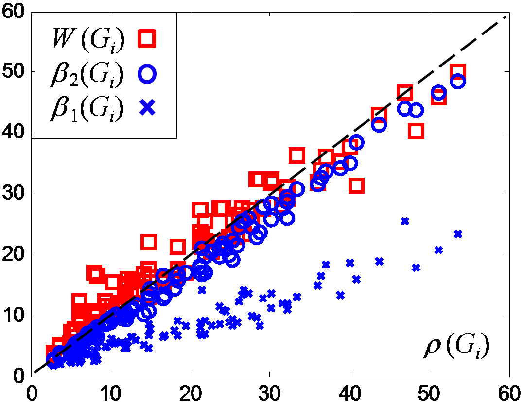
Figure 5: Scatter plot of the spectral radius, $\rho\left(G_{i}\right)$, versus the lower bounds $\beta_{1}\left(G_{i}\right)$ (crosses) and $\beta_{2}\left(G_{i}\right)$ (circles), as well as the random–graph-based estimator $W\left(G_{i}\right)$ (squares), where each point is associated with one of the $100$ social subgraphs considered in our experiments.

In this subsection, we have presented a convex optimization framework to compute optimal bounds on the maximum and minimum eigenvalues of a graph $\mathcal{G}$ from a truncated sequence of its spectral moments. Since we have expressions for spectral moments in terms of structural properties, these bounds relate the eigenvalues of a graph with its structural properties.

V Numerical Simulations and Structural Implications

In this section, we analyze real data from a regional network of Facebook that spans $63,731$ users (nodes) connected by $817,090$ friendships (edges) [28]. In order to corroborate our results in different network topologies, we extract multiple medium-size social subgraphs from the Facebook graph by running a Breath-First Search (BFS) around different starting nodes. Each BFS induces a social subgraph spanning all nodes 2 hops away from a starting node. We use this approach to generate a set $\mathbf{G}=\{G_{i}\}_{i\leq 100}$ of 100 different social subgraphs centered around 100 randomly chosen nodes.

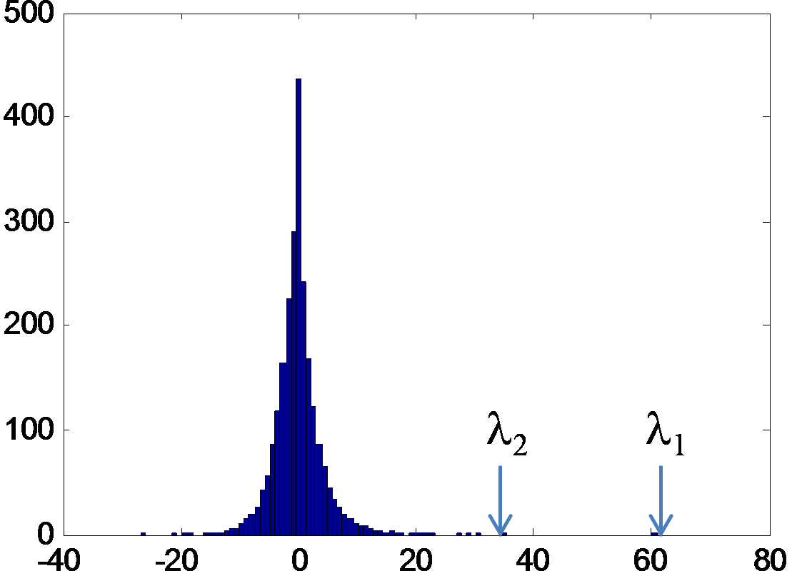
Figure 6: Histogram of eigenvalues of a social subgraph of Facebook with 2,404 nodes.

In our first numerical experiment, we compute the first five spectral moments $\mathbf{m}_{5}\left(G_{i}\right)=\left(m_{1}\left(G_{i}\right),...,m_{5}\left(G_{i}\right)\right)$ for each social subgraph $G_{i}\in\mathbf{G}$. From these moments, we then compute the lower bounds on the spectral radius $\beta_{1}\left(G_{i}\right)$ and $\beta_{2}\left(G_{i}\right)$ using Proposition 1. Fig. 5 is a scatter plot where each cross has coordinates $\left(\rho\left(G_{i}\right),\beta_{1}\left(G_{i}\right)\right)$ and each circle has coordinates $\left(\rho\left(G_{i}\right),\beta_{2}\left(G_{i}\right)\right)$, for all $G_{i}\in\mathbf{G}$. In the same figure, we have also included a cloud of red squares with coordinates $\left(\rho\left(G_{i}\right),W\left(G_{i}\right)\right)$, where $W\left(G_{i}\right)\triangleq\left.\sum_{i}d_{i}^{2}\right/\sum_{i}d_{i}$ is the estimator based on synthetic random graphs (2). Observe how the spectral radii $\rho\left(G_{i}\right)$ of these social subgraphs are remarkably close to the theoretical lower bound $\beta_{2}\left(G_{i}\right)$. In particular, the correlation coefficient between $\rho\left(G_{i}\right)$ and $\beta_{2}\left(G_{i}\right)$ is equal to 0.995 (while the correlation between $\rho\left(G_{i}\right)$ and the estimator based on random networks, $W\left(G_{i}\right)$, is equal to 0.974). Therefore, it is reasonable to use $\beta_{2}\left(G_{i}\right)$ as an estimate of $\rho\left(G_{i}\right)$ for social subgraphs.

In what follows, we analyze the spectral moments of online social networks to reveal the set of structural properties having the highest impact on the spectral radius. Empirical evidence strongly suggests that many real-world networks present heavy-tailed eigenvalue distributions [29],[30]. For example, in Fig. 6 we have included the histogram of eigenvalues of a subgraph of Facebook with $2,404$ nodes, where we can observe the following two typical properties in the spectrum of online social networks: ($i$) The largest eigenvalue of the network is well separated from the rest of eigenvalues (spectral dominance), and ($ii$) the bulk of eigenvalues concentrates around the origin. In this case, we can numerically approximate high-order moments as $m_{k}\left(A_{\mathcal{G}}\right)\approx\frac{1}{n}\lambda_{1}^{k}$. Furthermore, we have from (9) that the fifth spectral moment is equal to $m_{5}\left(A_{\mathcal{G}}\right)=\frac{1}{n}\left[10\Pi+10\mathcal{C}_{dt}-30\Delta\right]\approx\frac{1}{n}\lambda_{1}^{5}$. Therefore, we have the following estimator for the spectral radius of online social networks:

$$\lambda_{1}\approx\tilde{\lambda}_{1}^{\left(a\right)}\triangleq\left(10\Pi+10\mathcal{C}_{dt}-30\Delta\right)^{1/5}\text{.}$$ (30)

For example, for the social subgraph with 2,404 nodes mentioned above, the exact value of the spectral radius is $\lambda_{1}=60.9$, while the estimator is $\tilde{\lambda}_{1}^{(a)}=62.6$.

We now use (30) to unveil the set of structural properties that are most influential on the spectral radius. In Fig. 7, we plot (in semilog scale) the values of $\Pi$, $\mathcal{C}_{dt}$, and $\Delta$ for each one of the 100 different social subgraphs, $G_{i}\in\mathbf{G}$, considered in our previous experiment. Observe how the number of triangles $\Delta$ is always much smaller than $\Pi+\mathcal{C}_{dt}$. Therefore, for online social networks, we can simplify (30) as follows,

$$\lambda_{1}\approx\tilde{\lambda}_{1}^{\left(b\right)}\triangleq\left(10\Pi+10\mathcal{C}_{dt}\right)^{1/5}.$$

Fig. 8 is a scatter plot where each circle has coordinates $(\rho\left(G_{i}\right),\tilde{\lambda}_{1}^{\left(b\right)}\left(G_{i}\right))$, for all $G_{i}\in\mathbf{G}$. We observe how our approximation presents an excellent performance in practice, outperforming the popular estimator, $W\left(G_{i}\right)$, based on random networks (see Fig. 5).

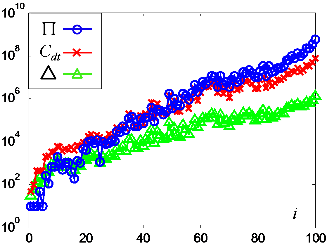
Figure 7: Number of triangles $\Delta$ (green triangles), degree-triangle correlation $C_{dt}$ (red crosses), and number of pentagons $\Pi$ (blue circles) for each one of the $100$ social subgraphs considered in our experiments (in semilog scale).

The estimator $\tilde{\lambda}_{1}^{\left(b\right)}$ provides a clear insight about what structural properties have the strongest impact in the spectral radius of online social networks. In particular, $\tilde{\lambda}_{1}^{\left(b\right)}$ unveils that both the number of pentagons, $\Pi$, and the degree-triangle correlation, $\mathcal{C}_{dt}$, are structural properties with a strong influence on the spectral radius.

The tightness of our bounds depends on the nature of the data used. In the following examples, we illustrate the quality of our bounds for an Internet and an e-mail network:

Example V.1 (Enron e-mail network)

In this example we study the spectral properties of a subgraph of the Enron e-mail network [32]. In this network, nodes correspond to e-mail addresses and an edge $\left(i,j\right)$ exists if $i$ sent at least one e-mail to $j$ (or vice versa). The subgraph under study has $n=3,215$ nodes, $e=36,537$ edges, and its largest eigenvalue is $\lambda_{1}=95.18$. Using the results in Section III, we compute the first five spectral moments of the adjacency matrix to be: $m_{1}=0$, $m_{2}=22.47$, $m_{3}=394.7$, $m_{4}=33,491$, and $m_{5}=2,603,200$. From Proposition 1, we obtain the following lower bound on the largest eigenvalue: $\beta_{2}=78.53<\lambda_{1}$. We can also compare our bound with the estimator in (2), corresponding to a random network with the same degree distribution. The value of the estimator is equal to $\tilde{\lambda}_{1}=124.57$.

Example V.2 (AS-Skitter Internet network)

We now consider a subgraph of the Internet network at the Autonomous Systems (AS) level, which was obtained from the Skitter data collection in CAIDA [33]. Our subgraph has $n=2,248$ nodes, $e=20,648$ edges, and its largest eigenvalue at $\lambda_{1}=91.3$. The spectral moments of its adjacency matrix are $m_{1}=0$, $m_{2}=18.37$, $m_{3}=341.1$, $m_{4}=40,001$, and $m_{5}=2,777,018$, and the resulting lower bound is $\beta_{2}=74.72<\lambda_{1}$. In this case, the estimator based on random networks produces a value of $\tilde{\lambda}_{1}=219.1$, which is very loose. Therefore, estimators based on random networks can be very misleading in the analysis of the Internet graph.

In this section, we have first shown that $\beta_{2}\left(G_{i}\right)$ can be used as an estimator of the spectral radius $\rho\left(G_{i}\right)$ for online social subgraphs, outperforming the estimator based on random networks. Furthermore, we have analyzed the spectral moments of online social networks to unveil the set of structural properties having the highest impact on the spectral radius. In particular, we have found that the number of pentagons and the degree-triangle correlation strongly influence the spectral radius of online social networks.

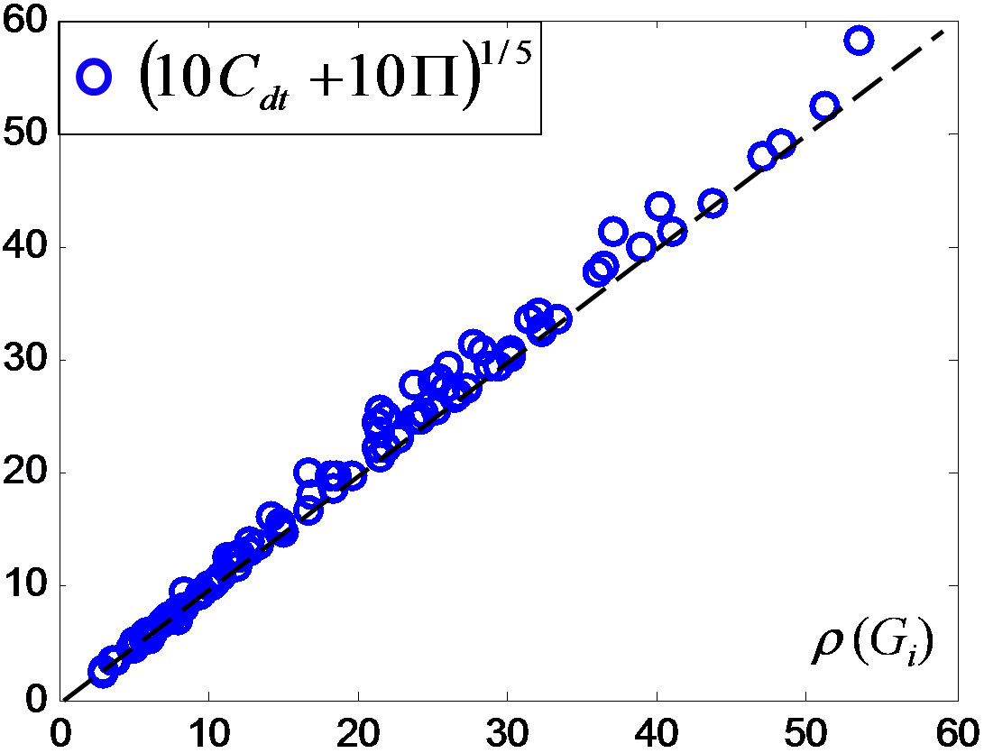
Figure 8: Scatter plot of the spectral radius, $\rho\left(G_{i}\right)$, versus the spectral estimator $\tilde{\lambda}_{i}^{\left(b\right)}\left(G_{i}\right)$, where each circle is associated with one of the $100$ social subgraphs considered in our experiments.

VI Conclusions

A fundamental question in the field of network science is to understand the relationship between the structural properties of a network and its dynamical performance. The common approach to study this relationship is to use synthetic network models. Although very common, synthetic models present some major flaws: (i) These models are only suitable to study a very limited range of structural properties, and (ii) they implicitly induce structural properties that are not directly controlled and can influence the network dynamical performance.

In this paper, we have proposed an alternative approach to study the relationship between a network structure and its dynamics that is not based on synthetic models. Our approach exploits the closed connection between the dynamical performance of many dynamical processes that can take place in a network and its eigenvalue spectrum. Consequently, we have studied how structural properties of a network relate to its eigenvalue spectrum using algebraic graph theory and convex optimization. In particular, we have derived expressions that explicitly relate structural properties of a network with its spectral moments. We have also introduced an optimization framework that allows us to extract optimal bounds on spectral properties of interest using semidefinite programming.

Using our approach, we have unveiled those structural properties that have the strongest impact on the spectral properties of a collection of social subgraphs. In particular, we have found that the number of close cycles of lengths 3 to 5 (quantified by $\Delta$, $Q$ and $\Pi$), as well as the sum and sum-of-squares of the degrees, and the degree-triangle correlation $\mathcal{C}_{dt}$ have a direct influence on the eigenvalue spectrum. Furthermore, in the case of online social networks, we have found that the number of pentagons and the degree-triangle correlation strongly influence the spectral radius of the network.

Appendix A Proof of Lemma III.5

Lemma III.5 Let $\mathcal{G}$ be a simple graph. Denote by $p_{i}$, $t_{i}$, and $d_{i}$ the number of pentagons, triangles, and edges touching node $i$ in $\mathcal{G}$, respectively. Then,

$$m_{5}\left(A_{\mathcal{G}}\right)=\frac{1}{n}\left[\sum_{i=1}^{n}2p_{i}+10t_{i}d_{i}-10t_{i}\right].$$

Proof:

As in Lemma III.3, we count the number of closed walks of length $5$ in $\mathcal{G}$. We classify these walks based on the structure of the subgraph underlying each walk. We provide a classification of the walk types in Fig. 2, where we also include expressions for the number of closed walks of each type. We now provide the details on how to compute those expressions for each walk type:

(a)

The number of closed walks of this type starting at $i$ is equal to twice the number of pentagons touching $i$, hence, the total number is given by $\sum_{i=1}^{n}2p_{i}$.

(b)

In order to count walks of this type, it is convenient to define $t_{pqr}$ as the indicator function that takes value $1$ if there exists a triangle connecting vertices $p$, $q$, and $r$ (0, otherwise). Note that this indicator satisfies $\sum_{q=1}^{n}\sum_{r=1}^{n}t_{pqr}=2t_{p}$, where $t_{p}$ is the number of triangles touching node $p$. Hence, the number of closed walks of type (b) can be written as:

$$w_{5}^{\left(b\right)}=\sum_{i=1}^{n}\sum_{p=1}^{n}\sum_{q\neq i}\sum_{r\neq i}a_{ip}t_{pqr},$$

where $a_{ip}$ indicates the existence of an edge from $i$ to $p$, and $t_{pqr}$ indicates the existence of a triangle connecting $q$ and $r$ with $p$. We can then perform the following algebraic manipulations,

$$w_{5}^{\left(b\right)} \overset{(i)}{=}\sum_{p=1}^{n}\sum_{q=1}^{n}\sum_{r=1}^{n}t_{pqr}\left(\sum_{i\neq q,r}a_{ip}\right)$$

$$\overset{(ii)}{=}\sum_{p=1}^{n}\left(d_{p}-2\right)\sum_{q=1}^{n}\sum_{r=1}^{n}t_{pqr}$$

$$=2\sum_{p=1}^{n}t_{p}\left(d_{p}-2\right),$$

where in equality ($i$) we have changed the order of the subindices, and impose the inequality constrains on subindex $i$. In equality ($ii$), we take into account that $\sum_{i\neq q,r}a_{ip}=d_{i}-2$, since $p$ is connected to $q$ and $r$ in this walk type.

(c)

We can use the indicator function $t_{ijk}$ to write the total number of walks in this type as follows,

$$w_{5}^{\left(c\right)} =2\sum_{i=1}^{n}\sum_{j=1}^{n}\sum_{k=1}^{n}t_{ijk}\left(d_{j}-2\right)$$

$$=4\sum_{j=1}^{n}\left(d_{j}-2\right)t_{j},$$

where the last expression comes from reordering the summations and $\sum_{i=1}^{n}\sum_{k=1}^{n}t_{ijk}=2t_{j}$.

(d)

The number of walks starting at $i$ in this type is equal to $4t_{i}\left(d_{i}-2\right)$, where we have included a $-2$ in the parenthesis to take into account that two of the edges touching $i$ are part of the triangle. The coefficient $4$ accounts for the two possible direction we can walk the triangle and the two possible choices for the first step of the walk (towards the triangle or towards the single edge).

(e)-(f)

These types of walks correspond to the set of closed walks of length $5$ that visit all (and only) the edges of a triangle. Given a particular triangle touching $i$, we can count the number of walks of this type to be equal to $10$, where $8$ of them are of type (e) and $2$ of type (f).

Hence, we obtain (8) by summing up all the above contributions (and simple algebraic manipulations). ∎

Victor M. Preciado received the Ph.D. degree in electrical engineering and computer science from the Massachusetts Institute of Technology, Cambridge, in 2008. He is currently an Assistant Professor with the Department of Electrical and Systems Engineering, University of Pennsylvania, Philadelphia. His research interests lie in the modeling, analysis, and control of dynamical processes in large-scale complex networks, with applications in social technological and biological networks.

Ali Jadbabaie (SM’07) received the B.S. degree from Sharif University of Technology, Teheran, Iran, in 1995, the M.S. degree in electrical and computer engineering from the University of New Mexico, Albuquerque, in 1997, and the Ph.D. degree in control and dynamical systems from the California Institute of Technology, Pasadena, in 2001. From July 2001 to July 2002, he was a Postdoctoral Associate with the Department of Electrical Engineering, Yale University, New Haven. Since July 2002, he has been with the Department of Electrical and Systems Engineering and GRASP Laboratory, University of Pennsylvania, Philadelphia. His research is broadly in control theory and network science, specifically, analysis, design and optimization of networked dynamical systems with applications to sensor networks, multi-vehicle control, social aggregation and other collective phenomena. Dr. Jadbabaie received the NSF Career Award, the ONR Young Investigator Award, the Best Student Paper Award (as advisor) of the American Control Conference 2007, the O. Hugo Schuck Best Paper Award of the American Automatic Control Council, and the George S. Axelby Outstanding Paper Award of the IEEE Control Systems Society.

References

- [1] S.H. Strogatz, “Exploring Complex Networks,” Nature, vol. 410, pp. 268-276, 2001.
- [2] A.L. Barabási, and R. Albert, “Emergence of Scaling in Random Networks,” Science, vol. 285, pp. 509-512, 1999.
- [3] D.J. Watts and S. Strogatz, “Collective Dynamics of Small World Networks,” Nature, vol 393, pp. 440-42, 1998.
- [4] M.E.J. Newman, S.H. Strogatz, and D.J. Watts, “Random Graphs with Arbitrary Degree Distributions and Their Applications,” Physical Review E, vol. 64, 026118, 2001.
- [5] M.E.J. Newman, “Random Graphs with Clustering,” Physical Review Letters, vol. 103, 058701, 2009.
- [6] S. Boccaletti S., V. Latora, Y. Moreno, M. Chavez, and D.-H. Hwang, “Complex Networks: Structure and Dynamics,” Physics Reports, vol. 424, no. 4-5, pp. 175-308, 2006.
- [7] Y. Wang, D. Chakrabarti, C. Wang, and C. Faloutsos, “Epidemic Spreading in Real Networks: An Eigenvalue Viewpoint, ” Reliable Distributed Systems, pp. 25-34, 2003.
- [8] L.M. Pecora and T.L. Carroll, “Master Stability Functions for Synchronized Coupled Systems,” Phys. Rev. Lett., vol. 80, pp. 2109-2112, 1998.
- [9] P. Van Mieghem, J. Omic, and R. Kooij, “Virus Spread in Networks,” IEEE/ACM Transactions on Networking, vol. 17, no. 1, pp. 1-14, 2009.
- [10] D. Chakrabarti, Y. Wang, C. Wang, J. Leskovec, and C. Faloutsos, “Epidemic Thresholds in Real Networks,” ACM Transactions on Information and System Security, vol. 10, no. 4, 2008.
- [11] V.M. Preciado, Spectral Analysis for Stochastic Models of Large-Scale Complex Dynamical Networks, Ph.D. dissertation, Dept. Elect. Eng. Comput. Sci., MIT, Cambridge, MA, 2008.
- [12] P. Erdös and A. Rényi, “On the Evolution of Random Graphs,” Bulletin of the Institute of International Statistics, vol. 5, pp. 17-61, 1961.
- [13] F.R.K. Chung and L. Lu, “The Average Distance in a Random Graph with Given Expected Degrees,” Internet Mathematics, vol. 1, pp. 91-114, 2003.
- [14] F.K.R. Chung, L. Lu, and V. Vu, “The Spectra of Random Graphs with Given Expected Degrees,” Proc. Nat. Acad. Sci., vol. 100, no. 11, pp. 6313-6318, 2003.
- [15] L. Zager and G.C. Verghese, “Epidemic Thresholds for Infections in Uncertain Networks,” Complexity, vol. 14, pp. 12-25, 2009.
- [16] N. Biggs, Algebraic Graph Theory, Cambridge University Press, 2nd Edition, 1993.
- [17] http://code.google.com/p/optimal-viral-bounds/
- [18] J.B. Lasserre, “Bounds on Measures Satisfying Moment Conditions,” Annals of Applied Probability, vol. 12, pp. 1114-1137, 2002.
- [19] I. Popescu and D. Bertsimas, “An SDP Approach to Optimal Moment Bounds for Convex Classes of Distributions,” Mathematics of Operation Research, vol. 50, pp. 632-657, 2005.
- [20] J.A. Shohat and J.D. Tamarkin, The Problem of Moments, American Mathematical Society, 1943.
- [21] S. Prajna, A. Papachristodoulou, P. Seiler, and P.A. Parrilo, “SOSTOOLS: Sum of Squares Optimization Toolbox for MATLAB,” 2004. Available from http://www.cds.caltech.edu/sostools.
- [22] L. Vandenberghe and S. Boyd, “Semidefinite Programming,” SIAM Review, vol. 38, pp. 49-95, 1996.
- [23] S. Karlin and W.J. Studden, Tchebycheff Systems: with Applications in Analysis and Statistics, John Wiley and Sons, 1966.
- [24] J.B. Lasserre, “Bounding the Support of a Measure from its Marginal Moments,” Proc. AMS, in press.
- [25] J.B. Lasserre, Moments, Positive Polynomials and Their Applications, Imperial College Press, London, 2009.
- [26] http://cvxr.com/cvx/
- [27] M. Abramowitz and I.A. Stegun, Handbook of Mathematical Functions with Formulas, Graphs, and Mathematical Tables, Dover, 1965.
- [28] B. Viswanath, A. Mislove, M. Cha, and K.P. Gummadi, “On the Evolution of User Interaction in Facebook,” Proc. ACM SIGCOMM Workshop on Social Networks, 2009.
- [29] I.J. Farkas, I. Derenyi, A.L. Barabási, and T. Vicsek, “Spectra of Real World Graphs: Beyond the Semicircle Law,” Phys. Rev. E., vol. 64, 2001.
- [30] M. Mihail and C. Papadimitriou,“On the Eigenvalue Power Law,” International Workshop on Randomization and Approximation Techniques in Computer Science, 2002.
- [31] M. Stumpf, C. Wiuf, and R. May, “Subnets of Scale-Free Networks are not Scale-Free: Sampling Properties of Networks,” Proceedings of the National Academy of Sciences, vol. 102, pp. 4221-4224, 2005.
- [32] B. Klimt and Y. Yang, “The Enron Corpus: A New Dataset for Email Classification Research,” Proc. European Conference on Machine Learning, pp. 217–226, 2004.
- [33] http://www.caida.org/tools/measurements/skitter