Eigenstate Estimation for the Bardeen-Cooper-Schrieffer (BCS) Hamiltonian

Abstract

We show how multi-level BCS Hamiltonians of finite systems in the strong pairing interaction regime can be accurately approximated using multi-dimensional shifted harmonic oscillator Hamiltonians. In the Shifted Harmonic Approximation (SHA), discrete quantum state variables are approximated as continuous ones and algebraic Hamiltonians are replaced by differential operators. Using the SHA, the results of the BCS theory, such as the gap equations, can be easily derived without the BCS approximation. In addition, the SHA preserves the symmetries associated with the BCS Hamiltonians. Lastly, for all interaction strengths, the SHA can be used to identify the most important basis states – allowing accurate computation of low-lying eigenstates by diagonalizing BCS Hamiltonians in small subspaces of what may otherwise be vastly larger Hilbert spaces.

The traditional method of finding eigenvalues of a Hamiltonian $\hat{H}(\{\hat{X}_{\nu}\})$ (expressed as a polynomial in the elements $\{\hat{X}_{\nu}\}$ of a Lie algebra $\mathfrak{g}$) is by diagonalization. However, in realistic many-body systems the Hamiltonian matrices can be huge. The problem is then to find an approximation such that the salient features of the Hamiltonian are retained. In this letter, the so-called Shifted Harmonic Approximation (SHA), introduced by Chen et al. SHA , is developed and extended to many degrees of freedom. The key principle behind the SHA is to replace discrete quantum state variables by continuous ones. Algebraic Hamiltonians are then replaced by differential operators. This approach offers new insights even for well studied systems such as those with a Bardeen-Cooper-Schrieffer (BCS) Hamiltonian BCS ; Kerman , which in general cannot be solved exactly. The traditional BCS approximation provides accurate results in the thermodynamic limit but violates particle-number conservation. For finite systems, this is a major source of inaccuracies but its effects can be reduced by number conserving extensions of the BCS theory such as NCBCS1 ; NCBCS2 .

Recent studies of superconductivity in metallic nano-grains NG and atomic nuclei RGnucleus have led to a revival of interest in the Richardson-Gaudin approach richardson ; gaudin:76 . Classes of BCS Hamiltonians with level-independent interactions are shown to be integrable and solvable by means of an algebraic Bethe ansatz. However, the numerical solutions are challenging to compute RG2 and the eigenstates are not easy to use. Moreover, among the set of BCS Hamiltonians, there is only a small number of special cases dukelsky:01 that are solvable by the Richardson-Gaudin method.

Here, using the SHA which is number conserving, we show that a general $k$-level BCS Hamiltonian can be approximated as a $(k-1)$-dimensional shifted oscillator Hamiltonian. Accurate approximations of the low-lying eigenstates are then easily obtained in the strong interaction regime. In the weak interaction regime, the SHA can also be used to identify the most important basis states for computing the low-lying eigenstates accurately.

Consider an irreducible representation (irrep) of the $\mathfrak{su}(2)$ algebra on the Hilbert space spanned by basis states $\{|m\rangle,m=-j,-j+1\dots,j\}$. Any state $|\phi\rangle$ in this Hilbert space, e.g., an eigenstate of a Hamiltonian in the $\mathfrak{su}(2)$ algebra, can be expressed as a linear combination of the basis states $|\phi\rangle=\sum_{m}|m\rangle\langle m|\phi\rangle=\sum_{m}|m\rangle\phi(m)$, where the coefficient $\phi(m)=\langle m|\phi\rangle$ is a discrete distribution of $m$. The action of the $\mathfrak{su}(2)$ operators on such a distribution, defined by $\hat{\mathcal{J}}_{k}\phi(m)=\langle m|\hat{J}_{k}|\phi\rangle$, is then

$$\hat{\mathcal{J}}_{z}\phi(m) =m\phi(m),$$ (1)

$$\hat{\mathcal{J}}_{\pm}\phi(m) =\sqrt{(j\mp m+1)(j\pm m)}\,\phi(m\mp 1).$$ (2)

For large values of $j$ and for a state for which $\phi(m)$ varies slowly with the discrete variable $m$, we can now make the continuous variable approximation of extending $m$ to continuous values and replacing $\phi(m)$ by a smooth function $\psi(x)$, defined such that $\psi(x)=\phi(m)$ when $x=m/j$. We can then use the identity $\psi(x\mp\frac{1}{j})=\exp{(\mp\frac{1}{j}\frac{d}{dx})}\psi(x)$ and, assuming the expansion of $\exp{(\mp\frac{1}{j}\frac{d}{dx})}\psi(x)$ to be rapidly convergent, make the approximation

$$\hat{\mathcal{J}}_{\pm}\psi(x) = j\sqrt{(1\mp x+\tfrac{1}{j})(1\pm x)}\,\exp\!\Big{(}\mp\frac{1}{j}\frac{d}{dx}\Big{)}\psi(x)$$ (3)

$$\approx j\sqrt{1-x^{2}}\,\left[1\mp\frac{1}{j}\frac{d}{dx}+\frac{1}{2j{{}^{2}}}\frac{d^{2}}{dx^{2}}\right]\psi(x).$$

Note that we have omitted the $1/j$ term to obtain $\sqrt{1-x^{2}}$ in eq. (3). This term is negligible for large values of $j$, but could be included in a more complete calculation. If the function $\psi(x)$ is (i) slow varying, (ii) localized about a value $x_{o}$ and (iii) vanishes when $|x|\rightarrow 1$, we can make the Shifted Harmonic Approximation (SHA). In this approximation, the action of an $\mathfrak{su}(2)$ operator, such as $\hat{\mathcal{J}}_{\pm}$ in eq. (3), on $\psi(x)$ is obtained by expanding it about $x_{o}$ up to bilinear terms. Similarly, a Hamiltonian that is quadratic in the elements of an $\mathfrak{su}(2)$ algebra and has low-lying eigenfunctions that satisfy the SHA criteria can be mapped to a harmonic oscillator Hamiltonian $\hat{\mathcal{H}}_{\textrm{SHA}}$ that is bilinear in $(x-x_{o})$ and $d/dx$.

Now consider a multi-level BCS Hamiltonian consisting of fermions in $k$ single-particle energy levels. The operators $a^{\dagger}_{\mu_{p}}$ ($a_{\mu_{p}}$) create (annihilate) a fermion in a state $\mu_{p}$ at level $p$, and the operators for the corresponding time-reversed states are $a^{\dagger}_{\bar{\mu}_{p}}$ ($a_{\bar{\mu}_{p}}$). As shown by Kerman et. al. Kerman , these operators can be combined to form $\mathfrak{su}(2)$ quasi-spin operators

$$\hat{J}^{p}_{z}=\tfrac{1}{2}\!\sum_{\mu_{p}>0}(a^{\dagger}_{\mu_{p}}a_{\mu_{p}}-a_{\bar{\mu}_{p}}a^{\dagger}_{\bar{\mu}_{p}}),\;\;\hat{J}_{+}^{p}=\tfrac{1}{2}\!\sum_{\mu_{p}}a^{\dagger}_{\mu_{p}}a^{\dagger}_{\bar{\mu}_{p}}.$$ (4)

Here, the operator $\hat{J}^{p}_{+}$ creates a pair of particles in time-reversed states at level $p$. Together with the pair annihilation operators, $J_{-}^{p}=(J_{+}^{p})^{\dagger}$, these quasi-spin operators belong to an $\mathfrak{su}(2)\oplus\mathfrak{su}(2)\oplus\ldots$ algebra with commutation relations $[\hat{J}^{p}_{+},\hat{J}^{q}_{-}]=2\hat{J}^{p}_{z}\delta_{pq}$ and $[\hat{J}^{p}_{z},\hat{J}^{q}_{\pm}]=\pm\hat{J}^{p}_{\pm}\delta_{pq}.$ In this formalism, the BCS Hamiltonian is written as

$$\hat{H}=\sum_{p=1}^{k}\epsilon_{p}\hat{n}^{p}-\sum_{p,q}^{k}G_{pq}\hat{J}^{p}_{+}\hat{J}^{q}_{-},$$ (5)

where $\hat{n}^{p}=2(\hat{J}^{p}_{z}+j_{p})$ is the particle number operator for the level with single particle energy $\epsilon_{p}$. The operator $\hat{J}^{p}_{+}\hat{J}^{q}_{-}$ scatters a pair of particles from level $q$ to level $p$ and $G_{pq}$ is the corresponding interaction strength.

The Hamiltonian (5) conserves both particle number and the number of paired particles. Without loss of generality, we consider a system with no unpaired particles. For level $p$, let $\{|j_{p}m_{p}\rangle\}$ denote the basis states for the irreducible $\mathfrak{su}(2)_{p}$ representation for which $|j_{p},m_{p}\!=\!-j_{p}\rangle$ is the zero-pair state and $m_{p}$ increases by one with every added pair to reach the value $m_{p}=j_{p}$, when the level is completely filled. Basis states for the $k$-level pairing model with no unpaired particles, are then defined by $|\mathbf{m}\rangle=|j_{1}m_{1}\rangle\otimes|j_{2}m_{2}\rangle\otimes\dots\otimes|j_{k}m_{k}\rangle$.

Eigenstates $|\Phi^{i}\rangle$ of the pairing Hamiltonian (5), with a fixed pair number $N$, are given by linear combinations of the basis states, $|\mathbf{m}\rangle$, for which $\sum_{p=1}^{k}m_{p}=N-\tfrac{1}{2}N_{\textrm{max}}$ where $N_{\textrm{max}}$ is the maximum number of pairs possible in the system. If we plot the set of allowed basis states $|\mathbf{m}\rangle$ for the $N$-pair system as points on an $\{m_{1},m_{2},\dots,m_{k}\}$ grid, these points lie on a $(k-1)$-dimensional hyperplane. The direction orthogonal to this hyperplane is described as spurious because there is no dynamics associated with it when $N$ is fixed. See FIG. 1 for a sample $2$-level system.

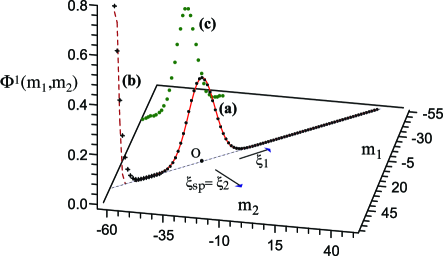
Figure 1: (Color online) A sample two-level system. The components of the exact ground state eigenvectors ($\Phi^{1}(m_{1},m_{2})$) are indicated with dots on an $(m_{1},m_{2})$ plane for (a) large and (b) small interactions. The solid and dash lines are the corresponding SHA eigenfunctions. The ground state for a different $N$ is shown by (c). The directions of the transformed coordinates, $\xi_{1}$ and $\xi_{sp}=\xi_{2}$, with their origins at the point O $\sim(j_{1}x_{o1},j_{2}x_{o2})$ are indicated for (a).

To apply the SHA to the pairing Hamiltonian (5), we define $\hat{\mathcal{H}}\Phi^{i}(\mathbf{m})=\langle{\mathbf{m}}|\hat{H}|\Phi^{i}\rangle$. Then, assuming that the low-lying eigenfunctions $\Phi^{i}(\mathbf{m})$ vary slowly with $m$, we define $k$ continuous variables $x_{p}=m_{p}/j_{p}$, and the continuous eigenfunction $\Psi^{i}(\mathbf{x})$ as before. Assuming also that the wave functions, $\Psi^{i}(\mathbf{x})$, are localized around a point $\mathbf{x}_{o}$, and that the criteria for the validity of the SHA, listed above, are satisfied, we expand the Hamiltonian $\hat{\mathcal{H}}$ up to bilinear terms in $x^{\prime}_{p}=(x_{p}-x_{op})$ and $\frac{\partial}{\partial x^{\prime}_{p}}$ to obtain

$$\hat{\mathcal{H}}\,\approx\,\, \hat{\mathcal{H}}_{\textrm{SHA}}=\sum_{p,q}^{k}\left[-{{\frac{1}{j_{p}}}\frac{\partial}{\partial x^{\prime}_{p}}A_{pq}{{\frac{1}{j_{q}}}}\frac{\partial}{\partial x^{\prime}_{q}}}+{j_{p}}x^{\prime}_{p}B_{pq}j_{q}x^{\prime}_{q}\right]$$

$$\qquad\qquad+\sum_{p}^{k}D_{p}j_{p}x^{\prime}_{p}+{E},$$ (6)

which is essentially the Hamiltonian for a coupled $k$-dimensional harmonic oscillator with the origin shifted to $x_{op}$. It contains: an inverse mass tensor $A_{pq}$, a spring constant tensor $B_{pq}$, a set of shifts $D_{p}$ and a constant $E$. Their components, defined in terms of $\kappa_{r}=(1-x_{or}^{2})$ and $T_{pq}=G_{pq}j_{p}j_{q}\sqrt{\kappa_{p}\kappa_{q}}$, are given by

$$A_{pq}=\sum_{r}T_{pr}\delta_{pq}-T_{pq},$$ (7)

$$B_{pq}=\sum_{r}T_{pr}\frac{\delta_{pq}}{{j_{p}^{2}}\kappa_{p}^{2}}-T_{pq}\frac{x_{op}x_{oq}}{{j_{p}j_{q}}\kappa_{p}\kappa_{q}},$$ (8)

$$D_{p}=2\epsilon_{p}-{G_{pp}}+\frac{2x_{op}}{j_{p}\kappa_{p}}\sum_{r}T_{pr},$$ (9)

$$E=\sum_{p}j_{p}(2\epsilon_{p}-G_{pp})(1+x_{op})-\sum_{p,q}T_{pq}.$$ (10)

The conservation of particle number in the SHA formalism is verified by showing that the SHA representation of the number operator $\hat{n}=2\sum_{p}(\hat{J}^{p}_{z}+j_{p})$ commutes with $\hat{\mathcal{H}}_{\textrm{SHA}}$. Thus, it is appropriate to make a change of variables, $j_{p}x^{\prime}_{p}\to\xi_{i}$, such that $\xi_{k}$ (denoted $\xi_{sp}$ in FIG. 1) is an $N$-dependent constant and the Hamiltonian (Eigenstate Estimation for the Bardeen-Cooper-Schrieffer (BCS) Hamiltonian) becomes that of a system of $(k\!-\!1)$ harmonic oscillators,

$$\hat{\mathcal{H}}_{\textrm{SHA}}=\sum_{i=1}^{k-1}\left(-\alpha_{i}\frac{\partial^{2}}{\partial\xi_{i}^{2}}+\beta_{i}\xi_{i}^{2}\right)+E.$$ (11)

Observe that while the dynamics of the oscillator is $(k-1)$-dimensional, the tensors $A$ and $B$ are $k$-dimensional. However, the inverse mass tensor $A$ is determined to have an eigenvector parallel to the spurious direction with zero eigenvalue; this implies that the corresponding vibrational mass is infinite, consistent with $N$ being a good quantum number in the SHA. To evaluate the quantities in eqs. (7 - 10), we need the numerical values of $x_{op}$. The point ${\bf x_{o}}$ is naturally defined as the minimum of the harmonic oscillator potential on the $(k-1)$-dimensional hyperplane (see FIG. 1). Once the pair number $N$ is selected, the numerical values of $x_{op}$ are determined by the $D_{p}$ shift functions of Eq. (9).

Having determined $x_{op}$, we can use the transformation that diagonalizes $A$ to obtain the dynamics on the hyperplane. The properties of the $(k-1)$-dimensional oscillator on the hyperplane are solved using normal-mode theory. The eigenvalues of the SHA Hamiltonian (11) are

$$\mathcal{E}_{\nu}=\sum_{i=1}^{k-1}(\nu_{i}+\tfrac{1}{2})\omega_{i}+E,$$ (12)

where $\omega_{i}=2\sqrt{{\alpha_{i}}{\beta_{i}}}$ and $\nu=\{\nu_{i}\}$ is a set of integers indicating the number of oscillator quanta in mode $i$. The corresponding set of SHA eigenfunctions are

$$\Psi_{\nu}({{\bf\xi}})=\eta\prod_{i=1}^{k-1}\big{(}2^{\nu_{i}}{\sigma_{i}}\nu_{i}!\sqrt{\pi}\big{)}^{-\frac{1}{2}}H_{\nu_{i}}({\tfrac{{\xi_{i}}}{\sigma_{i}})}e^{-\frac{1}{2}(\frac{{\xi_{i}}}{\sigma_{i}})^{2}}$$ (13)

where $H_{\nu_{i}}$ are Hermite polynomials, $\sigma_{i}=\sqrt[4]{\frac{\alpha_{i}}{\beta_{i}}}$ are the SHA widths, and $\eta$ is a normalization factor. From here, we can approximate the coefficients $\Phi^{i}(\mathbf{m})=\langle\mathbf{m}|\Phi^{i}\rangle$, and hence the eigenfunction, in the original discrete basis by evaluating $\Psi_{\nu}$ at the points ${\bf\xi}$ corresponding to $\mathbf{m}$. We refer to these approximate eigenfunctions of the Hamiltonian $\hat{H}$, as the SHA basis.

It is worth noting that the quantity $\tfrac{1}{2}(x_{op}+1)$ in the SHA can be interpreted as the mean fractional occupancy of a single-particle level $p$ in parallel with $v_{p}^{2}$ in BCS theory BCS . Similarly, the SHA shift equations for $x_{op}$ correspond to the BCS gap equations for $v_{p}^{2}$. In addition, the SHA energy $E$ is almost identical to the BCS ground state energy. It has been shown, in several model calculations, that including higher order corrections in $\frac{1}{j}$ lowers the SHA ground-state energy in the strong interaction regime below that of the BCS approximation. Thus, we obtain an insightful interpretation of the SHA treatment of the pairing model as an extension of the BCS method to a number conserving approximation which takes account of the fluctuations of the particle number in each single-particle level about its mean BCS value.

The transformed $\xi$-coordinates for a 2-level model are illustrated in FIG. 1. The SHA eigenfunction (line) corresponding to a large interaction (compared to single particle energies spacing), indicated as (a), are in good agreement with the exact components of the eigenvectors given by diagonalization. Similar accuracy is obtained for the next few higher-energy states (not shown). If greater precision is required, an even more accurate description of the low-lying eigenstates can be obtained by diagonalizing the BCS Hamiltonian in a subspace spanned by a small number of SHA basis states. For weaker interactions, as in (b), the SHA does not predict the components of the eigenvectors accurately as in (a). This is the regime in which the conditions for the validity of the SHA are not well satisfied. Nevertheless, some SHA predictions, such as $x_{op}$ and $\sigma_{i}$, remain accurate - a subtlety not yet fully understood. Thus, we can use these predictions to identify a small subset of basis states that contribute significantly to the low-lying eigenstates in the weak interaction regime and also obtain very accurate results for them by diagonalizing small Hamiltonian matrices.

To illustrate the effectiveness of the SHA, we consider a system with four degenerate single-particle energy levels. This relatively small system is selected so that exact eigenstates can be obtained by diagonalization. Based on other applications of the SHA RdeG , we expect the SHA to be even more accurate and effective in application to systems of single-particle levels of higher multiplicities.

Exact and SHA-estimated excitation energies of a sample $4$-level model with $N=28$ pairs, $j=[7,8,9,10]$ and $\epsilon=[0.5,2.3,6.1,7.3]$ are shown in FIG. 2. A simple arbitrary rule for $G$ is used: $G_{pq}=(2.0-0.1|\epsilon_{p}-\epsilon_{q}|)g$, where $g$ controls the interaction strength. Exact results are obtained by diagonalizing the $3231\times 3231$ Hamiltonian matrix.

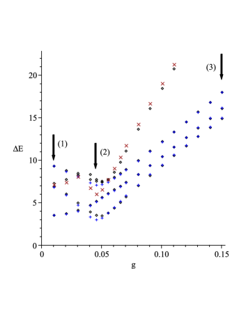
Figure 2: (Color online) The SHA predicted excitation energies for $\{n_{1},n_{2},n_{3}\}$=$\{1,0,0\},\{0,1,0\}$ and $\{0,0,1\}$ are indicated with ‘+’ and those for $\{2,0,0\}$ are indicated with ‘$\times$’. The exact lowest four excitation energies are given by ‘$\diamond$’. We mark three points of interest (1) $g=0.010$, (2) $g=0.045$ and (3) $g=0.150$. Note that the SHA excitation energies corresponding to $\{2,0,0\}$ cross-over those of $\{0,0,1\}$ at $g\sim 0.05$, indicating the system transiting from one regime to another.

For this 4-level model, the SHA oscillator in the strong interaction regime is 3-dimensional. The number of oscillator quanta in each mode is given by $\{n_{1},n_{2},n_{3}\}$. The excitation energy $\Delta\mathcal{E}_{\{n_{1},n_{2},n_{3}\}}=\mathcal{E}_{\{n_{1},n_{2},n_{3}\}}-\mathcal{E}_{\{0,0,0\}}$ for the low-lying states are shown. From the figure, we see that the SHA-predicted excitation energies (‘+’, ‘$\times$’) are in good agreement with the exact results from diagonalization (‘$\diamond$’) for a wide range of interactions. Note that while the SHA excitation energies for $g\sim 0.05$ are less accurate than for other values of $g$, the trends in how the excitation energies vary with interaction strength are still closely captured by the SHA.

Table 1: The lowest few excitation energies for (1) $g=0.010$ (2) $g=0.045$ and (2) $g=0.150$ as predicted by the SHA and diagonalizing in the most relevant subspaces (indicated by $Diag$) are shown. The ‘$Diag$’ results are given up to the digit that agrees with the corresponding exact result. All SHA predictions are given to two decimal places in (  ) with the number of oscillator quanta given in {   } in the subscript.

(1) $g=0.010$	(2) $g=0.045$	(3) $g=0.150$
$Diag_{\mathfrak{su}(2)}$ (SHA)	$Diag_{\mathfrak{su}(2)}$ (SHA)	$Diag_{\textrm{SHA}}$(SHA)
3.650313 (3.61){1,0,0}	3.60 (3.07){1,0,0}	15.03 (15.06){1,0,0}
6.9484 (6.90){0,1,0}	5.258 (5.19){0,1,0}	16.18 (16.22){0,1,0}
7.38050 (7.21){2,0,0}	7.65 (6.14){2,0,0}	18.1 (18.08){0,0,1}
9.4210 (9.38){0,0,1}	7.8 (7.20){0,0,1}	29.5 (30.12){2,0,0}
10.5531 (10.51){1,1,0}	8.37 (8.26){1,1,0}	30.7 (31.28){1,1,0}

Lastly, we show in TABLE 1 the low-lying excitation energies obtained from the SHA and by diagonalizing the BCS Hamiltonian in the space spanned by the most important basis states identified by the SHA. For points (1) and (2) in FIG. 2, the lowest $50$ and $300$ $\mathfrak{su}(2)$ basis states are used respectively. For point (3), we used the lowest 286 SHA wave functions as a basis.

The results obtained, cf. last column of TABLE 1, show the SHA to be very successful for deriving low-energy spectra of BCS Hamiltonians in the strong interaction regime in which it is most valid. They also show the SHA to be a good first-order approximation in general. As TABLE 1 indicates, accurate results can be obtained for any interaction by using the SHA to select relatively small subsets of basis states for diagonalizations.

The SHA predicts essentially the same mean level occupancies in the ground state as the BCS approximation. In addition, it gives the fluctuations in these occupancies in a manner that conserves particle number. It also conserves the $\mathfrak{su}(2)\otimes\mathfrak{su}(2)\ldots$ symmetry of the pairing Hamiltonian (defined by the values of the ${j_{p}}$ quantum numbers). The SHA gives the low-energy states of all irreps of this symmetry group. This is in contrast to the BCS approximation which is only designed to give an approximation for the ground state and quasi-particle approximations for the low-energy states of neighbouring odd-particle systems. States of maximal $\mathfrak{su}(2)\otimes\mathfrak{su}(2)\ldots$ symmetry are unbroken-pair states, whereas the broken-pair states of other irreps have unpaired particles in one or more single-particle levels. This reduces the number of states available to the paired particles so that these irreps are obtained by reducing the quasi-spin of each level $p$ by the replacement $j_{p}\to j_{p}-\tfrac{1}{2}$ for each unpaired particle in the level. The states of such irreps are handled in the same way in the SHA, except for the different values of the quasi-spins. To conclude, we note the significant possibility that the continuous variable approximation, underlying the SHA, has the potential to be applied to derive other solvable differential equations. This potential remains to be explored.

The authors wish to thank Veerle Hellemans and Trevor Welsh for their discussions. SDB is an “FWO-Vlaanderen” post-doctoral researcher and acknowledges an FWO travel grant for a “long stay abroad” at the University of Toronto and the University of Notre Dame. SYH acknowledges the funding from the National Research Foundation and the Ministry of Education (Singapore). This work was supported in part by the Natural Sciences and Engineering Research Council of Canada.

References

- (1) H. Chen, J.R. Brownstein and D.J. Rowe, Phys. Rev. C 42, 1422 (1990).
- (2) J. Bardeen, L.N. Cooper and J.R. Schrieffer, Phys. Rev. 108, 1175 (1957).
- (3) A.K. Kerman and R.D. Lawson, Phys. Rev. 124 162 (1961).
- (4) K. Dietrich, H.J. Mang, and J.H. Pradal, Phys. Rev. 135, 22 (1964).
- (5) D.J. Rowe, Nucl. Phys. A 691, 691 (2001)
- (6) J. von Delft and D.C. Ralph, Phys. Rep. 345, 61 (2001).
- (7) G.G. Dussel, S. Pittel, J. Dukelsky, and P. Sarriguren, Phys. Rev. C 76, 011302 (2007).
- (8) R.W. Richardson, Phys. Lett. B 3, 277 (1963).
- (9) M. Gaudin, J. Phys. (Paris), 37, 1087 (1976).
- (10) S. Rombouts, D. Van Neck and J. Dukelsky, Phys. Rev. C 69, 061303(R) (2004).
- (11) J. Dukelsky, C. Esebbag and P. Schuck, Phys. Rev. Lett. 87, 066403 (2001).
- (12) D.J. Rowe and H. de Guise, J. Phys. A (in press).