I Introduction

In the past several years there have been enormous progress in unraveling the structure of scattering amplitudes in gauge theory and gravity, such as generalized unitary-cut method at loop level Bern:1994zx , and Britto-Cachazo-Feng-Witten (BCFW) recursion relations at tree level, for Yang-Mills theory Britto:2004ap ; Britto:2005fq and for gravity Bedford:2005yy ; Cachazo:2005ca ; Benincasa:2007qj . A particularly important example is the structure of amplitudes in $\mathcal{N}=4$ super Yang–Mills theory (SYM), which has remarkable simplicities obscured by the usual local formulation and Feynman-diagram calculations. On the other hand, Arkani-Hamed et al. have proposed the idea that $\mathcal{N}=8$ supergravity (SUGRA) may be the quantum field theory with the simplest amplitudes ArkaniHamed:2008gz , and there is strong evidence for it: recently there have been intensive studies on both the hidden symmetries (e.g. $E_{7(7)}$ symmetry, see Kallosh:2008rr ; He:2008pb ; Brodel:2009hu ; Bossard:2010dq ), and the ultraviolet behavior of the theory (see Green:2006yu ; Bern:2007hh ; Bern:2008pv ; Bern:2009kd ; Dixon:2010gz ; Elvang:2010jv ; Drummond:2010fp ; Beisert:2010jx ; Kallosh:2010kk and references therein).

However, we do not need to go beyond the tree level to see the simplicity. As shown in ArkaniHamed:2008gz , gravity tree amplitudes satisfy non-trivial relations, or “bonus relations”, which are absent in SYM color-ordered amplitudes. These bonus relations have been applied to MHV amplitudes in Spradlin:2008bu to show the equivalence of various MHV formulae in the literature Berends:1988zp ; Nair:2005iv ; Bedford:2005yy ; Elvang:2007sg ; Mason:2008jy , especially to simplify formulae with $(n-2)!$ permutations to those with $(n-3)!$ permutations. The full strength of these relations, however, can only be demonstrated when applied to general, non-MHV amplitudes, and the purpose of the present note is to use bonus relations to simplify explicit formulae of SUGRA tree amplitudes, which are obtained by solving BCFW recursion relations. Before proceeding, let us elaborate on BCFW recursion relations and bonus relations of SUGRA amplitudes.

Supersymmetric BCFW recursion relations Brandhuber:2008pf ; ArkaniHamed:2008yf hold in both SYM and SUGRA because their amplitudes vanish when two supermomenta are taken to infinity in a complex superdirection ArkaniHamed:2008yf ; ArkaniHamed:2008gz . More specifically, under the supersymmetric BCFW shifts of momenta and $SU(\mathcal{N})$ Grassmannian variables,

$$\lambda_{\widehat{1}}(z) =\lambda_{1}+z\lambda_{n},$$ (1)

$$\widetilde{\lambda}_{\overline{n}}(z) =\widetilde{\lambda}_{n}-z\widetilde{\lambda}_{1},$$ (2)

$$\eta_{\widehat{n}}(z) =\eta_{n}-z\eta_{1},$$ (3)

SYM and SUGRA amplitudes have at least $1/z$ falloff at large $z$, thus the contour integral $\oint\frac{dz}{z}M(z)$ can be rewritten as a sum over residues without boundary contributions,

$$M_{n}=\sum_{L,R}\int d^{4\mathcal{N}}\eta M_{L}(\widehat{1},L,\{-\widehat{P}(z_{P}),\eta\})\frac{1}{P^{2}}M_{R}(\{\widehat{P}(z_{P}),\eta\},R,\overline{n}),$$ (4)

where the poles $z=z_{P}$ are determined by putting the internal momenta $\widehat{P}(z_{P})=\sum_{i\in L}P_{i}+P_{\widehat{1}}$ on shell. By solving the recursion relations, explicit formulae for up to N³MHV amplitudes, and an algorithm to calculate all tree amplitudes in SUGRA was proposed in Drummond:2009ge . The result can be written as a summation over $(n-2)!$ “ordered gravity subamplitudes” with different permutations of particles $2,\ldots,n-1$. In contrast to SYM color-ordered amplitudes, the SUGRA amplitudes actually have a faster, $1/z^{2}$, falloff and the contour integral $\oint dzM(z)$ gives the bonus relations,

$$0=\sum_{L,R}\int d^{8}\eta M_{L}(\widehat{1},L,\{-\widehat{P}(z_{P}),\eta\})\frac{z_{P}}{P^{2}}M_{R}(\{\widehat{P}(z_{P}),\eta\},R,\overline{n}).$$ (5)

Similar to the MHV case Spradlin:2008bu , we shall see that these relations can further simplify the explicit formulae for non-MHV amplitudes by reducing the $(n-2)!$-permutation sum to a new $(n-3)!$-permutation one.

Another important method that has been widely used to calculate gravity tree amplitudes are Kawai-Lewellen-Tye (KLT) relations, first derived in string theory Kawai:1985xq which express (super)gravity tree amplitudes as sums of products of two copies of (super)Yang–Mills amplitudes in the field-theory limit. Recently KLT relations have been proved in gravity BjerrumBohr:2010ta ; BjerrumBohr:2010zb and in SUGRA Feng:2010br using BCFW recursion relations, without resorting to string theory. While the well-known KLT relations have a form of $(n-3)!$ permutations Bern:1998sv (see also BjerrumBohr:2010zb ), in the proof it is natural to use the newly proposed $(n-2)!$ form suitable for BCFW recursion relations BjerrumBohr:2010ta , and a direct link between these two forms has been derived in Feng:2010hd . In a related approach, the so-called square relations between gravity and Yang-Mills amplitudes, which can be viewed as a reformulation of KLT relations, have been proposed and proved in Bern:2008qj . These relations also possess a freedom of going from $(n-2)!$-permutation form to the simpler $(n-3)!$ form, which, similar to the freedom in KLT relations, reflects the Bern-Carrasco-Johansson (BCJ) relations between Yang-Mills amplitudes Bern:2008qj . For SUGRA amplitudes, the advantage of having solved BCFW relations to some extent will enable us to go beyond this implicit freedom following from BCJ relations, and show the simplification of gravity amplitudes directly in their explicit forms.

The note is organized as following. In section 2 we briefly review tree amplitudes in SUGRA and their bonus relations, especially the simplification of MHV amplitudes when using these relations. Then we apply these relations to some examples beyond MHV amplitudes, including the NMHV and N²MHV amplitudes, and prove these simplified formulae in section 3. The generalization to all tree-level SUGRA amplitudes are presented in section 4.

II A brief review of tree amplitudes in SUGRA and bonus relations

II.1 Tree Amplitudes in SUGRA from BCFW Recursion Relations

By solving Eq. (4), all color-ordered SYM tree amplitudes have been obtained and can be written schematically as Drummond:2008cr ,

$$A_{n}(1,...,n)=A^{\rm{MHV}}(1,\ldots,n)\sum_{\alpha}R_{\alpha}(1,\ldots,n),$$ (6)

where

$$A^{\rm{MHV}}(1,\ldots,n)=\frac{\delta^{8}(\sum_{i}\lambda_{i}\eta_{i})}{\langle 12\rangle\langle 23\rangle\cdots\langle n1\rangle}$$ (7)

is the MHV superamplitudes, and $R_{\alpha}$ are the so-called dual superconformal invariants, which, for N^kMHV amplitudes, are products of $k$ basic invariants of the form,

$$R_{n;a_{1}b_{1};a_{2}b_{2};\ldots;a_{r}b_{r};ab}=\frac{\langle aa-1\rangle\langle bb-1\rangle\ \delta^{(4)}(\langle\xi|x_{b_{r}a}x_{ab}|\theta_{bb_{r}}\rangle+\langle\xi|x_{b_{r}b}x_{ba}|\theta_{ab_{r}}\rangle)}{x_{ab}^{2}\langle\xi|x_{b_{r}a}x_{ab}|b\rangle\langle\xi|x_{b_{r}a}x_{ab}|b-1\rangle\langle\xi|x_{b_{r}b}x_{ba}|a\rangle\langle\xi|x_{b_{r}b}x_{ba}|a-1\rangle}\,,$$ (8)

where the chiral spinor $\xi$ is given by

$$\langle\xi|=\langle n|x_{na_{1}}x_{a_{1}b_{1}}x_{b_{1}a_{2}}x_{a_{2}b_{2}}\ldots x_{a_{r}b_{r}}\,,$$ (9)

and dual (super)coordinates are defined as

$$x_{ij} =p_{i}+p_{i+1}+\cdots+p_{j-1}\,,$$ (10)

$$\theta_{ij} =\lambda_{i}\eta_{i}+\cdots+\lambda_{j-1}\eta_{j-1}\,.$$ (11)

\psfrag{one}[cc][cc]{$1$}\psfrag{a1b1}[cc][cc]{$a_{1}b_{1}$}\psfrag{a2b2}[cc][cc]{$a_{2}b_{2}$}\psfrag{a3b3}[cc][cc]{$a_{3}b_{3}$}\psfrag{b1a1a2b2}[cc][cc]{$a_{1}b_{1};a_{2}b_{2}$}\psfrag{b2a2a3b3}[cc][cc]{$a_{2}b_{2};a_{3}b_{3}$}\psfrag{b1a1a3b3}[cc][cc]{$a_{1}b_{1};a_{3}b_{3}$}\psfrag{b1a1b2a2a3b3}[cc][cc]{$a_{1}b_{1};a_{2}b_{2};a_{3}b_{3}$}\psfrag{two}[cc][cc]{$2$}\psfrag{n1}[cc][cc]{$n$}\psfrag{a1p}[cc][cc]{$a_{1}$}\psfrag{a2p}[cc][cc]{$a_{2}$}\psfrag{b1}[cc][cc]{$b_{1}$}\psfrag{b2}[cc][cc]{$b_{2}$}\epsfbox{tree.eps}

Figure 1: An rooted tree diagram for tree-level SYM amplitudes. The figure is the same as the tree diagram presented in Drummond:2009ge .

\psfrag{uvs}[cc][cc]{$u_{1}v_{1};\ldots u_{r}v_{r};a_{p-1}b_{p-1}$}\psfrag{uvab}[cc][cc]{$u_{1}v_{1};\ldots u_{r}v_{r};a_{p-1}b_{p-1};a_{p}b_{p}$}\psfrag{uvnext}[cc][cc]{$u_{1}v_{1};\ldots u_{r}v_{r};a_{p}b_{p}$}\psfrag{ab}[cc][cc]{$a_{p}b_{p}$}\psfrag{up}[cc][cc]{$a_{p-1}$}\psfrag{bp1}[cc][cc]{$b_{p-1}$}\psfrag{bvr}[cc][cc]{$v_{r}$}\psfrag{bv1}[cc][cc]{$v_{1}$}\psfrag{n1}[cc][cc]{$n$}\psfrag{dots}[cc][cc]{$\ldots$}\epsfbox{genericterm.eps}

Figure 2: The rule for going from line $p-1$ to line $p$ (for $p>1$) in Fig. 1. For every vertex in line $p-1$ of the form given at the top of the diagram, there are $r+2$ vertices in the lower line (line $p$). The labels in these vertices start with $u_{1}v_{1};\ldots u_{r}v_{r};a_{p-1}b_{p-1};a_{p}b_{p}$ and they get sequentially shorter, with each step to the right removing the pair of labels adjacent to the last pair $a_{p},b_{p}$ until only the last pair is left. The summation limits between each line are also derived from the labels of the vertex above. The left superscripts which appear on the associated $R$-invariants start with $u_{1}v_{1}\ldots u_{r}v_{r}b_{p-1}a_{p-1}$ for the left-most vertex. The next vertex to the right has the superscript $u_{1}v_{1}\ldots u_{r}v_{r}a_{p-1}b_{p-1}$, i.e. the same as the first but with the final pair in alphabetical order. The next vertex has the superscript $u_{1}v_{1}\dots u_{r}v_{r}$ and thereafter the pairs are sequentially deleted from the right.

There is only one invariant $R=1$ for MHV case, while we have a sum of $R_{n;a_{1}b_{1}}$ with $1<a_{1}<b_{1}<n$ for NMHV case. Furthermore, for N²MHV case we have $R_{n;a_{1}b_{1}}R^{b_{1}a_{1}}_{n;a_{1}b_{1},a_{2}b_{2}}$ with $1<a_{1}<a_{2}<b_{2}\leq b_{1}<n$ and $R_{n;a_{1}b_{1}}R^{a_{1}b_{1}}_{n;a_{2}b_{2}}$ with $1<a_{1}<b_{1}\leq a_{2}<b_{2}<n$, where superscripts denote boundary modifications of these invariants Drummond:2008cr .

Generally the summation variables $\alpha$, and boundary modifications, can be represented by a rooted tree diagram Drummond:2008cr ; Drummond:2009ge (see Fig. 1 and Fig. 2). For N^kMHV amplitudes, there are $C_{k}=\frac{(2k)!}{k!(k+1)!}$ (Catalan number) types of terms labeled by $\alpha$’s corresponding to a path from the root to the $k$-th level in Fig. 1, and each type can be written as a list of $k$ pairs of labels with a particular order between them, $\alpha\equiv\{n;a_{1},b_{1};\ldots;a_{k},b_{k}\}$. Not only does the summation over $\alpha$ include all types of terms, but it also sums over all possible $1<a_{i},b_{i}<n$ in the corresponding order.

In Drummond:2009ge , solving Eq. (4) for SUGRA is simplified by using ordered gravity subamplitude $M(1,\ldots,n)$, which satisfy the ordered BCFW recursion relations similar to Yang-Mills theory,

$$M(1,\ldots,n)\equiv\sum_{i=3}^{n-1}\int\frac{d^{8}\eta}{P^{2}}M(\widehat{1},2,\ldots,i-1,\widehat{P})M(-\widehat{P},i,\ldots,n-1,\overline{n})\,,$$ (12)

and the sum of $(n-2)!$ permutations of ordered gravity subamplitudes gives the full amplitude,

$$\mathcal{M}_{n}=\sum_{\mathcal{P}(2,3,\ldots,n-1)}M(1,\ldots,n).$$ (13)

A solution for $M(1,\ldots,n)$ is obtained in Drummond:2009ge ,

$$M(1,...,n)=[A^{\rm{MHV}}(1,\ldots,n)]^{2}\sum_{\alpha}G_{\alpha}R^{2}_{\alpha}(1,\ldots,n),$$ (14)

where the invariants $R_{\alpha}$ are exactly the same as those in SYM (including boundary modifications), namely products of basic invariants (8), with the same set of summation variables $\alpha$ as given in Fig. 1 and Fig. 2, and the ‘dressing factors’, $G_{\alpha}$, are independent of the Grassmannian variables $\eta_{i}$, and they break dual conformal invariance of the SYM solution. These factors have been calculated explicitly for up to N³MHV amplitudes, for example MHV case,

$$G^{\rm MHV}(1,\ldots,n)=x_{13}^{2}\prod_{s=2}^{n-3}\frac{\langle s|x_{s,s+2}x_{s+2,n}|n\rangle}{\langle sn\rangle}\,,$$ (15)

and there is an algorithm to calculate them in general cases, but we do not need their expressions in this note. In addition, tree-level amplitudes of $n$-graviton scattering can be obtained from SUGRA superamplitudes (13), by choosing fermionic coordinates $\eta=0$ for positive-helicity gravitons, and integrating over $d^{8}\eta$ for negative-helicity ones. Details of the solution can be found in Drummond:2009ge .

Therefore, SUGRA tree amplitude can be written as a summation of $(n-2)!$ ordered gravity subamplitudes, and each of them has a structure similar to SYM ordered amplitude. In the following we shall use bonus relations to reduce this form to a simpler, $(n-3)!$ form, and first we recall the simplest MHV case.

II.2 Applying Bonus Relations to MHV Amplitudes

Applying bonus relation to MHV SUGRA tree-level amplitudes was well understood in Spradlin:2008bu . From Eq. (15), we have the MHV amplitudes as a summation of $(n-2)!$ terms,

$$\mathcal{M}_{n}^{\rm{MHV}}=G^{\rm MHV}(1,\ldots n)[A^{\rm{MHV}}(1,\ldots,n)]^{2}+\mathcal{P}(2,3,\ldots,n-1).$$ (16)

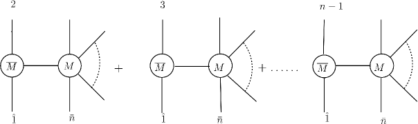
Figure 3: All factorizations contributing to (17) for the MHV amplitude.

From Fig. 3, we see that there are $(n-2)$ BCFW factorizations and thus the formula can be expressed as,

$$\mathcal{M}_{n}^{\rm{MHV}}=M_{2}+M_{3}+\ldots+M_{n-1},$$ (17)

where each $M_{i}$ is a BCFW term from $\overline{\rm{MHV}}(\widehat{1},i,\widehat{P}(z_{i}))\times\rm{MHV}_{n-1}$ with $z_{i}=-\frac{\langle 1i\rangle}{\langle ni\rangle}$. Now since the amplitude has $1/z^{2}$ fall off, we have a bonus relation which is simple in the MHV case,

$$0=z_{2}M_{2}+z_{3}M_{3}+\ldots+z_{n-1}M_{n-1}.$$ (18)

Using this relation, we can express the last diagram $M_{n-1}$ in terms of the other $n-3$ diagrams, and a simple manipulation gives us a $(n-3)!$-term formula,

$$\mathcal{M}_{n}^{\rm MHV} =B^{\rm MHV}G^{\rm MHV}(1,2,\dots,n)[A^{\rm MHV}(1,2,\dots,n)]^{2}$$ (19)

$$+\mathcal{P}(2,3,\dots,n-2).$$

where we have defined the MHV bonus coefficient $B^{\rm MHV}=\frac{\langle 1~{}n\rangle\langle n-1~{}n-2\rangle}{\langle 1~{}n-1\rangle\langle n~{}n-2\rangle}$. Beyond MHV, we have many more types of BCFW diagrams with complicated structures and the application of bonus relations becomes trickier. In the next section, we shall work out the NMHV and N²MHV cases, and then move on to general amplitudes in section 4.

III Applying Bonus Relations to Non-MHV Gravity Tree Amplitudes

III.1 General Strategy

Before moving on to examples, we first explain the general strategy for applying bonus relations to non-MHV gravity tree amplitudes. For a N^kMHV amplitude, inhomogeneous contributions of the form N^pMHV $\times$ N^qMHV are needed $(p+q+1=k)$. Naively one would like to use “bonus-simplified” lower-point amplitudes for both $M_{L}$ and $M_{R}$ in Eq. (4), but this is not compatible with the fact that we can only delete one diagram (not two) by applying the bonus relations (5), if we want to preserve the structure of ordered BCFW recursion relations.

To keep the advantages of the ordered BCFW recursion relations, which are crucial to solve for all tree-level amplitudes, instead we shall apply bonus relations selectively. The idea is illustrated in Fig. 4. Similar to the MHV case, we shall delete Fig. 4(d) by using bonus relations (5). To compute the inhomogeneous parts of the amplitudes, we shall use the bonus-simplified amplitude only on one side of a BCFW diagram, namely the lower-point amplitude with the leg $(n-1)$ in it, as indicated in Fig. 4(a) and Fig. 4(b).

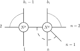
(a) Inhomogeneous diagram type I

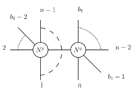
(b) Inhomogeneous diagram type II

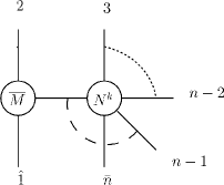
(c) Homogeneous diagram

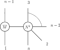
(d) Diagram deleted by bonus relations

Figure 4: Different types of diagrams for a general N^kMHV amplitude, where $k=p+q+1$. We use a dashed line $----$ connecting three legs to denote a bonus-simplified lower-point amplitude, in which these three legs are kept fixed. For lower-point amplitudes without dashed lines, we use the usual $(n-2)$! form.

In this way, the amplitude splits into two types, one type coming from the diagrams of the form as in Fig. 4(a), which has the leg $(n-1)$ adjacent to the leg $n$ and will be called the normal, or type I contributions, and the other one coming from those having the form as in Fig. 4(b), which has the leg $(n-1)$ exchanged with another leg $(b_{1}-1)$, and will be called the exchanged, or type II contributions,

$$\mathcal{M}_{n}=\big{[}A_{n}^{\rm MHV}\big{]}^{2}\big{(}\sum_{\alpha}B^{(1,m_{1})}_{\alpha}G_{\alpha}R^{2}_{\alpha}+\sum_{\beta}B^{(2,m_{2})}_{\beta}[G_{\beta}R^{2}_{\beta}(b_{1}-1\leftrightarrow n-1)]\big{)}+\mathcal{P}(2,3,\dots,n-2),$$ (20)

where $(b_{1}-1\leftrightarrow n-1)$ denotes the exchanges of momenta $(p_{b_{1}-1}\leftrightarrow p_{n-1})$ as well as the fermionic coordinates $(\eta_{b_{1}-1}\leftrightarrow\eta_{n-1})$, and we have used square bracket to indicate that the exchanges act only on the expression inside the bracket. The superscript $(i,m_{i})$ in $B^{(i,m_{i})}_{\alpha}$ is used to show the type of this contribution, which will become clear in the examples.

Thus we have seen that, by using bonus relations, any amplitude can be written as a summation of $(n-3)!$ permutations with the coefficients $B^{(i,m_{i})}_{\alpha}$, which will be called bonus coefficients. In this section, we shall calculate all bonus coefficients for NMHV and N²MHV cases, and generalize the pattern observed in these examples to general N^kMHV amplitudes in the next section. Once bonus coefficients are calculated, we obtain explicitly all simplified SUGRA tree amplitudes.

III.2 NMHV Amplitudes

Here we use bonus relations to simplify the $(n-2)!$ form of NMHV amplitudes. First we shall state the general simplified form of NMHV amplitudes, and then prove it by induction. To be concise, we abbreviate the combinations

$$\{n;a_{1}b_{1}\}\equiv G_{n;a_{1}b_{1}}\big{[}R_{n;a_{1}b_{1}}A^{{\rm MHV}}(1,2,\dots,n)\big{]}^{2}$$ (21)

and similar notations will be used in the following sections.

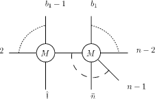
(a) Inhomogeneous diagram type I

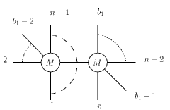
(b) Inhomogeneous diagram type II

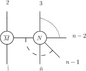
(c) Homogeneous diagram

Figure 5: Diagrams for NMHV amplitudes.

As mentioned above generally, we delete the contributions corresponding to Fig. 4(d) by using the bonus relation (5). It is straightforward to compute the inhomogeneous contributions from the two MHV $\times$ MHV diagrams, Fig. 5(a) and Fig. 5(b). Firstly, let us consider the contribution from Fig. 5(a), which corresponds to terms with $a_{1}=2$, and we have

$$M_{1}=B^{(1)}_{n;2b_{1}}\{n;2b_{1}\},~{}~{}~{}{\rm with}~{}~{}4\leq b_{1}\leq n-1,$$ (22)

where $B^{(1)}_{n;2b_{1}}$ are the special cases of the general bonus coefficients $B^{(1)}_{n;a_{1}b_{1}}$. We have used the superscript $(1)$ to indicate that this is the contribution coming from type-I diagram, and similar notations will be used below.

When $b_{1}\neq n-1$, the bonus coefficients are given by,

$$B^{(1)}_{n;a_{1}b_{1}}=B^{\rm MHV}\frac{\langle n-1|x_{b_{1}a_{1}}x_{b_{1}n}|n\rangle}{\langle n-1|x_{b_{1}a_{1}}x_{a_{1}n}|n\rangle}.$$ (23)

Here we note that we can get the above coefficients from the previous ones, namely the bonus coefficients of MHV amplitude, multiplied by the factor $\frac{\langle n-1|x_{b_{1}a_{1}}x_{b_{1}n}|n\rangle}{\langle n-1|x_{b_{1}a_{1}}x_{a_{1}n}|n\rangle}.$ It is a general feature of this type of coefficients, for N^kMHV case they are given by N^k-1MHV coefficients multiplied by the same factor, as we shall see explicitly again in the N²MHV case.

However when $b_{1}=n-1$, no bonus relation can be used for the right-hand-side 3-point MHV amplitude in Fig. 5(a), and we find

$$B^{(1)}_{n;a_{1}n-1}=\frac{\langle 1~{}n\rangle}{\langle 1~{}n-1\rangle}\frac{\langle n-1|x_{n-1a_{1}}|n-1]}{\langle n|x_{na_{1}}|n-1]}.$$ (24)

For the exchanged diagrams, Fig. 5(b), the contribution can be similarly obtained

$$M_{2} =B^{(2)}_{n;2b_{1}}[\{n;2a_{1}\}(b_{1}-1\leftrightarrow n-1)],~{}~{}~{}{\rm with}~{}~{}4\leq b_{1}\leq n-1,$$ (25)

where the bonus coefficients $B^{(2)}_{n;a_{1}b_{1}}$ are given by

$$B^{(2)}_{n;a_{1}b_{1}} =\frac{\langle 1~{}n\rangle}{\langle 1~{}n-1\rangle}\frac{\langle n-1~{}b_{1}-2\rangle(x^{\prime}_{a_{1}b_{1}})^{2}}{\langle n|x_{na_{1}}x^{\prime}_{a_{1}b_{1}}|b_{1}-2\rangle},$$ (26)

and we have defined $x^{\prime}_{a_{i}b_{i}}$ as,

$$x^{\prime}_{a_{i}b_{i}} \equiv x_{a_{i}b_{i}-1}+x_{n-1n}$$ (27)

$$= x_{a_{i}b_{i}}(p_{b_{i}-1}\leftrightarrow p_{n-1}).$$

All the above calculations do not include the boundary case $a_{1}=n-3,b_{1}=n-1$, which needs special treatment. This boundary case is special because it recursively reduces to the special 5-point NMHV ($\overline{\rm{MHV}}$) amplitude. It does not have the diagram of the type $\overline{{\rm MHV}}_{3}\times$ NMHV, and one has to treat it separately. We apply the bonus relations to this case in the following way: we use Eq. (5) to delete the contribution from Fig. 6(a), and compute Fig. 6(b), and we find

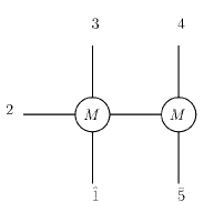
(a) $5$-point diagram deleted by bonus relation

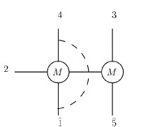
(b) $5$-point diagram

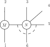
(c) $6$-point diagram calculating the boundary contribution

Figure 6: Diagrams for $5$-point NMHV amplitude and the boundary term of $6$-point NMHV amplitude. Fig. 6(a) and Fig. 6(b) are used to calculate the bonus-simplified, $5$-point, right-hand-side amplitude of Fig. 6(c).

$$\mathcal{M}_{5}=-\frac{[24][34][51]}{[23][45][41]}\big{[}\{5;24\}(3\leftrightarrow 4)\big{]}+\mathcal{P}(2,3).$$ (28)

By plugging the above 5-point result in Fig. 6(c), we get the boundary term of the 6-point NMHV amplitude

$$M^{\rm(boundary)}_{6}=\frac{\langle 16\rangle\langle 25\rangle[35][45]x_{36}^{2}}{\langle 15\rangle[34]\langle 2|1+6|5]\langle 6|1+2|5]}\big{[}\{6;35\}(4\leftrightarrow 5)\big{]}.$$ (29)

A generic form for the boundary term of the $n$-point NMHV amplitudes can be obtained as a straightforward generalization of (28) and (29),

$$M^{(\rm{boundary})}_{n}=B^{({\rm boundary})}_{n;n-3~{}n-1}\big{[}\{n;n-3~{}n-1\}(n-2\leftrightarrow n-1)\big{]},$$ (30)

where $B^{(\rm boundary)}_{n;n-3~{}n-1}$ is given by,

$$B^{({\rm boundary})}_{n;n-3~{}n-1}=\frac{\langle 1n\rangle\langle n-4~{}n-1\rangle[n-3~{}n-1][n-2~{}n-1]x^{2}_{n-3n}}{\langle 1~{}n-1\rangle[n-3~{}n-2]\langle n-4|x_{n-3~{}n-1}|n-1]\langle n|x_{n-1~{}n-3}|n-1]}.$$ (31)

Putting everything together, we obtain the general formula for NMHV amplitude and as promised, the amplitude indeed can be written as a sum of $(n-3)!$ permutations

$$\mathcal{M}_{n}^{\rm{NMHV}} = \sum^{n-4}_{a_{1}=2}\sum^{n-1}_{b_{1}=a_{1}+2}\left(B^{(1)}_{n;a_{1}b_{1}}\{n;a_{1}b_{1}\}+B^{(2)}_{n;a_{1}b_{1}}[\{n;a_{1}b_{1}\}(b_{1}-1\leftrightarrow n-1)]\right)+M^{(\rm{boundary})}_{n}$$ (33)

$$+\mathcal{P}(2,3,\dots,n-2).$$

III.2.1 Proof by Induction

Here we shall give an inductive proof for the simplified NMHV formula. For $a_{1}=2$, as we explained above, the formula follows directly from Fig. 5(a) and Fig. 5(b). Therefore we shall focus on the cases when $a_{1}\geq 3$, which correspond to the homogeneous contributions from Fig. 5(c). We shall prove that the formula satisfies the BCFW recursion relations.

First note that we have deleted one diagram of the form $M^{\rm{MHV}}_{L}(\hat{1},n-1,\hat{P})\times M^{\rm{MHV}}_{R}$ by using bonus relations, this results in a multiplicative prefactor for the overall amplitude, which is given by,

$$(1-\frac{z_{2}}{z_{n-1}})=\frac{\langle 1n\rangle\langle n-1~{}2\rangle}{\langle n2\rangle\langle 1n-1\rangle}.$$ (34)

Let us consider the bonus coefficient $B^{(1)}_{n;a_{1}b_{1}}$, other coefficients $B^{(2)}_{n;a_{1}b_{1}}$ and $B^{({\rm boundary})}_{n;n-3~{}n-1}$ can be treated similarly. By plugging formula (23) into the $(n-1)$-point amplitude $M(-{\hat{P}},3,4,\ldots,n-1,{\bar{n}})$ in Fig. 5(c), it is straightforward to check that the second piece of $B^{(1)}_{n;a_{1}b_{1}}$, $\frac{\langle n-1|x_{b_{1}a_{1}}x_{b_{1}n}|n\rangle}{\langle n-1|x_{b_{1}a_{1}}x_{a_{1}n}|n\rangle}$, is transformed back to itself under the recursion relations.

For the first piece $B^{\rm MHV}=\frac{\langle n-1~{}n-2\rangle\langle 1~{}n\rangle}{\langle n~{}n-2\rangle\langle 1~{}n-1\rangle}$ of $B^{(1)}_{n;a_{1}b_{1}}$, which is the MHV bonus coefficient, the proof is essentially the same as in the MHV case. Taking into account the factor in (34) coming from bonus relations, we have

$$\frac{\langle n-1~{}n-2\rangle\langle{\hat{p}}~{}n\rangle}{\langle n~{}n-2\rangle\langle{\hat{p}}~{}n-1\rangle}\times\frac{\langle 1~{}n\rangle\langle n-1~{}2\rangle}{\langle 1~{}n-1\rangle\langle n~{}2\rangle}=\frac{\langle n-1~{}n-2\rangle\langle 1~{}n\rangle}{\langle n~{}n-2\rangle\langle 1~{}n-1\rangle}.$$ (35)

Thus the contribution with $B^{(1)}_{n;a_{1}b_{1}}$ indeed satisfies the recursion relations.

A final remark is in order. We have used in the proof that $\{n;a_{1}b_{1}\}$ satisfy the ordered BCFW recursion relations by themselves.

III.3 N²MHV amplitudes

In this subsection we consider N²MHV amplitudes as one more example to show the general features of bonus-simplified gravity amplitudes. Similar to NMHV case, let us denote the ordered gravity solutions in the following way

$$H^{(1)}_{n;a_{1}b_{1},a_{2}b_{2}}\big{[}R_{n;a_{1}b_{1}}R^{b_{1}a_{1}}_{n;a_{1}b_{1},a_{2}b_{2}}A^{{\rm MHV}}(1,2,\dots,n)\big{]}^{2} \equiv \{n;a_{1}b_{1},a_{2}b_{2}\}_{1},$$

$$H^{(2)}_{n;a_{1}b_{1},a_{2}b_{2}}\big{[}R_{n;a_{1}b_{1}}R^{a_{1}b_{1}}_{n;a_{2}b_{2}}A^{{\rm MHV}}(1,2,\dots,n)\big{]}^{2} \equiv \{n;a_{1}b_{1},a_{2}b_{2}\}_{2}.$$

There are four relevant types of diagrams (and a boundary case) which contribute to the general N²MHV amplitudes. The general structure of N²MHV is given in Fig. 7 and the corresponding contributions from each of the four diagrams can be calculated separately.

First we consider the contributions from the diagrams in Fig. 7(b), which are of the form MHV$\times$ NMHV. We use bonus-simplified amplitude for the right-hand-side NMHV amplitude and we obtain,

$$M_{{\rm I}} = \sum_{2\leq a_{1},b_{1}\leq n-1}\sum_{b_{1}\leq a_{2},b_{2}<n}\big{(}B_{n;a_{1}b_{1};a_{2}b_{2}}^{(1,1)}\{n;a_{1}b_{1};a_{2}b_{2}\}_{2}$$ (36)

$$+~{}B_{n;a_{1}b_{1};a_{2}b_{2}}^{(1,2)}[\{n;a_{1}b_{1};a_{2}b_{2}\}_{2}(b_{2}-1\leftrightarrow n-1)]\big{)}$$

$$+\sum_{2\leq a_{1},b_{1}\leq n-1}B_{n;a_{1}b_{1};n-3n-1}^{(1,{\rm boundary})}[\{n;a_{1}b_{1};n-3n-1\}_{2}(n-2\leftrightarrow n-1)],$$

where in the first sum $a_{2}\leq n-4$ because of the range of summation of the first term in Eq. (33). Here the bonus coefficients are given by

$$B_{n;a_{1}b_{1};a_{2}b_{2}}^{(1,1)} = \frac{\langle 1n\rangle\langle n-1~{}n-2\rangle\langle n-1|x_{a_{2}b_{2}}x_{b_{2}n}|n\rangle}{\langle 1n-1\rangle\langle n~{}n-2\rangle\langle n-1|x_{a_{2}b_{2}}x_{a_{2}n}|n\rangle}\frac{\langle n-1|x_{a_{1}b_{1}}x_{b_{1}n}|n\rangle}{\langle n-1|x_{a_{1}b_{1}}x_{a_{1}n}|n\rangle}\quad$$

$$B_{n;a_{1}b_{1};a_{2}b_{2}}^{(1,1)} = \frac{\langle 1n\rangle\langle n-1|x_{n-1a_{2}}|n-1]}{\langle 1n-1\rangle\langle n|x_{na_{2}}|n-1]}\frac{\langle n-1|x_{a_{1}b_{1}}x_{b_{1}n}|n\rangle}{\langle n-1|x_{a_{1}b_{1}}x_{a_{1}n}|n\rangle}\quad(b_{2}=n-1)$$

$$B_{n;a_{1}b_{1};a_{2}b_{2}}^{(1,2)} = \frac{\langle 1n\rangle\langle n-1~{}b_{2}-2\rangle(x^{\prime}_{a_{2}b_{2}})^{2}}{\langle 1n-1\rangle\langle n|x_{na_{2}}x^{\prime}_{a_{2}b_{2}}|b_{2}-2\rangle}\frac{\langle n-1|x_{a_{1}b_{1}}x_{b_{1}n}|n\rangle}{\langle n-1|x_{a_{1}b_{1}}x_{a_{1}n}|n\rangle}$$

$$B_{n;a_{1}b_{1};n-3n-1}^{(1,{\rm boundary})} = B^{({\rm boundary})}_{n;n-3~{}n-1}\frac{\langle n-1|x_{a_{1}b_{1}}x_{b_{1}n}|n\rangle}{\langle n-1|x_{a_{1}b_{1}}x_{a_{1}n}|n\rangle},$$ (37)

where the last term $B_{n;a_{1}b_{1};n-3n-1}^{(1,{\rm boundary})}$ comes from Eq. (31). Again the superscripts are used to show the types of the contributions. For instance, in the superscript $(1,1)$ of $B_{n;a_{1}b_{1};a_{2}b_{2}}^{(1,1)}$, the first $``1"$ means that it is the type-I contribution, while the second $``1"$ implies that it is a descendant from the NMHV case. A generalization to the N^kMHV case will be $B_{n;a_{1}b_{1};\dots;a_{k}b_{k}}^{(m)}$, where $m$ is a string composed of three kinds of labels, “$1$” “$2$” and “boundary”.

As we have mentioned in the NMHV case, and we want to stress it here again that the bonus coefficients of Fig. 7(b) are simply given as the previous ones, namely the coefficients of NMHV amplitudes, with replacements $(a_{1}\rightarrow a_{2},b_{1}\rightarrow b_{2})$ and multiplied by the same factor $\frac{\langle n-1|x_{a_{1}b_{1}}x_{b_{1}n}|n\rangle}{\langle n-1|x_{a_{1}b_{1}}x_{a_{1}n}|n\rangle}$.

Next, we calculate the contributions from the diagrams in Fig. 7(c) which are of the form NMHV$\times$ MHV and we get

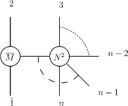
(a) Homogeneous diagram

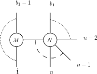
(b) Inhomogeneous diagram type I

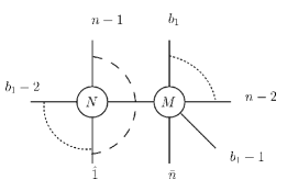
(c) Inhomogeneous diagram type II

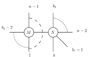
(d) Inhomogeneous diagram type II

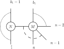
(e) Inhomogeneous diagram type I

Figure 7: Diagrams for N²MHV amplitudes.

$$\begin{aligned} M_{{\rm II}}=&\sum_{2\leq a_{1},b_{1}\leq n-1}\sum_{a_{1}\leq a_{2},b_{2}<b_{1}}\big{(}B_{n;a_{1}b_{1};a_{2}b_{2}}^{(2,1)}\{n;a_{1}b_{1};a_{2}b_{2}\}_{1}(n-1\leftrightarrow b_{1}-1)\\ &+B_{n;a_{1}b_{1};a_{2}b_{2}}^{(2,2)}[\{n;a_{1}b_{1};a_{2}b_{2}\}_{1}(b_{2}-1\leftrightarrow b_{1}-1)]\big{)}\\ &+\sum_{2\leq a_{1}\leq n-3}B_{n;a_{1}n-1;n-4n-2}^{(2,{\rm boundary})}[\{n;a_{1}n-1;n-3n-1\}_{1}(n-2\leftrightarrow n-1)].\end{aligned}$$ (38)

In the above sum we do not include the boundary case $(a_{1},b_{1},a_{2},b_{2})=(n-4,n-1,n-4,n-2)$, which we shall study separately. The coefficients are given by

$$\begin{aligned} B_{n;a_{1}b_{1};a_{2}b_{2}}^{(2,1)}&=\frac{\langle 1n\rangle\langle n-1~{}b_{1}-2\rangle\langle n-1|x_{b_{2}a_{2}}x^{\prime}_{b_{2}b_{1}}x^{\prime}_{a_{1}b_{1}}x_{a_{1}n}|n\rangle(x^{\prime}_{a_{1}b_{1}})^{2}}{\langle 1n-1\rangle\langle b_{1}-2|x^{\prime}_{a_{1}b_{1}}x_{a_{1}n}|n\rangle\langle n-1|x_{b_{2}a_{2}}x^{\prime}_{a_{2}b_{1}}x^{\prime}_{a_{1}b_{1}}x_{a_{1}n}|n\rangle}\\ B_{n;a_{1}b_{1};a_{2}b_{2}}^{(2,1)}&=\frac{\langle 1n\rangle\langle n-1|x_{n-1a_{2}}|n-1](x^{\prime}_{a_{1}b_{1}})^{2}}{\langle 1n-1\rangle\langle n|x_{na_{1}}x^{\prime}_{a_{1}b_{1}}x^{\prime}_{b_{1}a_{2}}|n-1]}\quad(b_{2}=n-2)\\ B_{n;a_{1}b_{1};a_{2}b_{2}}^{(2,2)}&=\frac{\langle 1n\rangle\langle n-1~{}b_{2}-2\rangle(x^{\prime}_{a_{2}b_{2}})^{2}(x^{\prime}_{a_{1}b_{1}})^{2}}{\langle 1n-1\rangle\langle n|x_{na_{1}}x^{\prime}_{a_{1}b_{1}}x^{\prime}_{b_{1}a_{2}}x^{\prime}_{a_{2}b_{2}}|b_{2}-2\rangle}\\ B_{n;a_{1}b_{1};n-4n-2}^{(2,{\rm boundary})}&=\frac{\langle 1n\rangle\langle b_{1}-4~{}n-1\rangle[b_{1}-3~{}n-1][b_{1}-2~{}n-1](x^{\prime}_{b_{1}-3b_{1}})^{2}(x^{\prime}_{a_{1}b_{1}})^{2}}{\langle 1~{}n-1\rangle[b_{1}-3~{}b_{1}-2]\langle b_{1}-4|x_{b_{1}-4~{}b_{1}-1}|n-1]\langle n|x_{na_{1}}x^{\prime}_{a_{1}b_{1}}x_{b_{1}-1b_{1}-3}|n-1]}.\end{aligned}$$ (39)

By comparing the results with those of NMHV, now we are ready to see the patterns. For this type of diagrams Fig. 7(c), the bonus coefficients can be obtained from the results of NMHV by doing the following replacements on the indices of region momenta $x$’s: $n\rightarrow b_{1},a_{1}\rightarrow a_{2},b_{1}\rightarrow b_{2}$, and $x\rightarrow x^{\prime}$ when $x$ has the index $n$ with it. Furthermore one should apply the changes on $\langle n|$ and $\langle n-i|$, which correspondingly read $\langle n|\rightarrow\langle n|x_{na_{1}}x^{\prime}_{a_{1}b_{1}}$, and $\langle n-i|({\rm or}~{}[n-i|)\rightarrow\langle b_{1}-i|({\rm or}~{}[b_{1}-i|)$ for $i>1$. Finally we multiply the obtained answers by a factor $(x^{\prime}_{a_{1}b_{1}})^{2}$.

The bonus coefficients of the contributions from other diagrams are actually the same as those of the NMHV case. For the sake of completeness, let us write down these contributions: for the contribution from Fig. 7(d), we have

$$M_{{\rm III}}=\sum_{2\leq a_{1},b_{1}\leq n-1}\sum_{b_{1}\leq a_{2},b_{2}<n}B_{n;a_{1}b_{1};a_{2}b_{2}}^{(2)}[\{n;a_{1}b_{1};a_{2}b_{2}\}_{2}(b_{1}-1\leftrightarrow n-1)],$$ (40)

where the bonus coefficients $B_{n;a_{1}b_{1};a_{2}b_{2}}^{(2)}$ are given by Eq. (26); for the other contribution coming from Fig. 7(e), we get

$$M_{{\rm IV}}=\sum_{2\leq a_{1},b_{1}\leq n-1}\sum_{a_{1}\leq a_{2},b_{2}<b_{1}}B_{n;a_{1}b_{1};a_{2}b_{2}}^{(1)}\{n;a_{1}b_{1};a_{2}b_{2}\}_{1},$$ (41)

and similarly the coefficients are given by Eq. (23) and Eq. (24).

Again as in the case of Eq. (38), this formula does not include the boundary case, $\{n;a_{1}b_{1};a_{2}b_{2}\}_{1}=\{n;n-4n-1;n-4n-2\}_{1}$, which should be considered separately, as we shall do below.

Similar to 5-point NMHV amplitude, the 6-point N²MHV amplitude is special which only receives contributions from diagrams of NMHV $\times$ MHV type and we must treat it separately. We can delete Fig. 8(a) by bonus relations, and the contribution from Fig. 8(b) gives,

$$\mathcal{M}_{6}=-\frac{[16][25][45]}{[15][24][56]}[\{6;25,24\}_{1}(3\leftrightarrow 5)]+\mathcal{P}(2,3,4).$$ (42)

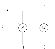
(a) $6$-point diagram deleted by bonus relations

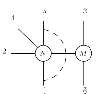
(b) $6$-point diagram

Figure 8: Diagrams for $6$-point N²MHV amplitude.

As the NMHV case (30), 6-point N²MHV amplitude (42) can also be similarly generalized, and we obtain the boundary term of the full $n$-point N²MHV amplitudes,

$$M^{({\rm boundary})}_{n} = B^{(\rm boundary)}_{n;n-4~{}n-1;n-4~{}n-2}[\{n;n-4~{}n-1;n-4~{}n-2\}_{1}(n-3\leftrightarrow n-1)],$$ (43)

where the bonus coefficients are given as

$$B^{(\rm boundary)}_{n;n-4~{}n-1;n-4~{}n-2}=\frac{\langle 1n\rangle\langle n-5~{}n-1\rangle[n-4~{}n-1][n-2~{}n-1]x_{n-4n}^{2}}{\langle 1n-1\rangle[n-4~{}n-2]\langle n-5|x_{n-4~{}n-1}|n-1]\langle n|x_{n-1~{}n-4}|n-1]}.$$ (44)

Therefore we have calculated all the contributions for N²MHV amplitudes and as in the NMHV case, it can also be written as a sum of $(n-3)!$ permutations,

$$\mathcal{M}_{n}^{{\rm N}^{2}{\rm MHV}}=M_{{\rm I}}+M_{{\rm II}}+M_{{\rm III}}+M_{{\rm IV}}+M^{({\rm boundary})}_{n}+\mathcal{P}(2,3,\ldots,n-2).$$ (45)

The result can be proved very similarly by induction as in the NMHV case.

IV Generalization to all gravity tree amplitudes

Now we have all the ingredients for generalizing our results and stating the patterns for all tree-level gravity amplitudes. Our way of using bonus relations gives the simplified tree-level N^kMHV superamplitude as a sum of $(n-3)!$ permutations, and each of them contains normal and exchanged contributions,

$$\mathcal{M}^{{\rm N}^{k}\rm{MHV}}_{n}=\big{[}A_{n}^{\rm MHV}\big{]}^{2}\big{(}\sum_{\alpha}B^{(1,m_{1})}_{\alpha}G_{\alpha}R^{2}_{\alpha}+\sum_{\beta}B^{(2,m_{2})}_{\beta}[G_{\beta}R^{2}_{\beta}(b_{1}-1\leftrightarrow n-1)]\big{)}+\mathcal{P}(2,3,\ldots,n-2).$$ (46)

For both the contributions we have $k$ types of terms from $k$ BCFW channels, namely N^pMHV $\times$ N^qMHV, for $p+q+1=k$ with $0\leq p,q<k$ by reducing the homogeneous term recursively. As we have stressed repeatedly, to respect the ordered structure, we have only used bonus relations on one lower-point amplitude, namely the right-hand-side N^qMHV for normal contribution, and the left-hand-side N^pMHV for exchanged contribution.

Before presenting all the bonus coefficients for general tree amplitudes, we pause to show by induction that bonus relations roughly reduce the number of terms from $(n-2)!$ in the original solution to $(k+1)(n-3)!$ in the simplified one. To get the previous counting we note that in the N^pMHV$\times$ N^qMHV channel of the normal contribution, by applying bonus relations to the N^qMHV lower-point amplitude we can reduce the number of terms from $(n-2)!/k$ to $(q+1)(n-3)!/k$. Taking into account all channels gives us $(1+2+\ldots+k)(n-3)!/k$ terms, with the same number from the exchanged contribution, thus the simplified form has only $(k+1)(n-3)!$ terms. By parity, one only needs N^kMHV amplitudes with $n>2k+2$ legs and thus the bonus relations can be used to delete at least half of the terms in tree amplitudes. The simplification becomes more significant when $n\gg k$.

Now we generalize the pattern found in the NMHV and N²MHV cases to write down all the bonus coefficients for general tree amplitudes. As we have learned from the examples, once the bonus coefficients of N^k-1MHV amplitudes are calculated, then for the N^kMHV amplitudes, one only needs to compute two types of new contributions for N^kMHV amplitudes, namely the normal contribution from ${\rm MHV}\times{\rm N}^{k-1}{\rm MHV}$ channel ($q=k-1$) and the exchanged contribution from ${\rm N}^{k-1}{\rm MHV}\times{\rm MHV}$ channel ($p=k-1$) (see Fig. 9). All other bonus coefficients $B^{(m)}_{\alpha}$ of N^pMHV $\times$ N^qMHV with $q<k-1$ and $p<k-1$, are the same as those computed previously, namely the results from N^k-1MHV amplitudes. Since the summation variables of N^kMHV amplitude can be obtained by adding a pair of new labels $a_{k},b_{k}$ to the previous one, $\alpha^{\prime}$, $\alpha=\{\alpha^{\prime};a_{k},b_{k}\}$, the result can be written as

$$B^{(m)}_{\alpha} = B^{(m)}_{\alpha^{\prime}},$$ (47)

for both normal contributions with $q<k-1$ and exchanged ones with $p<k-1$.

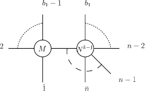
(a) ${\rm MHV}\times{\rm N}^{k-1}{\rm MHV}$

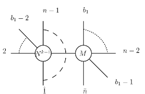
(b) ${\rm N}^{k-1}{\rm MHV}\times{\rm MHV}$

Figure 9: Two relevant diagrams for computing new bonus coefficients for $n$-point N^kMHV amplitude. The rest of the bonus coefficients can be obtained recursively from the N^k-1MHV case.

Thus we only need to calculate two new contributions from Fig. 9(a) and Fig. 9(b). It is straightforward to confirm that all the observations we have made for the cases of NMHV and N²MHV can be directly generalized to all tree-level amplitudes. First we shall state the rules and then justify them. Firstly, just like Eq. (23) and Eq. (III.3) for NMHV and N²MHV cases, the bonus coefficients of Fig. 9(a), $B^{(1,m_{1})}_{\alpha}$, can be similarly obtained by the replacements on the indices of the region momenta $x$’s, $a_{i}\rightarrow a_{i+1},b_{i}\rightarrow b_{i+1}$, for $B^{(m_{1})}_{\alpha^{\prime}}$ of N^k-1MHV amplitudes, then multiplying with a simple common factor of the form $\frac{\langle n-1|x_{a_{1}b_{1}}x_{b_{1}n}|n\rangle}{\langle n-1|x_{a_{1}b_{1}}x_{a_{1}n}|n\rangle}$, which are the same for all tree-level amplitudes,

$$B^{(1,m_{1})}_{\alpha}=\frac{\langle n-1|x_{a_{1}b_{1}}x_{b_{1}n}|n\rangle}{\langle n-1|x_{a_{1}b_{1}}x_{a_{1}n}|n\rangle}B^{(m_{1})}_{\alpha^{\prime}}(a_{i}\rightarrow a_{i+1},b_{i}\rightarrow b_{i+1}).$$ (48)

Secondly, the bonus coefficients for the new exchanged contributions Fig. 9(b), $B^{(2,m_{2})}_{\beta}$, can be obtained by taking $B^{(m_{2})}_{\beta^{\prime}}$ of N^k-1MHV amplitudes, and performing the following replacements on the indices of region momenta $x$’s, namely $n\rightarrow b_{1},a_{i}\rightarrow a_{i+1},b_{i}\rightarrow b_{i+1}$, and $x\rightarrow x^{\prime}$ when $x$ has index $n$ with it. And for the spinors, we have $\langle n|\rightarrow\langle n|x_{na_{1}}x^{\prime}_{a_{1}b_{1}}$ as well as $|n-i\rangle({\rm or}~{}|n-i])\rightarrow|b_{1}-i\rangle({\rm or}~{}|b_{1}-i])$ for $i>1$. In addition, the obtained answers are further multiplied by a factor $(x^{\prime}_{a_{1}b_{1}})^{2}$,

$$B^{(2,m_{2})}_{\beta} = (x^{\prime}_{a_{1}b_{1}})^{2}B^{(m_{2})}_{\beta^{\prime}},$$ (49)

where the arguments of $B^{(m_{2})}_{\beta^{\prime}}$ should be changed under the rules we described above.

All these rules can be understood in a simple way. For the rules of the normal contributions, the common factor is obtained in the following way,

$$(1-\frac{z_{i}}{z_{n-1}})\frac{\langle n1\rangle}{\langle n-11\rangle}\rightarrow(1-\frac{z_{i}}{z_{n-1}})\frac{\langle n\widehat{P}\rangle}{\langle n-1\widehat{P}\rangle}\rightarrow\frac{\langle n-1|x_{a_{1}b_{1}}x_{b_{1}n}|n\rangle}{\langle n-1|x_{a_{1}b_{1}}x_{a_{1}n}|n\rangle},$$ (50)

where $(1-\frac{z_{i}}{z_{n-1}})$ comes from the fact that we delete one diagram using bonus relations, and $\frac{\langle n1\rangle}{\langle n-11\rangle}$ is a factor that always appears in every bonus coefficient.

While for the rules of the exchanged contributions, we find that the factor $(x^{\prime}_{a_{1}b_{1}})^{2}$ appears because

$$\langle n1\rangle\rightarrow\langle\widehat{P}\widehat{1}\rangle\rightarrow[\widehat{P}\widehat{1}]\langle\widehat{P}\widehat{1}\rangle\rightarrow(x^{\prime}_{a_{1}b_{1}})^{2},$$ (51)

and $\langle n|$ changes in the following way under the recursion relations,

$$\langle n|\rightarrow\langle\widehat{P}|\rightarrow\langle n1\rangle[1\widehat{P}]\langle\widehat{P}|\rightarrow\langle n|x_{na_{1}}x^{\prime}_{a_{1}b_{1}}.$$ (52)

Besides, the transformation rule of $x_{n\gamma_{i}}$ follows as

$$x_{n\gamma_{i}}\rightarrow x_{\widehat{P}\gamma_{i+1}}\rightarrow x^{\prime}_{b_{1}\gamma_{i+1}},$$ (53)

where $\gamma$ can be $a$ or $b$ and we have used the fact that $p_{\widehat{P}}=p_{b_{1}}+\dots+p_{n-2}+p_{b_{1}-1}+p_{\widehat{n}}.$ So in this way, we have a complete understanding of the rules we have proposed.

Finally, as shown in the examples a boundary contribution has to be considered separately because the special case $(k+4)$-point N^kMHV amplitude only has diagrams of N^k-1MHV $\times$ MHV type. For this special contribution, it is straightforward to obtain a general form,

$$M^{({\rm boundary})}_{n} = B^{(\rm{boundary})}_{\beta_{0}}\big{[}\big{(}A_{n}^{\rm MHV}\big{)}^{2}G_{\beta_{0}}R^{2}_{\beta_{0}}(n-k-1\leftrightarrow n-1)\big{]},$$ (54)

where $\beta_{0}=\{n;n-k-2~{}n-1;n-k-2~{}n-2;\ldots;n-k-2~{}n-k\}$, and the coefficients can be written as

$$B^{(\rm{boundary})}_{\beta_{0}}=\frac{\langle 1n\rangle\langle n-k-3~{}n-1\rangle[n-k-2~{}n-1][n-k~{}n-1]x^{2}_{n-k-2~{}n}}{\langle 1n-1\rangle[n-k-2~{}n-2]\langle n-k-3|x_{n-k-3~{}n-1}|n-1]\langle n|x_{n-1~{}n-k-2}|n-1]}.$$ (55)

Therefore, we have found a set of explicit rules to write down all the bonus coefficients for all tree amplitude in $\mathcal{N}=8$ supergravity.

V Conclusion and outlook

In this note, we simplified tree-level amplitudes in $\mathcal{N}=8$ SUGRA, from the BCFW form with a sum of $(n-2)!$ permutations to a new form as a sum of $(n-3)!$ permutations. This is achieved by using the bonus relations, which are relations between tree amplitudes in theories without color ordering. In contrast to the MHV case, a naive use of the bonus relations ruins the structure of the non-MHV ordered tree-level solution, thus we proposed an improved application of the relations, which respects the ordered structure. The key point here is to apply the bonus relations to only one of two lower-point amplitudes in any BCFW diagram, which indeed brings SUGRA amplitudes to a simplified form having a $(n-3)!$-permutation sum with some bonus coefficients. To illustrate the method, we have explicitly calculated simplified amplitudes for the NMHV and N²MHV cases. We have also argued that the pattern generalizes to N^kMHV cases, and presented a simple way for writing down the bonus coefficients of all amplitudes, thus one can recursively obtain the simplified form for general SUGRA tree amplitudes.

The simplification is based on an explicit solution from BCFW recursion relations of SUGRA tree amplitudes of Drummond:2009ge , which is in spirit similar to but in details different from KLT relations. From a computational point of view, any gravity amplitude obtained from $(n-3)!$ (or the newly proposed $(n-2)!$) form of KLT relations is a sum of $(n-3)!^{2}$ (or $(n-2)!^{2}$) terms; at least in the special case of $\mathcal{N}=8$ SUGRA, an explicit solution with only $(n-2)!$ terms was found in Drummond:2009ge , which is a significant simplification. Furthermore, in this note we have used the bonus relations to reduce it to a sum with only $(k+1)(n-3)!$ terms. Further simplifications of gravity tree amplitudes are certainly worth investigating.

Apart from the computational advantages, the simplification is also conceptually interesting. The relations between gravity and gauge theories have been reexamined from various perspectives recently Bern:2008qj ; BjerrumBohr:2010ta ; BjerrumBohr:2010zb (see also Nastase:2010xa ). A common feature, of these “gravity”$=$“gauge theory”² methods, is the freedom of rewriting $(n-2)!$ forms of gravity tree amplitudes as $(n-3)!$ forms, essentially by using BCJ relations on the gauge theory side. Our result confirms this freedom at an explicit level by directly using it to simplify SUGRA amplitudes, which also suggests that bonus relations may be regarded as explicit gravity relations induced by Yang-Mills BCJ relations. It may be fruitful to understand the exact connections between our method, general forms of KLT relations, and the square relations. In particular, it would be nice to go beyond SUGRA and see if similar simplifications occur generally, given that both BCFW recursion relations and bonus relations are valid in more general gravity theories.

Bonus relations and simplifications we obtained at tree level can also have implications for loop amplitudes. Through the generalized unitarity-cut method, our new form of tree amplitudes can be used in calculations of loop amplitudes. In addition, the square relations have been conjectured to hold at loop level Bern:2010ue , thus we may expect similar simplifications directly for the SUGRA loop amplitudes.

- (1) Z. Bern, L. J. Dixon, D. C. Dunbar and D. A. Kosower, Nucl. Phys. B 425, 217 (1994) [arXiv:hep-ph/9403226]. Z. Bern, L. J. Dixon, D. C. Dunbar and D. A. Kosower, Nucl. Phys. B 435, 59 (1995) [arXiv:hep-ph/9409265].
- (2) R. Britto, F. Cachazo and B. Feng, Nucl. Phys. B 715, 499 (2005) [arXiv:hep-th/0412308].
- (3) R. Britto, F. Cachazo, B. Feng and E. Witten, Phys. Rev. Lett. 94, 181602 (2005) [arXiv:hep-th/0501052].
- (4) J. Bedford, A. Brandhuber, B. J. Spence and G. Travaglini, Nucl. Phys. B 721, 98 (2005) [arXiv:hep-th/0502146].
- (5) F. Cachazo and P. Svrcek, arXiv:hep-th/0502160.
- (6) P. Benincasa, C. Boucher-Veronneau and F. Cachazo, JHEP 0711, 057 (2007) [arXiv:hep-th/0702032].
- (7) N. Arkani-Hamed, F. Cachazo and J. Kaplan, JHEP 1009, 016 (2010) [arXiv:0808.1446 [hep-th]].
- (8) R. Kallosh and T. Kugo, JHEP 0901, 072 (2009) [arXiv:0811.3414 [hep-th]].
- (9) S. He and H. Zhu, JHEP 1007, 025 (2010) [arXiv:0812.4533 [hep-th]].
- (10) J. Broedel and L. J. Dixon, JHEP 1005, 003 (2010) [arXiv:0911.5704 [hep-th]].
- (11) G. Bossard, C. Hillmann and H. Nicolai, arXiv:1007.5472 [hep-th].
- (12) M. B. Green, J. G. Russo and P. Vanhove, Phys. Rev. Lett. 98, 131602 (2007) [arXiv:hep-th/0611273].
- (13) Z. Bern, J. J. Carrasco, L. J. Dixon, H. Johansson, D. A. Kosower and R. Roiban, Phys. Rev. Lett. 98, 161303 (2007) [arXiv:hep-th/0702112].
- (14) Z. Bern, J. J. M. Carrasco, L. J. Dixon, H. Johansson and R. Roiban, Phys. Rev. D 78, 105019 (2008) [arXiv:0808.4112 [hep-th]].
- (15) Z. Bern, J. J. Carrasco, L. J. Dixon, H. Johansson and R. Roiban, Phys. Rev. Lett. 103, 081301 (2009) [arXiv:0905.2326 [hep-th]].
- (16) L. J. Dixon, arXiv:1005.2703 [hep-th].
- (17) H. Elvang, D. Z. Freedman and M. Kiermaier, arXiv:1003.5018 [hep-th].
- (18) J. M. Drummond, P. J. Heslop and P. S. Howe, arXiv:1008.4939 [hep-th].
- (19) N. Beisert, H. Elvang, D. Z. Freedman, M. Kiermaier, A. Morales and S. Stieberger, Phys. Lett. B 694, 265 (2010) [arXiv:1009.1643 [hep-th]].
- (20) R. Kallosh, arXiv:1009.1135 [hep-th].
- (21) M. Spradlin, A. Volovich and C. Wen, Phys. Lett. B 674, 69 (2009) [arXiv:0812.4767 [hep-th]].
- (22) F. A. Berends, W. T. Giele and H. Kuijf, Phys. Lett. B 211, 91 (1988).
- (23) V. P. Nair, Phys. Rev. D 71, 121701 (2005) [arXiv:hep-th/0501143].
- (24) H. Elvang and D. Z. Freedman, JHEP 0805, 096 (2008) [arXiv:0710.1270 [hep-th]].
- (25) L. Mason and D. Skinner, arXiv:0808.3907 [hep-th].
- (26) A. Brandhuber, P. Heslop and G. Travaglini, Phys. Rev. D 78, 125005 (2008) [arXiv:0807.4097 [hep-th]].
- (27) N. Arkani-Hamed and J. Kaplan, JHEP 0804, 076 (2008) [arXiv:0801.2385 [hep-th]].
- (28) J. M. Drummond, M. Spradlin, A. Volovich and C. Wen, Phys. Rev. D 79, 105018 (2009) [arXiv:0901.2363 [hep-th]].
- (29) H. Kawai, D. C. Lewellen and S. H. H. Tye, Nucl. Phys. B 269, 1 (1986).
- (30) N. E. J. Bjerrum-Bohr, P. H. Damgaard, B. Feng and T. Sondergaard, arXiv:1005.4367 [hep-th].
- (31) N. E. J. Bjerrum-Bohr, P. H. Damgaard, B. Feng and T. Sondergaard, Phys. Lett. B 691, 268 (2010) [arXiv:1006.3214 [hep-th]]. N. E. J. Bjerrum-Bohr, P. H. Damgaard, B. Feng and T. Sondergaard, JHEP 1009, 067 (2010) [arXiv:1007.3111 [hep-th]].
- (32) B. Feng and S. He, JHEP 1009, 043 (2010) [arXiv:1007.0055 [hep-th]].
- (33) Z. Bern, L. J. Dixon, M. Perelstein and J. S. Rozowsky, Nucl. Phys. B 546, 423 (1999) [arXiv:hep-th/9811140].
- (34) B. Feng, S. He, R. Huang and Y. Jia, JHEP 1010, 109 (2010) [arXiv:1008.1626 [hep-th]].
- (35) Z. Bern, J. J. M. Carrasco and H. Johansson, Phys. Rev. D 78, 085011 (2008) [arXiv:0805.3993 [hep-ph]]. Z. Bern, T. Dennen, Y. t. Huang and M. Kiermaier, Phys. Rev. D 82, 065003 (2010) [arXiv:1004.0693 [hep-th]].
- (36) J. M. Drummond and J. M. Henn, JHEP 0904, 018 (2009) [arXiv:0808.2475].
- (37) H. Nastase and H. J. Schnitzer, arXiv:1011.2487 [hep-th].
- (38) Z. Bern, J. J. M. Carrasco and H. Johansson, Phys. Rev. Lett. 105, 061602 (2010) [arXiv:1004.0476 [hep-th]].